Classification of Liver Diseases Based on Ultrasound Image Texture Features


1
Graduate Institute of Automation and Control, National Taiwan University of Science and Technology, Taipei City 10607, Taiwan
2
Division of Gastroenterology and Hepatology, Department of Internal Medicine, Taipei Medical University Hospital, Taipei City 11031, Taiwan
3
Division of Gastroenterology and Hepatology, Department of Internal Medicine, School of Medicine, College of Medicine, Taipei Medical University, Taipei City 11031, Taiwan
4
Department of Occupational Medicine, Taipei Medical University Hospital, Taipei City 11031, Taiwan
5
Department of Family Medicine, School of Medicine, College of Medicine, Taipei Medical University, Taipei City 11031, Taiwan
6
School of Public Health, College of Public Health and Nutrition, Taipei Medical University, Taipei City 11031, Taiwan
*
Author to whom correspondence should be addressed.
Appl. Sci. 2019, 9(2), 342; https://0-doi-org.brum.beds.ac.uk/10.3390/app9020342
Submission received: 10 December 2018
/
Revised: 7 January 2019
/
Accepted: 8 January 2019
/
Published: 19 January 2019
(This article belongs to the Special Issue Selected Papers from IEEE ICKII 2018)
Abstract
:This paper discusses using computer-aided diagnosis (CAD) to distinguish between hepatocellular carcinoma (HCC), i.e., the most common type of primary liver malignancy and a leading cause of death in people with cirrhosis worldwide, and liver abscess based on ultrasound image texture features and a support vector machine (SVM) classifier. Among 79 cases of liver diseases including 44 cases of liver cancer and 35 cases of liver abscess, this research extracts 96 features including 52 features of the gray-level co-occurrence matrix (GLCM) and 44 features of the gray-level run-length matrix (GLRLM) from the regions of interest (ROIs) in ultrasound images. Three feature selection models—(i) sequential forward selection (SFS), (ii) sequential backward selection (SBS), and (iii) F-score—are adopted to distinguish the two liver diseases. Finally, the developed system can classify liver cancer and liver abscess by SVM with an accuracy of 88.875%. The proposed methods for CAD can provide diagnostic assistance while distinguishing these two types of liver lesions.
Keywords:
classification; F-score; gray-level co-occurrence matrix (GLCM); gray-level run-length matrix (GLRLM); hepatocellular carcinoma (HCC); liver cancer; liver abscess; image texture; sequential backward selection (SBS); sequential forward selection (SFS); support vector machine (SVM); ultrasound images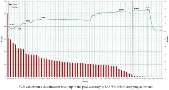
1. Introduction
Liver diseases are among the most life-threatening diseases worldwide. Among the different kinds of liver lesions, liver cancer has a high incidence rate and high mortality rate in the countries of East Asia, Southeast Asia, sub-Saharan Africa, and Melanesia [1]. Liver abscess is less common than liver cancer. However, if it is not detected in time and treated in the proper manner, it may cause many serious infectious complications, even death. Liver biopsy is often used to evaluate liver diseases. It permits doctors to examine a liver and provides helpful information to make high-accuracy predictions. Along with those undeniable benefits, it may cause pain, infection or other injuries that hinder later treatments.
To reduce the unnecessary number of biopsy cases, other noninvasive methods for diagnosis have been applied widely, especially imaging techniques such as ultrasound (US) (e.g., see [2,3,4,5,6,7,8,9]), computed tomography (CT) (e.g., see [4,10,11,12,13,14,15]) or magnetic resonance imaging (MRI) (e.g., see [2,3,12,16]). Among those methods, ultrasound imaging, with unique advances advantages such as no radiation, low cost, easy operation, and noninvasiveness, is widely used to visualize the liver for clinical diagnoses. Therefore, it could provide visual information for doctors to identify the state of disease. Nevertheless, the diagnoses are significantly affected by the quality of ultrasound images as well as the doctors’ knowledge and experience. For inexperienced clinicians, it may be not easy to distinguish between liver cancers and liver abscess.
To overcome the obstacles mentioned above, it would be helpful to develop a computer-aided diagnosis (CAD) system (e.g., see [15,17,18]). By using image processing and machine learning techniques, a well-built system could help clinicians effectively and objectively distinguish liver diseases. Multiple scientists have studied the classification of liver diseases based on ultrasound images. For example, Nicholas et al. first exploited textural features to discriminate between liver and spleen of normal humans [19]. Richard and Keen utilized Laws’ five-by-five feature mask and then applied a probabilistic relaxation algorithm to the segmentation [20]. Many textural features were used by Pavlopoulos et al. for quantitative characterization of ultrasonic images [21]. Bleck et al. used the random field model to distinguish the four states of the liver [22]. The models proposed by Kadah et al. and Gebbinck et al. combined neural networks and discriminant analysis to separate the different liver disease [23,24]. Pavlopoulos et al. improved their model by using fuzzy neural networks to process the features [25]. Horng et al. evaluated the efficiency of the textural spectrum, the fractal dimension, the textural feature coding method, and the gray-level co-occurrence matrix in distinguishing cirrhosis, normal samples, and hepatitis [26]. Yang et al. developed an algorithm for classifying cirrhotic and noncirrhotic liver with the spleen-referenced approach [27].
As mentioned above, analyzing and classifying images presenting organ lesions to differentiate benign and malignant lesions is a goal shared by many researchers. There are still few clinically relevant studies on ultrasound imaging to explore the CAD-based differential diagnosis of hepatocellular carcinoma and liver abscess, even though many studies have analyzed the characteristics of hepatocellular carcinoma (HCC) (e.g., see [28,29]) or liver abscess (e.g., see [30,31]). Recently, many methods have been proposed to extract the features from ultrasound images. For instance, first- and second-order statistics have been used (e.g., see [32]). Other approaches based on wavelet transform (e.g., see [33]), Gabor filter (e.g., see [34]), monogenic decomposition (e.g., see [35]), or fractal analysis (e.g., see [36]) were also proposed.
A CAD system to distinguish between liver cancer and liver abscess has not been discussed. The main objective of this paper is to develop a reliable CAD system to distinguish between hepatocellular carcinoma (HCC), i.e., the most common type of primary liver malignancy and a leading cause of death in people with cirrhosis worldwide, and liver abscess based on the support vector machine (SVM) method [37,38,39,40,41] and ultrasound images of textural features. To date, there is no algorithm that is best in machine learning. A good classifier depends on the data. Some algorithms work with certain data or applications better than others. The major advantage of SVM is the need for fewer parameters to make it operational with high accuracy rates, and various features can be extracted. However, the textural feature applied the most is the gray-level co-occurrence matrix (GLCM) (e.g., see [42,43,44,45,46]). GLCM feature extraction, proposed by Haralick [42] in 1973 to analyze an image as a texture, belongs to the second-order statistics. GLCM means a tabulation of the frequencies or how often a combination of pixel brightness values in an image occurs. In this paper, the other method we used to analyze the ROIs is the gray-level run-length matrix (GLRLM) (e.g., see [47,48,49,50,51]). It was first proposed by Galloway in 1975 with five features [47]. GLRLM is a matrix including the texture features that can be extracted for texture analysis. In 1990, Chu et al. [48] suggested two new features to extract gray-level information in the matrix before Dasarathy and Holder [49] offered another four features following the idea of a joint statistical measure of gray level and run length. Tang [50] provided a good summary of some features achieved by the GLRLM. In this paper, we compared the results from the popular features of the GLCM and the gray-level run-length matrix (GLRLM).
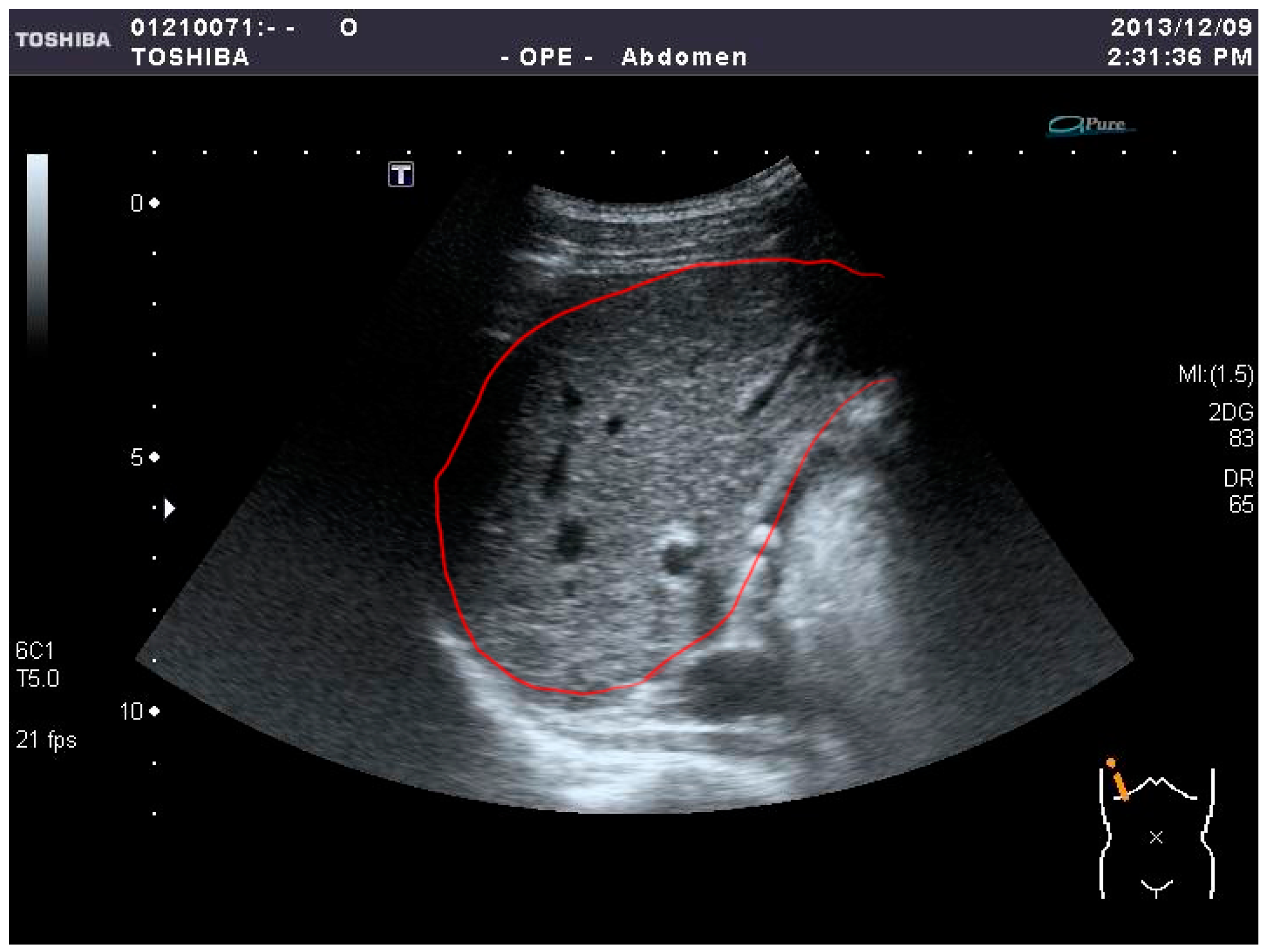
In this paper, three feature selection models—(i) sequential forward selection (SFS) [52,53], (ii) sequential backward selection (SBS) [53,54], and (iii) F-score [55]—are adopted to distinguish the two liver diseases. Marill and Green introduced a feature selection technique using the divergence distance as the criterion function and the SBS method as the search algorithm [52,53]. Whitney discussed its ‘bottom-up’ counterpart, known as SFS [53,54]. In this research, a large number of features are included, comprising 96 features from each sample. If all of them are used to train a classifier, it not only takes too much time but also cannot easily achieve high accuracy. To reduce the processing time and improve the accuracy, it is necessary to search for the important features from the feature set. Then, the crucial features of the samples are used to train and test by SVM. We took several steps to achieve this goal. First, in the ultrasound images, the liver lesions are marked by experienced physicians and the regions of interest (ROIs) are circled inside a red boundary, as illustrated in Figure 1, meaning that part of the liver lesion is located inside the red boundary of the whole-liver image. Second, all features are extracted from the collected ROIs. Third, several feature selection processes are carried out to optimize the feature set. Finally, the optimal feature sets are used to train and test by SVM.
2. Feature Extraction
Feature extraction is one of the most important stages in pattern recognition. It collects the input data for a classifier and thus can directly affect the performance of a CAD system. For example, with the same number of features, a better feature set could more exactly describe the special characteristics of each kind of liver disease such that it can improve the diagnostic result. As mentioned in Section 1, textural analysis of US images is a very useful tool for liver diagnosis, and two of the most effective methods are GLCM and GLRLM. In this research, we extract 96 features including 52 features of GLCM and 44 features of GLRLM, for analysis.
2.1. Materials
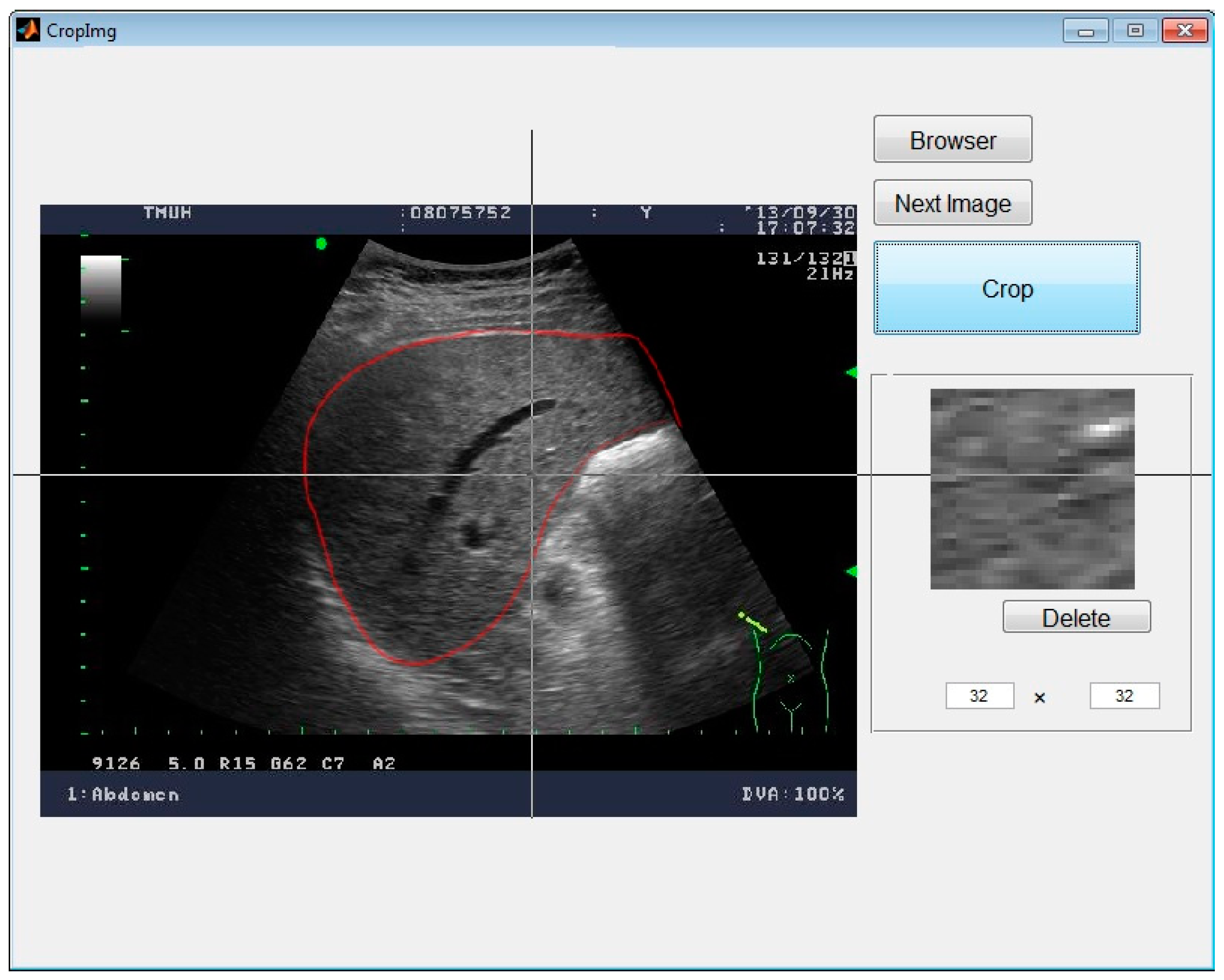
In medical imaging, the protocol of Digital Imaging and Communications in Medicine (DICOM) [12] is the standard for the communication and management of medical imaging information; therefore, DICOM files are typically used. In this research, for the convenience of image analysis, the original US images, supported by the Medical University Hospital in Taipei, were stored and then converted into 256-grayscale BMP files by MATLAB for more convenient processing. The images were from 79 cases of liver diseases including 44 cases of HCC and 35 cases of liver abscess. First, the original images were marked by experienced clinicians and verified in clinical reality. Then, the 32 × 32-pixel ROIs were selected inside the marked boundaries, as presented in Figure 1. In Figure 2, the 32 × 32-pixel ROIs were sampled from the marked image. All samples were collected from the liver disease images for later procedures, as shown in Figure 3. In this research, we sampled 400 ROIs of each kind of disease for training and testing.
2.2. GLCM and Haralick Features
In this step, ROIs are analyzed by GLCM, the most popular second-order statistical feature, proposed by Haralick [42] in 1973. Haralick feature extraction is completed in two steps. In the first step, the co-occurrence matrix is calculated and in the second, the texture features, which are very useful in a variety of imaging applications, particularly in biomedical imaging, are computed based on the co-occurrence matrix.
2.2.1. GLCM
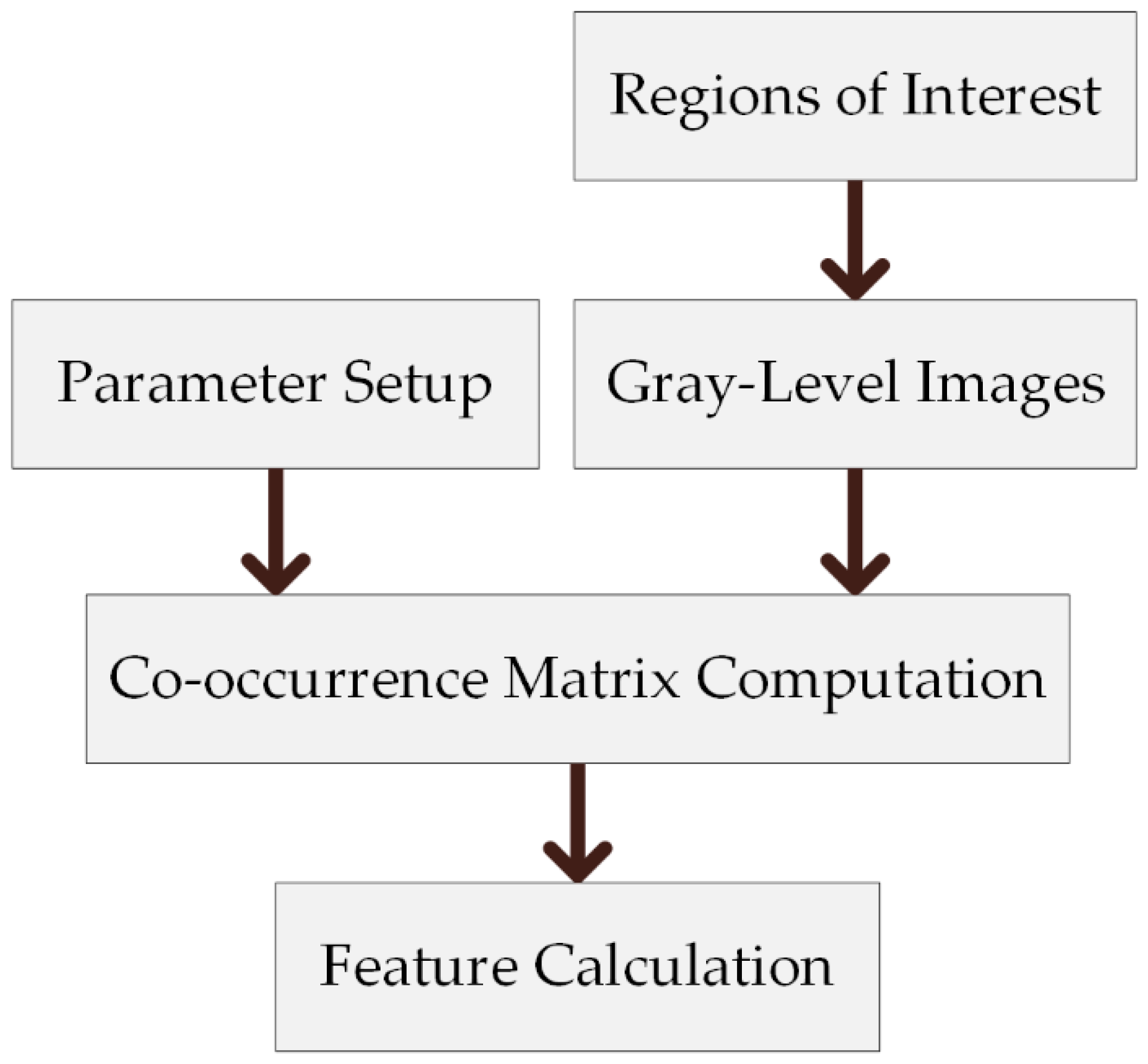
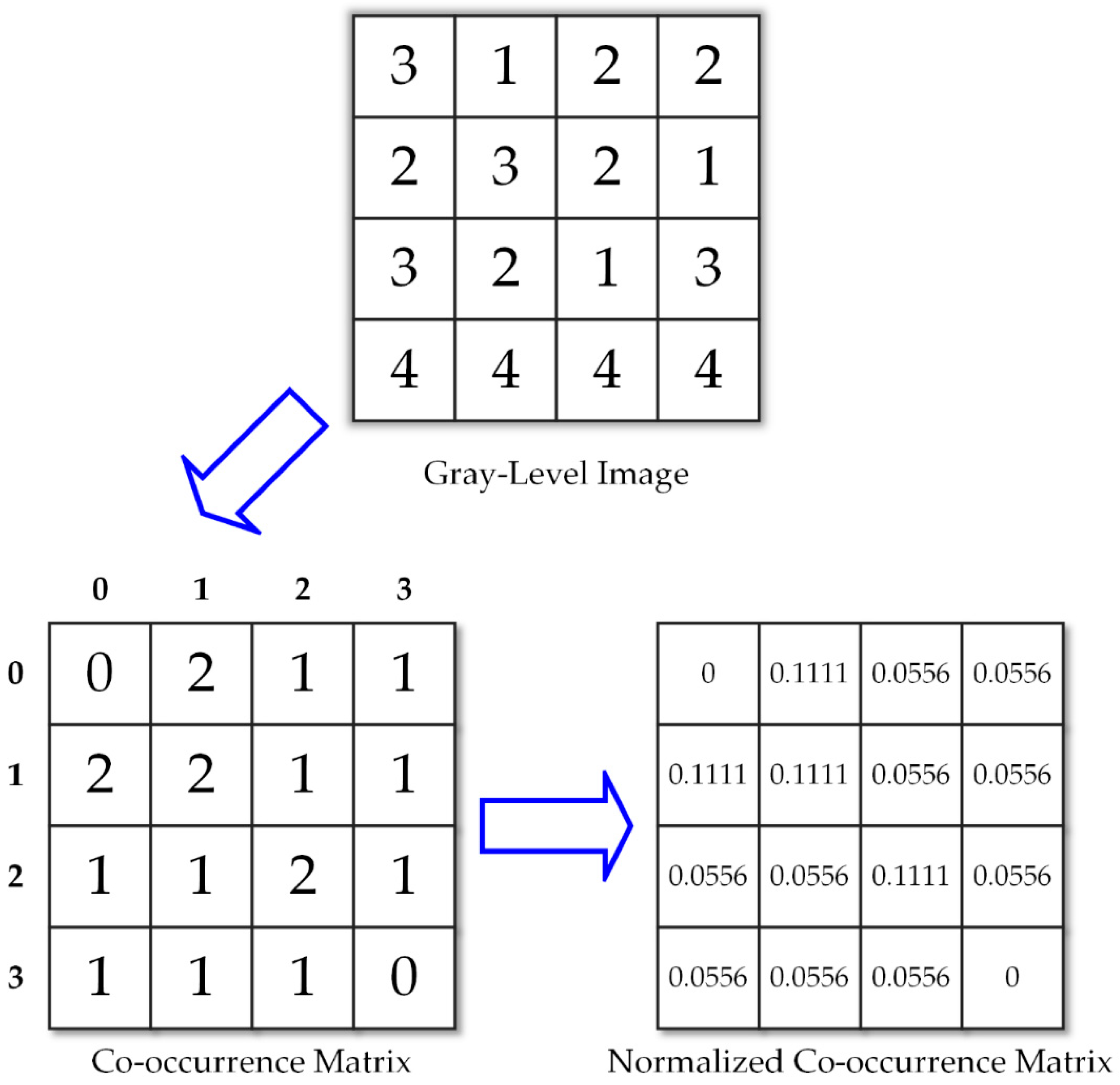
The GLCM is a matrix that shows how often the different combinations of gray levels transpire in an image. It is widely used to extract features, especially in the research of liver diseases (e.g., see [46]). In other words, it is a way of presenting the relationship between two neighboring pixels. The whole procedure to extract the Haralick features is presented as Figure 4. The co-occurrence matrix can be calculated as in Equation (1)
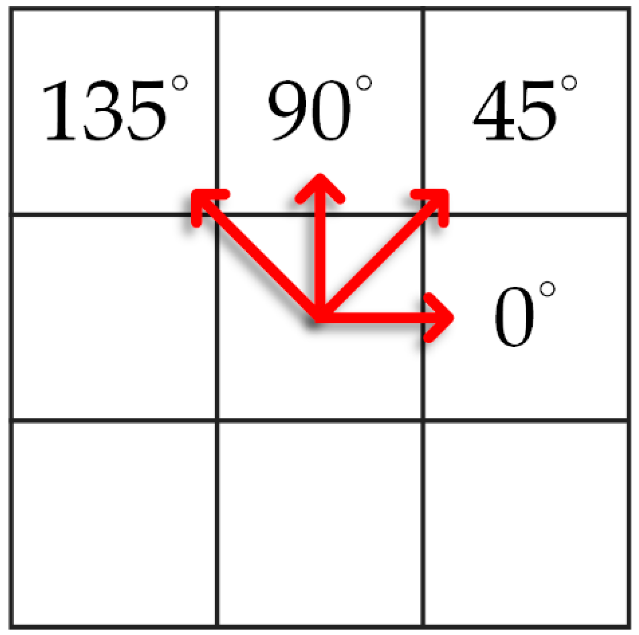
where is the number of occurrences of the pair of gray levels and , with the distance and angularity respectively; and is the intensity of a pixel in the xth row and yth column in the image. We can see that, with the different pairs , the image could be explored in different directions and distances. In this research, we choose the four directions with (illustrated in Figure 5). Thus, the pair is the nearest horizontal pixel. Moreover, there are also co-occurrence matrices for the vertical and diagonal axes .
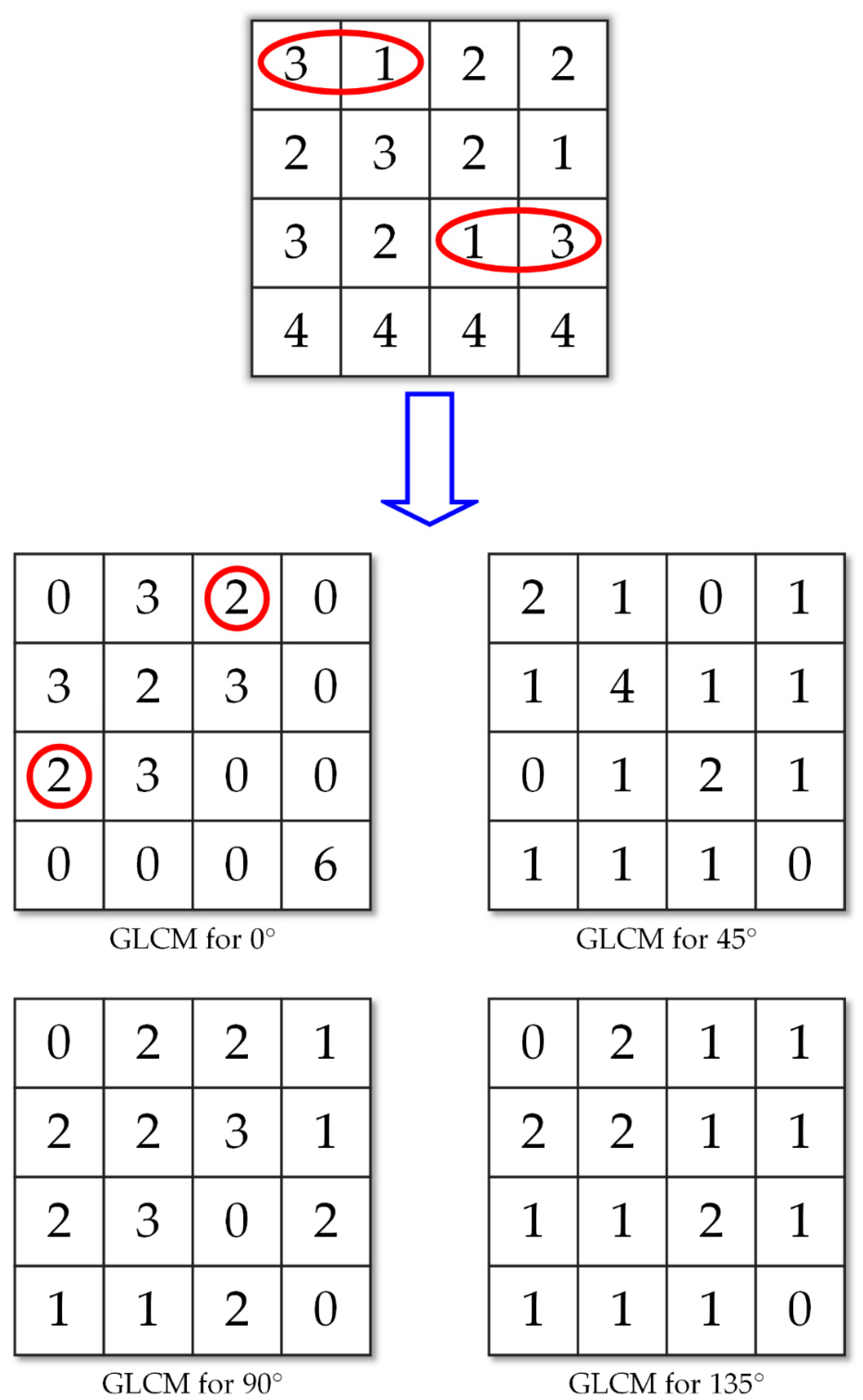
For example, in Figure 6, we calculate the gray-level co-occurrence matrix of a 4 × 4-pixel image. In this case, 3 and 1 are near each other 2 times in the image; therefore, the positions (3, 1) and (1, 3) are filled in with 2. Applying the same principle to all other pixels, we obtain the GLCM of the image.
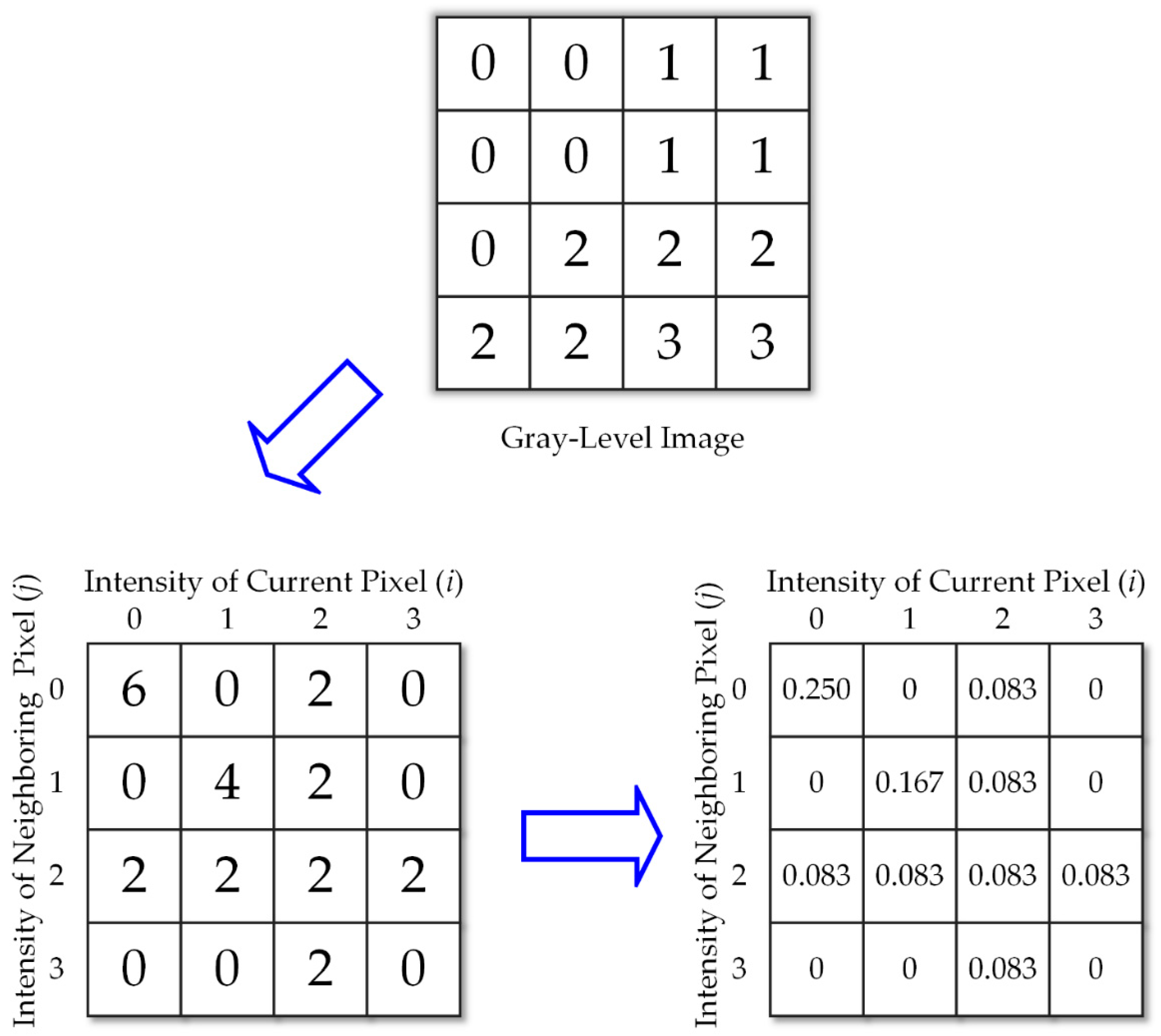
The ROI that we need to process is 32 × 32 pixels with a 256-gray level. Therefore, we will have a 256 × 256 matrix with a total of 65,536 cells; however, many cells are filled with zeros (because these combinations do not exist). This situation of many zero cells can lead to a poor approximation. The solution to this problem is that the number of gray levels is reduced, decreasing the number of zero cells, and the validity is improved considerably. In this research, the ROIs are scaled to 16 gray-level images before computing GLCM. After that, Equation (1) is normalized to be converted into a probabilistic form by Equation (2). The procedure is shown in Figure 7.
Therefore, we obtain the GLCM as in Equation (3)
From the co-occurrence matrix, the textural features proposed by Haralick are calculated.
2.2.2. Haralick Features
Thirteen features can be extracted from the GLCM for an image. These features are presented as follows:
- Energy feature:This is also called angular second moment (ASM) or uniformity. It describes the uniformity of an image. When the gray levels of pixels are similar, the energy value will be large.
- Entropy feature:This concept comes from thermodynamics, which is a field of physics concerned with heat, temperature, and their relationship with energy and work. In our case, it could be considered a chaotic or disordered quantity.
- Contrast feature:This measures the intensity variations between the pixels with a fixed direction and distance . With the same gray level, the contrast value will be equal to 0. If , there is little contrast so the weight is just 1. If , the contrast of the gray level is higher; therefore, the weight is larger at 4. This means that the weight increases exponentially.
- Correlation feature:This feature describes the linear dependency of the gray levels in the co-occurrence matrix. It shows how a center pixel relates to others.where are the mean and standard deviations, which are calculated asIn a symmetrical gray-level co-occurrence matrix, and .
- Homogeneity feature:This feature is also known as inverse difference moment (IDM). It describes the local similarity of an image.The weight of IDM is the inverse of the weight of contrast; therefore, it is lower at locations farther away from the diagonal of the GLCM. This means that positions nearer to the GLCM diagonal will have larger weights.
- Sum average feature:where
- Sum entropy feature:
- Sum variance feature:
- Difference average feature:where
- Difference variance feature:
- Difference entropy feature:
- Information measures of correlation feature 1:
- Information measures of correlation feature 2:where
2.3. GLRLM and Textural Features
The other method we use in this paper to analyze the ROIs is the GLRLM. It was first proposed by Galloway in 1975 with five features [47]. In 1990, Chu et al. [48] suggested two new features to extract gray-level information in the matrix, before Dasarathy and Holder [49] offered another four features following the idea of a joint statistical measure of gray level and run length. Tang [50] provided a good summary of some features achieved with the GLRLM.
2.3.1. GLRLM
Run-length statistics extract the coarseness of a texture in the different directions. A run is defined as a string of consecutive pixels that have the same gray level intensity along a specific linear orientation. Fine textures contain more short runs with similar gray levels, while coarse textures have more long runs with significantly different gray levels.
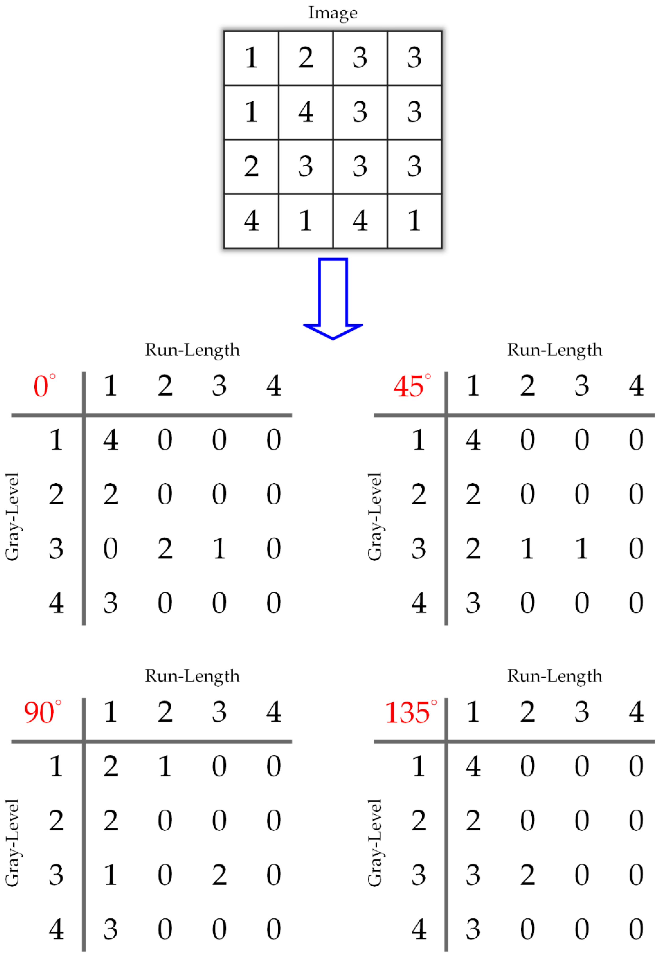
For a given image, the pair of a run-length matrix is defined as the run-number of gray level and run length , as described in Figure 9. Hence, the RLM measures how many times there are runs of j consecutive pixels with the same value, with j going from 2 to the length of the longest in a fixed orientation. Even though many GLRLMs can be defined for a given image, normally four matrices are computed, for the horizontal, vertical and diagonal directions. The matrix P has the size , where is equal to the maximum gray level and is the possible maximum run length in the corresponding image. The typical directions are 0°, 45°, 90°, and 135°, and calculating the run-length encoding for each orientation will produce a run-length matrix.
2.3.2. GLRLM Features
After a run-length matrix is calculated along a given direction, several texture descriptors are calculated to obtain the texture properties and differentiate among different textures. These descriptors can be used either with respect to each direction or by combining them if a global view of the texture information is required. Eleven features are typically extracted from the run-length matrices: short run emphasis (SRE), long run emphasis (LRE), high-gray-level run emphasis (HGRE), low-gray-level run emphasis (LGRE), pairwise combinations of the length and gray level emphasis (SRLGE, SRHGE, LRLGE, LRHGE), run-length nonuniformity (RLN), gray-level nonuniformity (GLN), and run percentage (RPC). These features describe specific characteristics in the image. For example, SRE measures the distribution of short runs in an image, while RPC measures both the homogeneity and the distribution of runs of an image in a specific direction. The formulas for calculating the features and their explanation are as follows:
- Short Run EmphasisThis describes the distribution of short runs. This value indicates how much a texture is composed of runs of short length in a given direction.where denotes the total number of runs.
- Long Run EmphasisSimilar to SRE, this describes the distribution of long runs. This value indicates how much a texture is composed of runs of long length in a given direction. These two features give more in-depth information about the coarseness of an image.
- Low-Gray-Level Run EmphasisThis describes the distribution of low gray-level values. The more low gray-level values are in an image, the larger this value is.
- High-Gray-Level Run EmphasisThis contrast, with low-gray-level run emphasis, it describes the distribution of high gray-level values. The higher gray-level values are in an image, the larger this value is.
- Short-Run Low-Gray-Level EmphasisThis describes the relative distribution of short runs and low gray-level values. The SRLGE value is large for an image with many short runs and lower gray-level values.
- Short-Run High-Gray-Level EmphasisThis describes the relative distribution of short runs and high gray-level values. The SRHGE value will be large for an image with many short runs and high gray-level values.
- Long-Run Low-Gray-Level EmphasisThis describes the relative distribution of long runs and low gray-level values. The value will be large for an image with many short runs and high gray-level values.
- Long-Run High-Gray-Level EmphasisThis describes the relative distribution of long runs and high gray-level values. The LRHGE value will be large for an image with many short runs and high gray-level values.
- Gray-Level NonuniformityThis describes the similarity of pixel values throughout the image in a given direction. It is expected to be small if the gray-level values are similar throughout the image.
- Run-Length NonuniformityThis describes the similarity of the length of runs throughout the image in a given direction. It is expected to be small if the run lengths are similar throughout the image.
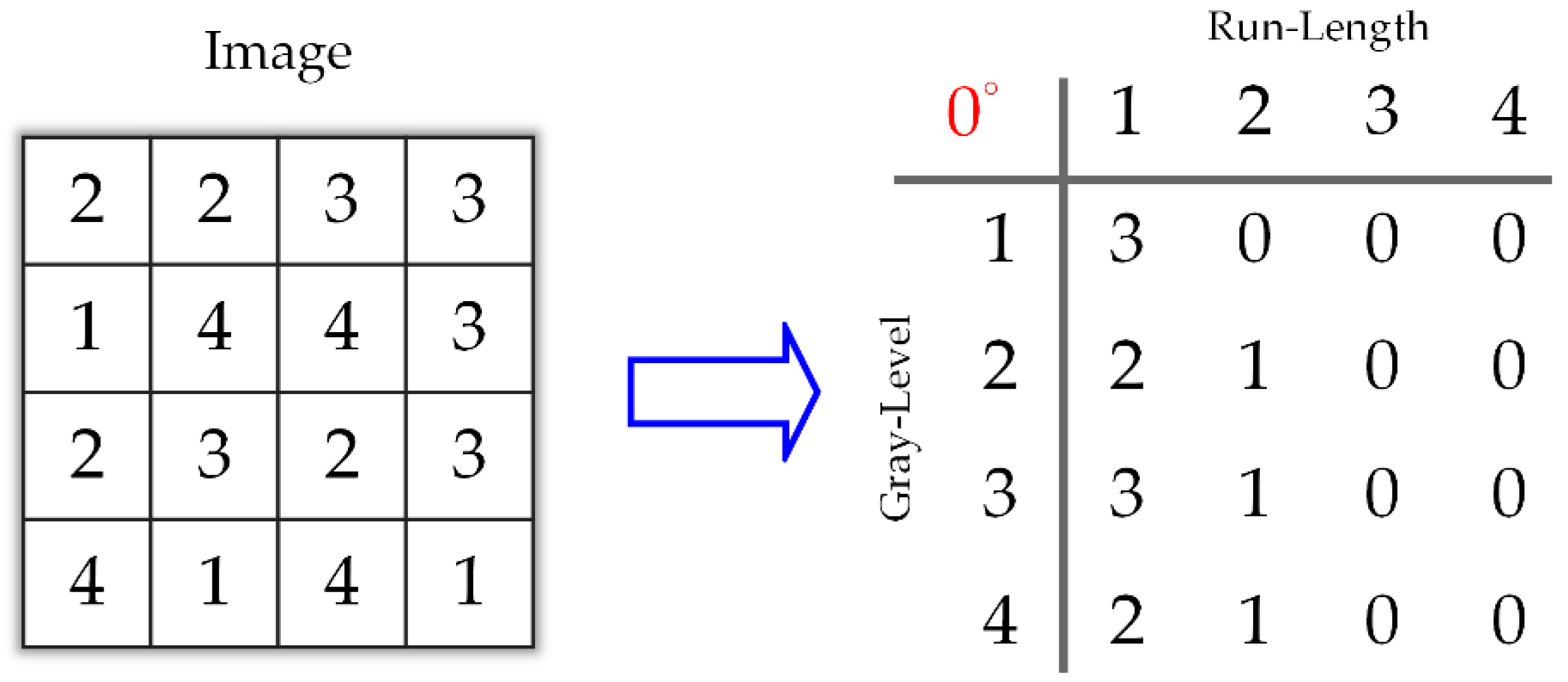
- Run PercentageThis feature is not a percentage in spite of its name. It presents the homogeneity and the distribution of runs of an image in a given direction. The RPC is the largest when the length of runs is 1 for all gray levels in a given direction.where is the number of pixels. Figure 10 shows an example calculating the GLRLM from a 4 × 4 grayscale image in the horizontal direction. We will compute 11 features following the above formulas.The results of 11 textural features, which can be computed, are shown in Table 2.
3. Feature Selection
Feature selection has been an interesting research field in machine learning, pattern recognition, data mining, and statistics. The main idea of feature selection is to eliminate redundant features that contain little or no predictive information while keeping the useful ones. To find optimal features for classification, researchers have proposed several methods to analyze the feature set. In fact, the effectiveness of features on classification is highly problem-dependent. Extracted features could perform very well for one problem but may give poor performance for others. Hence, we must pick proper features for the given problem at hand. Ultimately, from various feature extraction methods, we need to find a set of features that is optimal for the problem. In this research, we use sequential forward selection (SFS) [52,53], sequential backward selection (SBS) [53,54], and F-score [55] to find the optimal feature subset.
3.1. Sequential Forward Selection (SFS)
SFS [52,53] begins by evaluating all samples of a dataset that consist of only one input attribute. In other words, we start from the empty set and sequentially add feature , which results in the highest-valued objective function . Its algorithm can be broken down into the following steps:
- Step 1: Start with empty set .
- Step 2: Select the next best feature with . In our case, the objective function is based on the classification rate from a cross-validation test. The mean value of a 10-fold cross-validation test is used to evaluate the feature subset.
- Step 3: Update = and set .
- Step 4: Go to Step 2.
This procedure continues until a predefined number of features are selected. According to the above process, we see that the search space is drawn such as an ellipse to emphasize the fact that there are fewer states towards the full or empty sets. To find the optimum input feature set overall, the easiest means is an exhaustive search. However, this is very expensive. Compared with an exhaustive search, forward selection is much cheaper. SFS works best when the optimal subset has a small number of features, and the main disadvantage of SFS is that it is unable to remove features that become obsolete after the addition of other features.
3.2. Sequential Backward Selection (SBS)
Contrary to SFS, SBS [53,54] works in the opposite way. SBS starts from a full set of features and sequentially eliminates the worst feature to result in the highest-valued objective function . Its algorithm can be broken down into the following steps:
- Step 1: Start with full set
- Step 2: Eliminate the worst feature with . The objective function is based on the classification rate from a cross-validation test. The mean value of the 10-fold cross-validation test is used to evaluate the feature subset.
- Step 3: Update = and set .
- Step 4: Go to Step 2.
This procedure continues until a predefined number of features are left. SBS usually works best when the optimal feature subset has a large number of features since SBS spends most of its time visiting large subsets.
3.3. F-Score
F-score [55] is a technique that measures discrimination. Given training vectors , , if the number of positive and negative instances are and , respectively, then the F-score of the ith feature is calculated as in Equation (41)
where are the averages of the ith features of the whole, positive, and negative data, respectively, and are the ith features of the kth positive and negative sample, respectively. F-score indicates the discrimination between the positive and negative sets; therefore, the larger the F-score, the more likely this feature is to be more discriminative. Thus, we could consider this score as a criterion for feature selection. A disadvantage of this method is that it cannot reveal shared information between features [55]. In the example, both features have low values of F-score; however, the set of them classifies the two groups precisely.
In spite of this drawback, F-score is simple and generally quite effective. We order all features based on F-score and then use a classifier to train/test the set that includes the feature with the highest F-score. Then, we add the second highest F-score feature to the feature set before training and testing all of the dataset again. The procedure is repeated until all features are added to the feature set.
4. SVM Classification
Support vector machine (SVM), which was proposed by Vapnik et al. [37], is a powerful machine learning method based on statistical learning theory. Its theory is based on the idea of finding an optimal hyperplane to separate two classes. This produces a classifier that performs well on unseen patterns. SVM has been widely applied in many fields, such as regression estimation, environment illumination learning, object recognition, and bioinformatics analysis. In each case, there are usually many possible hyperplanes to separate the groups; however, there is only one hyperplane that has a maximal margin.
In this research, two liver diseases need to be distinguished. Hence, LIBSVM, a popular machine learning tool for classification, regression, and other machine learning tasks, was used to implement a multiclass learning task. LIBSVM, which was proposed by Lin et al. [38], is a library for support vector machines. It is an integrated library for support vector classification (C-SVC, nu-SVC) and distribution estimation (one-class SVM). A typical use of LIBSVM includes two steps: the first step is training a data set to obtain a model and the second is to use the model to predict the information of a testing data set.
5. Performance Evaluation
To reduce the variability of the prediction performance, a cross-validation test is usually used to evaluate the performance of the proposed system. It is one of the most popular methods to evaluate a model’s prediction performance. If a model was trained and tested on the same data, it would easily lead to an overoptimistic result. Therefore, the better approach, the holdout method, is to split the training data into disjoint subsets.
As it is a single train-and-test method, the error rate we got resulted from an ‘unfortunate’ split. Moreover, in some cases of a lack of samples, we cannot afford the luxury of setting. The drawbacks of the holdout can be overcome with a family of resampling methods, called cross-validation. Two well-known kinds of cross-validation are leave-one-out cross-validation (LOOCV) and k-fold cross-validation.
In k-fold cross-validation, the total samples are randomly partitioned into k groups, which have the same size. Of the k groups, one group is for testing the model, while the remaining (k − 1) groups are used as training data. This process is repeated k times (the folds) until all groups are tested. Then, the results from the k experiments can be averaged to produce a single estimation. Thus, the true accuracy is estimated as the average accuracy rate
The advantage of this method is that all samples are used for both training and validation, and each observation is used for validation only one time. Although 10-fold and 5-fold cross-validation are commonly used, in general k is an unfixed parameter.
Leave-one-out cross-validation could be considered a degenerate case of k-fold cross-validation where k is the total number of samples. Consequently, for a data set with N samples, LOOCV performs N experiments. In each experiment, only one sample is used for testing, while N-1 samples left are for the training process.
In this research, we use 10-fold cross-validation for performance evaluation. The classification results in four kinds of value: true positive (TP), true negative (TN), false positive (FP), and false negative (FN) (shown in Table 3).
Where ‘true’ and ‘false’ are intended for result correction, while ‘positive’ or ‘negative’ signifies the tumor is either HCC or liver abscess. Based on the information, we calculate the accuracy factors as in Equation (43), which describes the performance of classifiers
6. Experimental Results and Discussion
6.1. Result and Discussion
Various experiments were conducted. Two kinds of feature matrices (GLCM and GLRLM) were calculated and selected by the feature selection methods (sequential forward selection, sequential backward selection, and F-score) before being classified by the support vector machine. The following sections will present the results of the different combinations for considering the optimal methods for a CAD system.
6.1.1. Classification by All Features
As mentioned in the previous parts, we extracted 96 features from a region of interest (ROI). They consisted of many characteristics of each kind of liver disease. In this experiment, SVM was used to discriminate the diseases by using each kind of feature (GLCM or GLRLM) and using the two kinds (GLCM and GLRLM) together. Table 4 shows the results of classification in this case.
As seen from Table 4, the classification results without applying any feature selection method of SVM are not accurate enough, except using the model that included GLCM and SVM, whose highest accuracy rate is 75.75%. The other combinations of SVM obtain detection rates of 54.53% and 61%.
This result shows that both GLCM and GLRLM features can be applied to classification of HCC and liver abscess; however, GLRLM seems to contain more noise than GLCM. The classification can adapt to the redundant features in both GLCM and GLRLM; however, SVM’s performance is affected significantly. In the next section, the classification was conducted by applying sequential forward selection.
6.1.2. Classification by Using Sequential Forward Selection
After applying sequential forward selection for the different kinds of feature set, different numbers of features were selected. The results are shown in Table 5. In SVM classification, we set one more condition for the SFS process. That is, the lower bound of selected features is four features because if the number of selected features is not large enough, the result of classification will be not good. For example, the process of SVM, which is used to train and test all samples with only one feature, only takes approximately 0.3 s.
Regarding SVM, we see that SFS gives a slight improvement from 75.75% to 78% with GLCM, a significant change in the recognition rate with GLRLM from 54.53% to 88.13%, and an improvement with the combination of GLCM and GLRLM from 61% to 89.25%.
6.1.3. Classification by Using Sequential Backward Selection
After conducting sequential backward selection, we obtain the results shown in Table 6. It is obvious that SBS enhances the accuracy of all methods to different levels. In case of GLCM features, the accuracy is slightly decreased by 0.25% with SVM. For GLRLM and the combination between GLCM and GLCM, the highest result is achieved by SVM and the GLCM-GLRLM combination with SBS (88.87%). This is followed by 88.25% with the model that used GLRLM and SVM.
6.1.4. F-Score
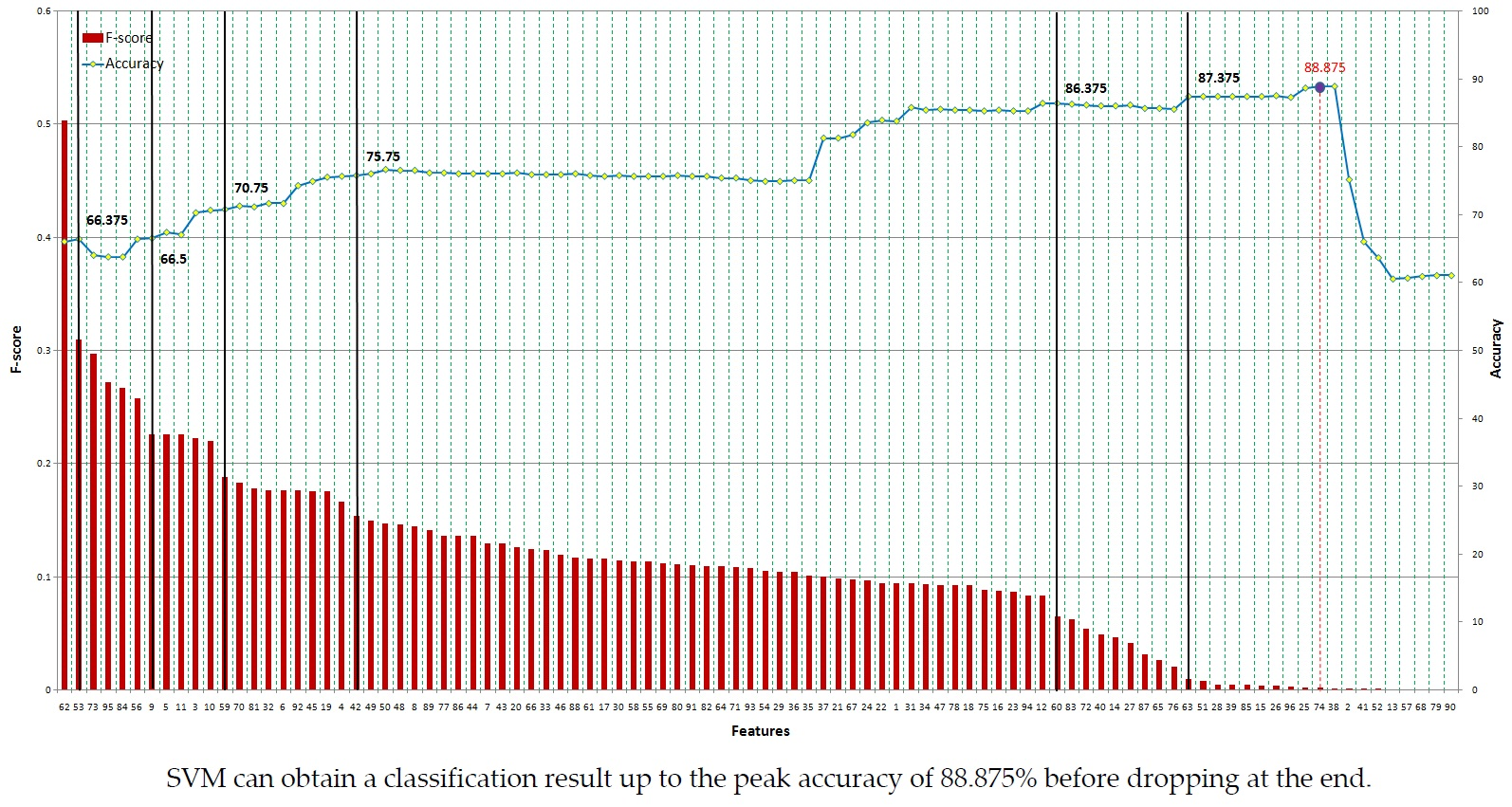
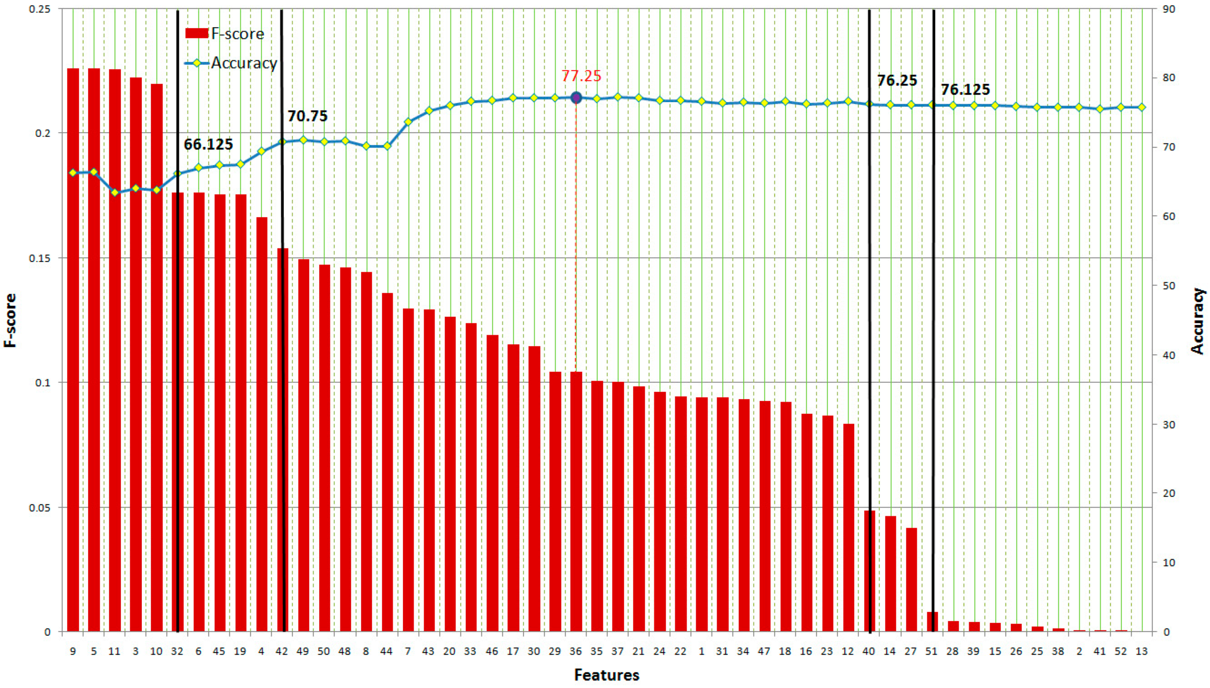
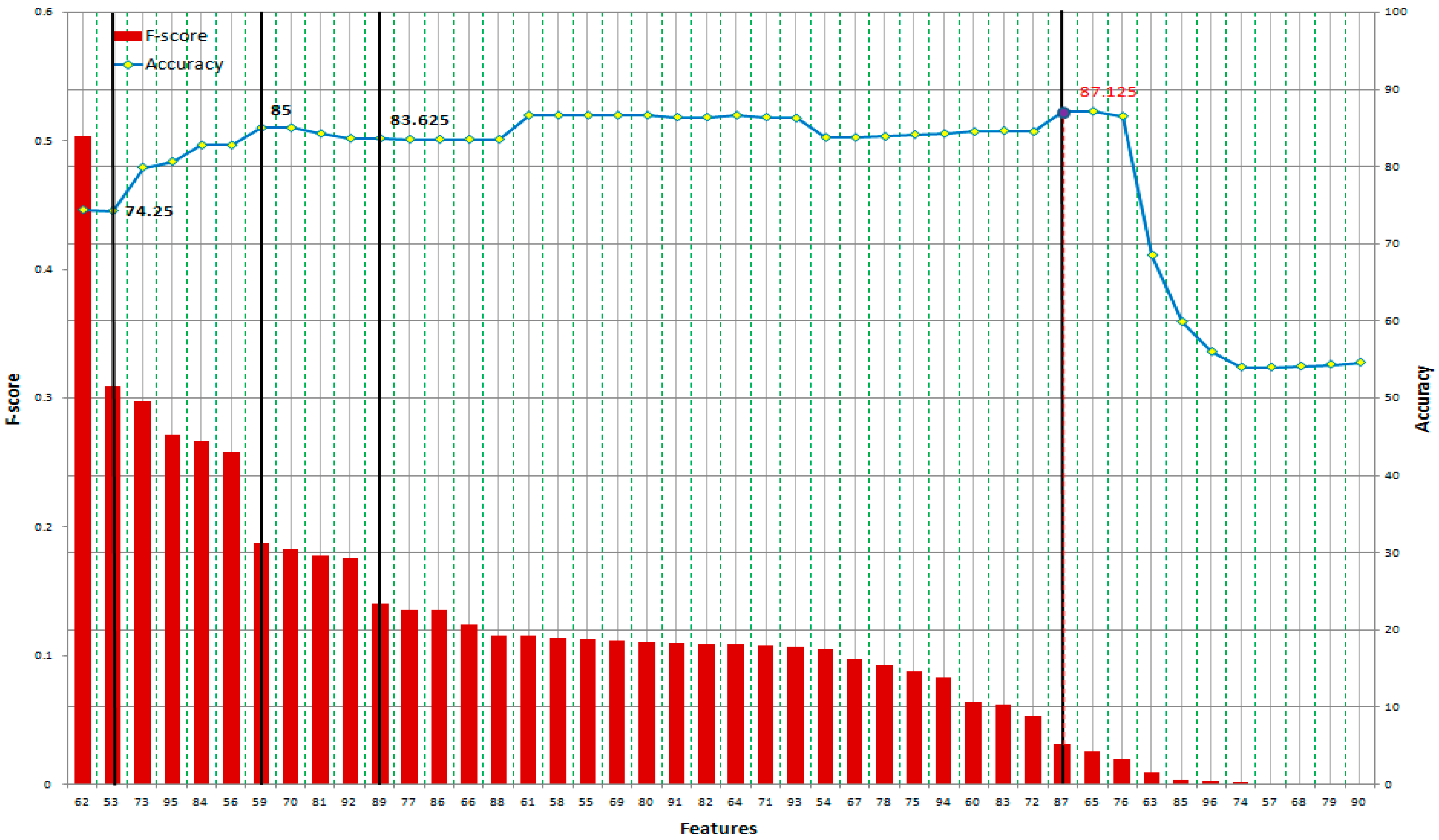
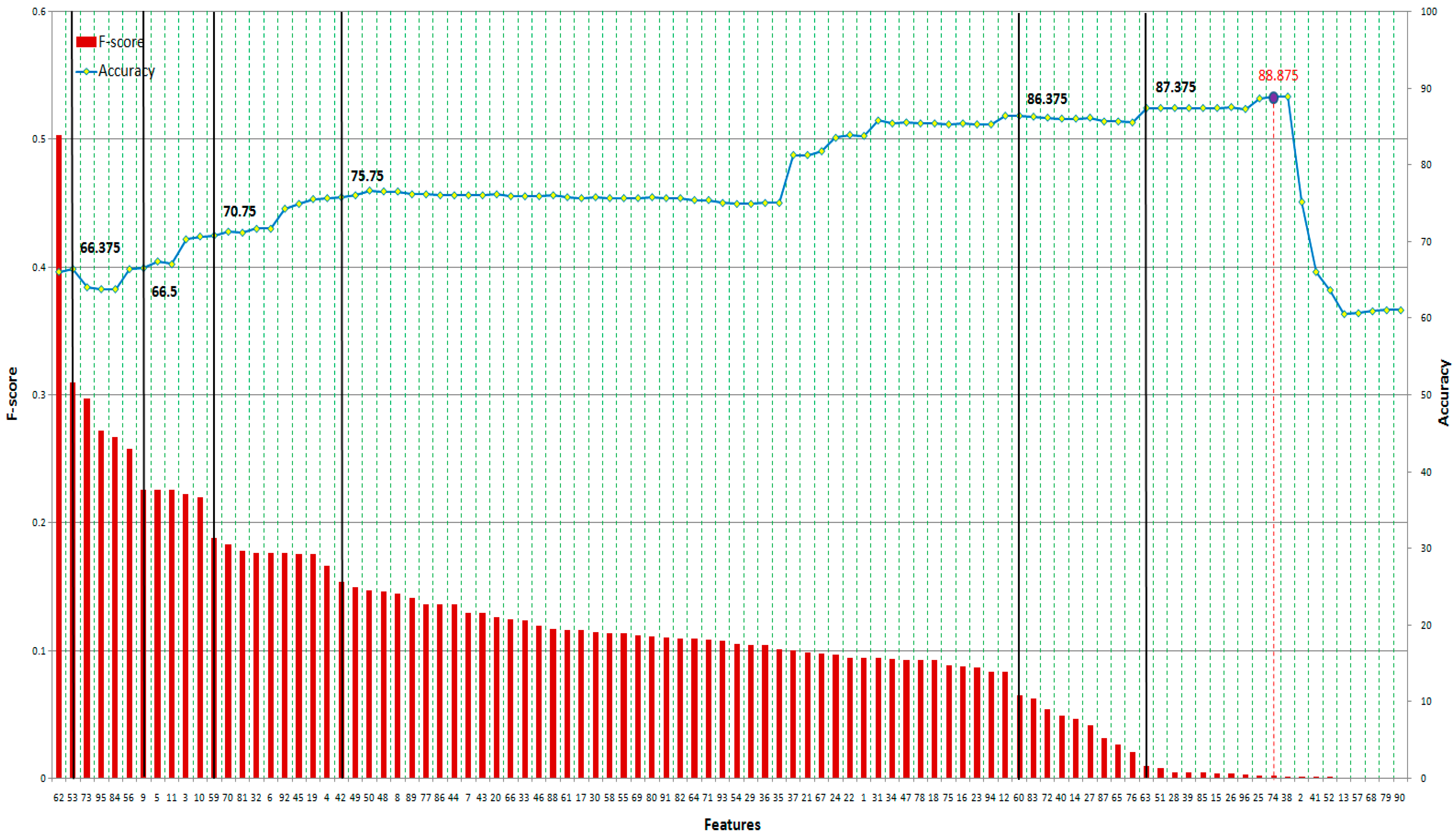
Based on Equation (41), the F-score of each feature can be computed (shown in Table 7 and Table 8). As shown in Figure 11, when we add more GLCM features based on their F-score, the accuracy increases and reaches a peak at the 36th feature at 77.25% accuracy and then slightly decreases at the end. Meanwhile, SVM achieves 87.125% accuracy at the 87th feature (including 34 features) before dropping rapidly from the 63rd feature to the end of GLRLM features, as shown in Figure 12. In this case, we can also obtain 86.625% accuracy with only 16 features at the 61st feature of GLRLM. When using all features, the trend of accuracy is quite similar to the case of applying GLRLM features. SVM can obtain a classification result up to the peak accuracy of 88.875% before dropping at the end, as shown in Figure 13.
The other method to apply F-score is to select several thresholds where the gap between low F-score and high F-score is considerable. We selected four thresholds for each kind of feature and six thresholds for all features. The results are shown in Table 9.
As presented in Table 9, the threshold method achieves results as good as those by searching all features.
6.2. Performance Analysis
The performance of all methods is summarized in Table 10. The models using SVM and GLRLM or all features with any selection method give the highest accuracy, approximately 88%. For example, SVM tried all cases of feature sets based on F-score for approximately 40 s. Finally, the highest accuracy obtained by the model, which contains SVM and all features selected by SFS, is 89.25%. Nevertheless, in case of reducing the processing load, the threshold of F-score for SVM could be considered because it also gives a good performance. It took only 1.8 s to achieve the classification rate of 87.375%, compared with 40 s for SFS. These differences will have significant meaning for processing a large dataset.
7. Conclusions
Hepatocellular carcinoma (HCC) and liver abscess are among the most dangerous liver diseases worldwide. Due to the need to diagnose liver disease based on ultrasound images, developing a computer-aided diagnosis (CAD) system will greatly assist inexperienced physicians in their decision making. Therefore, this research proposes a system to reduce the erroneous classification of HCC and liver abscess. First, 96 textural features including 52 features of the gray-level co-occurrence matrix (GLCM) and 44 features of the gray-level run-length matrix (GLRLM) were extracted from the regions of interest (ROIs), which were verified by radiologists and recognized by biopsy. To obtain the important features, we applied the following three feature selection schemes: (i) sequential forward selection (SFS), (ii) sequential backward selection (SBS), and (iii) F-score. Then we determined the most discriminative feature set. Finally, the support vector machine (SVM) classifier was trained from the features of the training set and tested by 10-fold cross-validation to obtain a reliable result. The final results show that the proposed methods for a CAD system can provide diagnostic help while distinguishing HCC from liver abscess with high accuracy (up to 89.25%) of identification.
Author Contributions
Conceptualization, S.S.-D.X., C.-C.C. and C.-T.S.; Formal analysis, S.S.-D.X., C.-C.C., C.-T.S. and P.Q.P.; Funding acquisition, S.S.-D.X., C.-C.C. and C.-T.S.; Investigation, S.S.-D.X., C.-C.C., C.-T.S. and P.Q.P.; Methodology, S.S.-D.X., C.-C.C., C.-T.S. and P.Q.P.; Project administration, S.S.-D.X. and C.-T.S.; Resources, C.-C.C. and C.-T.S.; Software, P.Q.P.; Supervision, S.S.-D.X.; Validation, S.S.-D.X. and P.Q.P.; Visualization, C.-C.C. and C.-T.S.; Writing—original draft, S.S.-D.X., C.-C.C., C.-T.S. and P.Q.P.; Writing—review & editing, S.S.-D.X., C.-C.C., C.-T.S. and P.Q.P.
Acknowledgments
This research was supported in part by Taipei Medical University (TMU), Taiwan, and National Taiwan University of Science and Technology (NTUST), Taiwan, under the Grants TMU-NTUST-100-11, TMU-NTUST-101-10, and TMU-NTUST-103-12, and by the Ministry of Science and Technology (MOST), Taiwan, under the Grant MOST 107-2221-E-011-145.
Conflicts of Interest
The authors declare no conflict of interest.
References
- Pisani, P.; Parkin, D.M.; Bray, F.; Ferlay, J. Estimates of the worldwide mortality from 25 cancers in 1990. Int. J. Cancer 1999, 83, 18–29. [Google Scholar] [CrossRef] [Green Version]
- Tang, A.; Cloutier, G.; Szeverenyi, N.M.; Sirlin, C.B. Ultrasound elastography and MR elastography for assessing liver fibrosis: Part 1, principles and techniques. Am. J. Roentgenol. 2015, 205, 22–32. [Google Scholar] [CrossRef]
- Tang, A.; Cloutier, G.; Szeverenyi, N.M.; Sirlin, C.B. Ultrasound elastography and MR elastography for assessing liver fibrosis: Part 2, diagnostic performance, confounders, and future directions. Am. J. Roentgenol. 2015, 205, 33–40. [Google Scholar] [CrossRef] [PubMed]
- Tai, C.-J.; Huang, M.-T.; Wu, C.-H.; Tai, C.-J.; Shi, Y.-C.; Chang, C.-C.; Chang, Y.-J.; Kuo, L.-J.; Wei, P.-L.; Chen, R.-J.; et al. Contrast-enhanced ultrasound and computed tomography assessment of hepatocellular carcinoma after transcatheter arterial chemo-embolization: A systematic review. J. Gastrointest. Liver Dis. 2016, 25, 499–507. [Google Scholar]
- Mozumi, M.; Hasegawa, H. Adaptive beamformer combined with phase coherence weighting applied to ultrafast ultrasound. Appl. Sci. 2018, 8, 204. [Google Scholar] [CrossRef]
- Albinsson, J.; Hasegawa, H.; Takahashi, H.; Boni, E.; Ramalli, A.; Ahlgren, Å.R.; Cinthio, M. Iterative 2D tissue motion tracking in ultrafast ultrasound Imaging. Appl. Sci. 2018, 8, 662. [Google Scholar] [CrossRef]
- Chen, S.-H.; Peng, C.-Y. Ultrasound-based liver stiffness surveillance in patients treated for chronic hepatitis B or C. Appl. Sci. 2018, 8, 626. [Google Scholar] [CrossRef]
- Luchies, A.C.; Byram, B.C. Deep neural networks for ultrasound beamforming. IEEE Trans. Med. Imaging 2018, 37, 2010–2021. [Google Scholar] [CrossRef]
- Kijanka, P.; Qiang, B.; Song, P.; Carrascal, C.A.; Chen, S.; Urban, M.W. Robust phase velocity dispersion estimation of viscoelastic materials used for medical applications based on the multiple signal classification method. IEEE Trans. Ultrason. Ferroelectr. Freq. Control 2018, 65, 423–439. [Google Scholar] [CrossRef]
- Nelson, R.C. Techniques for computed tomography of the liver. Radiol. Clin. N. Am. 1991, 29, 1199–1212. [Google Scholar]
- Sistrom, L.; Gay, S.B.; Holder, C.A. Methods used for liver computed tomography scanning in community radiology practice. Investig. Radiol. 1993, 28, 1139–1143. [Google Scholar] [CrossRef]
- Gotra, A.; Sivakumaran, L.; Chartrand, G.; Vu, K.-N.; Vandenbroucke-Menu, F.; Kauffmann, C.; Kadoury, S.; Gallix, B.; Guise, J.A.; Tang, A. Liver segmentation: Indications, techniques and future directions. Insights Imaging 2017, 8, 377–392. [Google Scholar] [CrossRef] [PubMed]
- Balagourouchetty, L.; Pragatheeswaran, J.K.; Pottakkat, B.; Govindarajalou, R. Enhancement approach for liver lesion diagnosis using unenhanced CT images. IET Comput. Vis. 2018, 12, 1078–1087. [Google Scholar] [CrossRef]
- Li, S.; Jiang, H.; Yao, Y.-D.; Yang, B. Organ location determination and contour sparse representation for multiorgan segmentation. IEEE J. Biomed. Health Inform. 2018, 22, 852–861. [Google Scholar] [CrossRef] [PubMed]
- Marvasti, N.B.; Yörük, E.; Acar, B. Computer-aided medical image annotation: Preliminary results with liver lesions in CT. IEEE J. Mag. 2018, 22, 1561–1570. [Google Scholar] [CrossRef] [PubMed]
- Seregni, M.; Paganelli, C.; Summers, P.; Bellomi, M.; Baroni, G.; Riboldi, M. A hybrid image registration and matching framework for real-time motion tracking in MRI-guided radiotherapy. IEEE Trans. Biomed. Eng. 2018, 61, 131–139. [Google Scholar] [CrossRef]
- Jabarulla, Y.; Lee, H.-N. Computer aided diagnostic system for ultrasound liver images: A systematic review. Optik 2017, 140, 1114–1126. [Google Scholar] [CrossRef]
- Huang, Q.; Zhang, F.; Li, X. Machine learning in ultrasound computer-aided diagnostic systems: A survey. BioMed Res. Int. 2018, 2018, 5137904. [Google Scholar] [CrossRef]
- Nicholas, D.; Nassiri, D.; Garbutt, P.; Hill, C. Tissue characterization from ultrasound B-scan data. Ultrasound Med. Biol. 1986, 12, 135–143. [Google Scholar] [CrossRef]
- Richard, W.D.; Keen, C.G. Automated texture-based segmentation of ultrasound images of the prostate. Comput. Med. Imaging and Graph. 1996, 20, 131–140. [Google Scholar] [CrossRef]
- Pavlopoulos, S.; Konnis, G.; Kyriacou, E.; Koutsouris, D.; Zoumpoulis, P.; Theotokas, I. Evaluation of texture analysis techniques for quantitative characterization of ultrasonic liver images. In Proceedings of the 18th Annual International Conference of the IEEE, Amsterdam, The Netherlands, 31 October–3 November 1996; pp. 1151–1152. [Google Scholar]
- Bleck, J.; Ranft, U.; Gebel, M.; Hecker, H.; Westhoff-Bleck, M.; Thiesemann, C.; Wagner, S.; Manns, M. Random field models in the textural analysis of ultrasonic images of the liver. IEEE Trans. Med. Imaging 1996, 15, 796–801. [Google Scholar] [CrossRef] [PubMed]
- Kadah, Y.M.; Farag, A.A.; Zurada, J.M.; Badawi, A.M.; Youssef, A. Classification algorithms for quantitative tissue characterization of diffuse liver disease from ultrasound images. IEEE Trans. Med. Imaging 1996, 15, 466–478. [Google Scholar] [CrossRef] [PubMed]
- Gebbinck, M.K.; Verhoeven, J.; Thijssen, J.; Schouten, T.E. Application of neural networks for the classification of diffuse liver disease by quantitative echography. Ultrason. Imaging 1993, 15, 205–217. [Google Scholar] [CrossRef]
- Pavlopoulos, S.; Kyriacou, E.; Koutsouris, D.; Blekas, K.; Stafylopatis, A.; Zoumpoulis, P. Fuzzy neural network-based texture analysis of ultrasonic images. IEEE Eng. Med. Biol. Mag. 2000, 19, 39–47. [Google Scholar] [CrossRef] [PubMed]
- Horng, M.-H.; Sun, Y.-N.; Lin, X.-Z. Texture feature coding method for classification of liver sonography. Comput. Med. Imaging Graph. 2002, 26, 33–42. [Google Scholar] [CrossRef]
- Yang, P.-M.; Chen, C.-M.; Lu, T.-W.; Yen, C.-P. Computer-aided diagnosis of sonographic liver cirrhosis: A spleen-reference approach. Med. Phys. 2008, 35, 1180–1190. [Google Scholar] [CrossRef] [PubMed]
- Laghi, A.; Iannaccone, R.; Rossi, P.; Carbone, I.; Ferrari, R.; Mangiapane, F.; Nofroni, I.; Passariello, R. Hepatocellular carcinoma: Detection with triple-phase multi–detector row helical CT in patients with chronic hepatitis. Radiology 2003, 226, 543–549. [Google Scholar] [CrossRef]
- Choi, B.I. The current status of imaging diagnosis of hepatocellular carcinoma. Liver Transplant. 2004, 10, S20–S25. [Google Scholar] [CrossRef] [Green Version]
- Pérez, J.A.A.; González, J.J.; Baldonedo, R.F.; Sanz, L.; Carreño, G.; Junco, A.; Rodríguez, J.I.; Martínez, M.D.; Jorge, J.I. Clinical course, treatment, and multivariate analysis of risk factors for pyogenic liver abscess. Am. J. Surg. 2001, 181, 177–186. [Google Scholar] [CrossRef]
- Cruz-Gomez, C.; Wiederhold, P.; Gudino-Zayas, M. Automatic liver tissue segmentation in microscopic images using fusion color space and multiscale morphological reconstruction. In Proceedings of the International Conference on Technological Advances in Electrical, Electronics and Computer Engineering (TAEECE), Konya, Turkey, 9–11 May 2013; pp. 88–92. [Google Scholar]
- Jiang, Z.; Yamauchi, K.; Yoshioka, K.; Aoki, K.; Kuroyanagi, S.; Iwata, A.; Yang, J.; Wang, K. Support vector machine-based feature selection for classification of liver fibrosis grade in chronic hepatitis C. J. Med. Syst. 2006, 30, 389–394. [Google Scholar] [CrossRef]
- Sabih, D.; Hussain, M. Automated classification of liver disorders using ultrasound images. J. Med. Syst. 2012, 36, 3163–3172. [Google Scholar]
- Hatt, R.; Ng, G.; Parthasarathy, V. Enhanced needle localization in ultrasound using beam steering and learning-based segmentation. Comput. Med. Imaging Graph. 2015, 41, 46–54. [Google Scholar] [CrossRef] [PubMed]
- Ribeiro, R.T.; Marinho, R.T.; Sanches, J.M. An ultrasound-based computer-aided diagnosis tool for steatosis detection. IEEE J. Biomed. Health Inform. 2014, 18, 1397–1403. [Google Scholar] [CrossRef] [PubMed]
- Moldovanu, S.; Moraru, L.; Bibicu, D. Computerized decision support in liver steatosis investigation. Int. J. Biol. Biomed. Eng. 2012, 6, 69–76. [Google Scholar]
- Vapnik, V. Estimation of Dependences Based on Empirical Data; Nauka: Moscow, Russia, 1979; (English Translation: Springer: New York, NY, USA, 1982). [Google Scholar]
- Fan, R.-E.; Chen, P.-H.; Lin, C.-J. Working set selection using second order information for training support vector machines. J. Mach. Learn. Res. 2005, 6, 1889–1918. [Google Scholar]
- Virmani, J.; Kumar, V.; Kalra, N.; Khandelwal, N. PCA−SVM based CAD system for focal liver lesions using B-Mode ultrasound images. Def. Sci. J. 2013, 63, 478–486. [Google Scholar] [CrossRef]
- Sakr, A.; Fares, M.E.; Ramadan, M. Automated focal liver lesion staging classification based on Haralick texture features and Multi-SVM. Int. J. Comput. Appl. 2014, 91, 17–25. [Google Scholar]
- Mittal, D.; Rani, A. Detection and classification of focal liver lesions using support vector machine classifiers. J. Biomed. Eng. Med. Imaging 2016, 3, 21. [Google Scholar]
- Haralick, R.M.; Shanmugam, K.; Dinstein, I.H. Textural features for image classification. IEEE Trans. Syst. Man Cybern. 1973, 610–621. [Google Scholar] [CrossRef]
- Poonguzhali, S.; Ravindran, G. Automatic classification of focal lesions in ultrasound liver images using combined texture features. Inf. Technol. J. 2008, 7, 205–209. [Google Scholar] [CrossRef]
- Gomez, W.; Pereira, W.C.A.; Infantosi, A.F.C. Analysis of co-occurrence texture statistics as a function of gray-level quantization for classifying breast ultrasound. IEEE Trans. Med. Imaging 2012, 31, 1889–1899. [Google Scholar] [CrossRef] [PubMed]
- Onal, S.; Lai-Yuen, S.K.; Bao, P.; Weitzenfeld, A.; Hart, S. MRI-based segmentation of pubic bone for evaluation of pelvic organ prolapse. IEEE J. Biomed. Health Inform. 2014, 18, 1370–1378. [Google Scholar] [CrossRef] [PubMed]
- Yi, G.; Yuanyuan, W.; Dehong, K.; Xianhong, S. Automatic classification of intracardiac tumor and thrombi in echocardiography based on sparse representation. Biomed. Health Inform. IEEE J. 2015, 19, 601–611. [Google Scholar]
- Galloway, M.M. Texture analysis using gray level run lengths. Comput. Graph. Image Process. 1975, 4, 172–179. [Google Scholar] [CrossRef]
- Chu, A.; Sehgal, C.M.; Greenleaf, J.F. Use of gray value distribution of run lengths for texture analysis. Pattern Recognit. Lett. 1990, 11, 415–419. [Google Scholar] [CrossRef]
- Dasarathy, V.; Holder, E.B. Image characterizations based on joint gray level-run length distributions. Pattern Recognit. Lett. 1991, 12, 497–502. [Google Scholar] [CrossRef]
- Tang, X. Texture information in run-length matrices. IEEE Trans. Image Process. 1998, 7, 1602–1609. [Google Scholar] [CrossRef]
- Mitrea, D.; Nedevschi, S.; Lupsor, M.; Socaciu, M.; Badea, R. Experimenting various classification techniques for improving the automatic diagnosis of the malignant liver tumors, based on ultrasound images. In Proceedings of the International Congress on Image and Signal Processing (CISP), Yantai, China, 16–18 October 2010; pp. 1853–1858. [Google Scholar]
- Marill, T.; Green, D.M. On the effectiveness of receptors in recognition system. IEEE Trans. Inform. Theory 1963, 9, 11–17. [Google Scholar] [CrossRef]
- Pudil, P.; Novovičová, J.; Kittler, J. Floating search methods in feature selection. Pattern Recognit. Lett. 1994, 15, 1119–1125. [Google Scholar] [CrossRef]
- Whitney, A.W. A direct method of nonparametric measurement selection. IEEE Trans. Comput. 1971, 20, 1100–1103. [Google Scholar] [CrossRef]
- Chen, Y.-W.; Lin, C.-J. Combining SVMs with various feature selection strategies. In Feature Extraction: Foundations and Applications; Springer: Berlin/Heidelberg, Germany, 2006; Chapter 12; pp. 315–324. [Google Scholar]
Figure 1.
An example of the cropping process for the original US image.

Figure 2.
The cropping window.

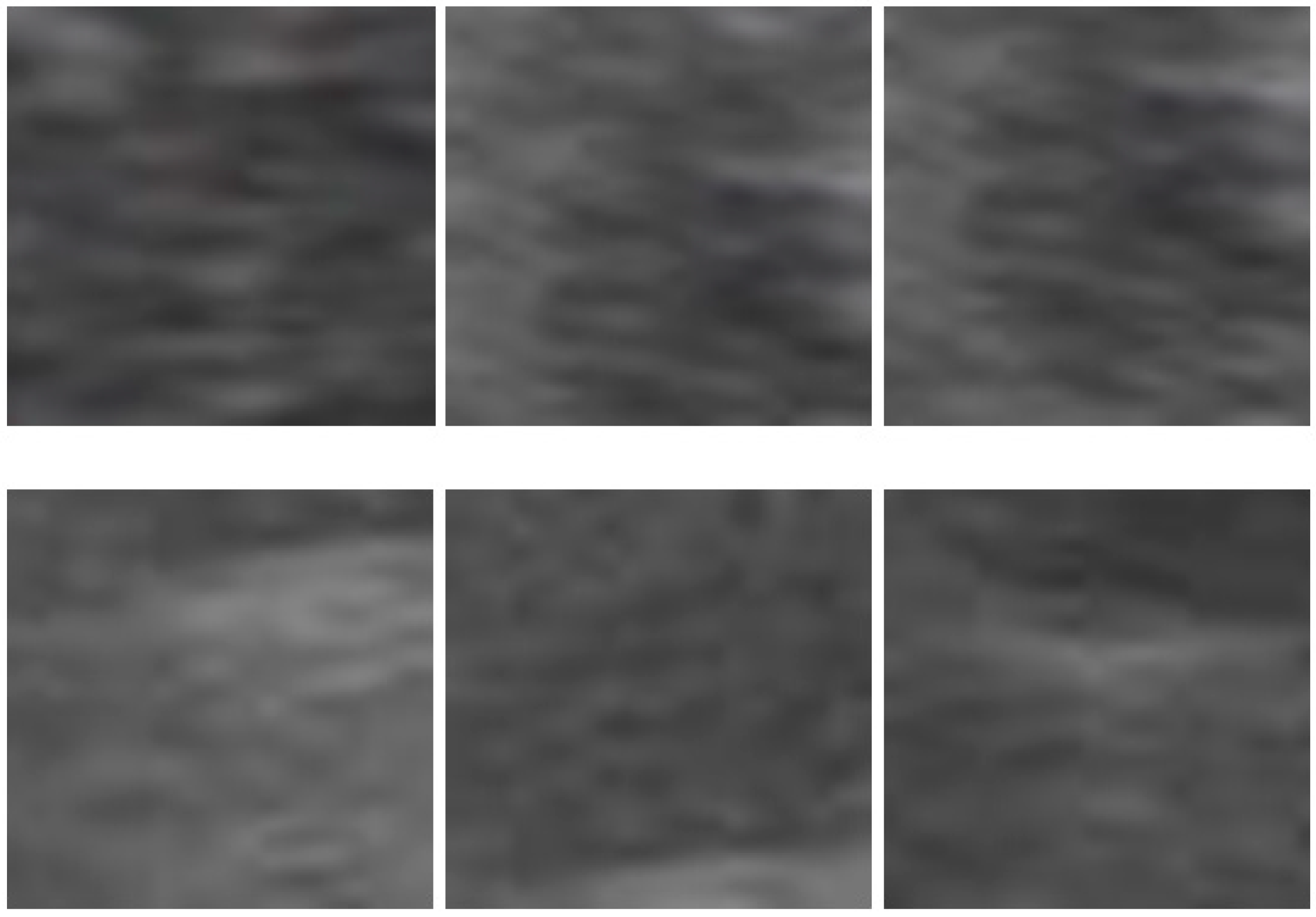
Figure 3.
ROIs taken by MATLAB: The first row shows samples of HCC, and the second row shows samples of liver abscess.
Figure 3.
ROIs taken by MATLAB: The first row shows samples of HCC, and the second row shows samples of liver abscess.

Figure 4.
GLCM process.

Figure 5.
Directions of gray-level co-occurrence matrix.

Figure 6.
Extracting the gray-level co-occurrence matrix (GLCM) from an image.

Figure 7.
Calculation of gray-level co-occurrence matrix.

Figure 8.
GLCM example with .

Figure 9.
GLRLM example. The first row is a 4 × 4 matrix with four gray levels and the others are the corresponding GLRLMs in 4 directions.
Figure 9.
GLRLM example. The first row is a 4 × 4 matrix with four gray levels and the others are the corresponding GLRLMs in 4 directions.

Figure 10.
A 4 × 4 grayscale image and its corresponding GLRLM.

Figure 11.
Results of GLCM features and SVM.

Figure 12.
Results of GLRLM features and SVM.

Figure 13.
Results of all features and SVM.


Table 1.
GLCM features of an image.
| Textural Features | Value | |
|---|---|---|
| 1 | Energy | 0.1386 |
| 2 | Entropy | 2.0915 |
| 3 | Contrast | 0.9960 |
| 4 | Correlation | 0.5119 |
| 5 | Homogeneity | 0.7213 |
| 6 | Sum average | 2.3260 |
| 7 | Sum variance | 2.8829 |
| 8 | Sum entropy | 1.5155 |
| 9 | Difference average | 0.4980 |
| 10 | Difference variance | 0.5542 |
| 11 | Difference entropy | 1.0107 |
| 12 | Information measures of correlation feature 1 | −0.3713 |
| 13 | Information measures of correlation feature 2 | 0.7840 |
Table 2.
GLRLM features of an image.
| Textural Features | Value | |
|---|---|---|
| 1 | SRE | 0.8269 |
| 2 | LRE | 1.6923 |
| 3 | SRHGE | 5.9423 |
| 4 | LRLGE | 0.4348 |
| 5 | LRHGE | 14.3077 |
| 6 | LGRE | 0.3371 |
| 7 | HGRE | 7.6154 |
| 8 | SRLGE | 0.3126 |
| 9 | LRN | 8.3846 |
| 10 | GLN | 3.3077 |
| 11 | RPC | 0.8125 |
Table 3.
Confusion matrix.
| Condition | Positive | Negative | |
|---|---|---|---|
| Prediction | |||
| Positive | True Positive | False Positive | |
| Negative | False Negative | True Negative | |
Table 4.
Accuracy rate without applying selection method.
| GLCM (52 Features) | GLRLM (44 Features) | GLCM + GLRLM (96 Features) |
|---|---|---|
| 75.75% | 54.53% | 61% |
Table 5.
Accuracy rate when applying the sequential forward selection method.
| Without SFS | With SFS | Number of Selected Features | |
|---|---|---|---|
| Accuracy rate with GLCM features | 75.75% | 78% | 5 |
| Accuracy rate with GLRLM features | 54.53% | 88.13% | 7 |
| Accuracy rate with GLCM and GLRLM features | 61% | 89.25% | 9 |
Table 6.
Accuracy rate when applying the sequential backward selection method.
| Without SBS | With SBS | Number of Selected Features | |
|---|---|---|---|
| Accuracy rate with GLCM features | 75.75% | 75.5% | 48 |
| Accuracy rate with GLRLM features | 54.53% | 88.25% | 28 |
| Accuracy rate with GLCM and GLRLM features | 61% | 88.87% | 68 |
Table 7.
F-score of GLCM.
| F | F-Score | F | F-Score | F | F-Score | F | F-Score |
|---|---|---|---|---|---|---|---|
| 1 | 0.094006 | 14 | 0.046439 | 27 | 0.041523 | 40 | 0.048657 |
| 2 | 0.000759 | 15 | 0.003384 | 28 | 0.00427 | 41 | 0.000678 |
| 3 | 0.222294 | 16 | 0.087401 | 29 | 0.104389 | 42 | 0.15354 |
| 4 | 0.166121 | 17 | 0.115392 | 30 | 0.114496 | 43 | 0.128984 |
| 5 | 0.225713 | 18 | 0.092026 | 31 | 0.093941 | 44 | 0.135722 |
| 6 | 0.175996 | 19 | 0.175218 | 32 | 0.176167 | 45 | 0.175231 |
| 7 | 0.129382 | 20 | 0.126291 | 33 | 0.123562 | 46 | 0.118854 |
| 8 | 0.144281 | 21 | 0.098294 | 34 | 0.09322 | 47 | 0.092418 |
| 9 | 0.225882 | 22 | 0.094314 | 35 | 0.100657 | 48 | 0.145838 |
| 10 | 0.219637 | 23 | 0.086611 | 36 | 0.104336 | 49 | 0.149344 |
| 11 | 0.22536 | 24 | 0.096301 | 37 | 0.10026 | 50 | 0.14694 |
| 12 | 0.083251 | 25 | 0.001884 | 38 | 0.00122 | 51 | 0.007818 |
| 13 | 0.000225 | 26 | 0.003192 | 39 | 0.003984 | 52 | 0.000644 |
Table 8.
F-score of GLRLM.
| F | F-Score | F | F-Score | F | F-Score | F | F-Score |
|---|---|---|---|---|---|---|---|
| 53 | 0.309454 | 64 | 0.108676 | 75 | 0.087955 | 86 | 0.135784 |
| 54 | 0.105037 | 65 | 0.026292 | 76 | 0.019915 | 87 | 0.031407 |
| 55 | 0.112888 | 66 | 0.12426 | 77 | 0.136258 | 88 | 0.116255 |
| 56 | 0.258012 | 67 | 0.097652 | 78 | 0.092349 | 89 | 0.140583 |
| 57 | 2.50 × 10⁻⁵ | 68 | 1.20 × 10⁻⁵ | 79 | 4.00 × 10⁻⁶ | 90 | 1.20 × 10⁻⁶ |
| 58 | 0.113405 | 69 | 0.111519 | 80 | 0.110956 | 91 | 0.110342 |
| 59 | 0.187865 | 70 | 0.183068 | 81 | 0.17762 | 92 | 0.175827 |
| 60 | 0.064373 | 71 | 0.108361 | 82 | 0.109202 | 93 | 0.107328 |
| 61 | 0.11555 | 72 | 0.053881 | 83 | 0.062097 | 94 | 0.083418 |
| 62 | 0.503327 | 73 | 0.297173 | 84 | 0.266923 | 95 | 0.271874 |
| 63 | 0.009315 | 74 | 0.001695 | 85 | 0.003806 | 96 | 0.002537 |
Table 9.
Comparison between searching all and using a threshold.
| Threshold | Search All | |
|---|---|---|
| GLCM | 76.25% | 77.25% |
| GLRLM | 87.125% | 87.125% |
| GLCM + GLRLM | 87.375% | 88.875% |
Table 10.
Overall results.
| No Feature Selection | SFS | SBS | F-Score (Threshold) | F-Score (Search All) | |
|---|---|---|---|---|---|
| GLCM + SVM | 75.75% | 78% | 75.5% | 76.25% | 77.25% |
| GLRLM + SVM | 54.53% | 88.13% | 88.25% | 87.125% | 87.125% |
| All features + SVM | 61% | 89.25% | 88.87% | 87.375% | 88.875% |
© 2019 by the authors. Licensee MDPI, Basel, Switzerland. This article is an open access article distributed under the terms and conditions of the Creative Commons Attribution (CC BY) license (http://creativecommons.org/licenses/by/4.0/).
Share and Cite
MDPI and ACS Style
Xu, S.S.-D.; Chang, C.-C.; Su, C.-T.; Phu, P.Q. Classification of Liver Diseases Based on Ultrasound Image Texture Features. Appl. Sci. 2019, 9, 342. https://0-doi-org.brum.beds.ac.uk/10.3390/app9020342
AMA Style
Xu SS-D, Chang C-C, Su C-T, Phu PQ. Classification of Liver Diseases Based on Ultrasound Image Texture Features. Applied Sciences. 2019; 9(2):342. https://0-doi-org.brum.beds.ac.uk/10.3390/app9020342
Chicago/Turabian StyleXu, Sendren Sheng-Dong, Chun-Chao Chang, Chien-Tien Su, and Pham Quoc Phu. 2019. "Classification of Liver Diseases Based on Ultrasound Image Texture Features" Applied Sciences 9, no. 2: 342. https://0-doi-org.brum.beds.ac.uk/10.3390/app9020342
Note that from the first issue of 2016, this journal uses article numbers instead of page numbers. See further details here.