Modeling Implicit Trust in Matrix Factorization-Based Collaborative Filtering

Abstract

Recommendation systems often use side information to both alleviate problems, such as the cold start problem and data sparsity, and increase prediction accuracy. One such piece of side information, which has been widely investigated in addressing such challenges, is trust. However, the difficulty in obtaining explicit relationship data has led researchers to infer trust values from other means such as the user-to-item relationship. This paper proposes a model to improve prediction accuracy by applying the trust relationship between the user and item ratings. Two approaches to implement trust into prediction are proposed: One involves the use of estimated trust, and the other involves the initial trust. The efficiency of the proposed method is verified by comparing the obtained results with four well-known methods, including the state-of-the-art deep learning-based method of neural graph collaborative filtering (NGCF). The experimental results demonstrate that the proposed method performs significantly better than the NGCF, and the three other matrix factorization methods, namely, the singular value decomposition (SVD), SVD++, and the social matrix factorization (SocialMF).

1. Introduction

Recommendation systems help users overcome the problem of information overload by providing personalized recommendations. One of the most common methods for generating recommendations is collaborative filtering (CF), in which predictions are made using a user’s past behavior [1]. The concept behind CF is that users with similar behaviors interact with the same items, and tend to provide similar ratings.

CF can be broadly categorized into memory-based methods, in which the entire rating history is used to determine the relationship among users or items, and model-based methods, in which a model is constructed using the users’ rating matrix. The simplest form of memory-based CF involves calculating the similarity between users and making predictions using the similarity of the k-nearest neighbors. Although similarity-based methods are simple, they suffer several limitations including the cold start problem, in which not enough user ratings are available for prediction, data sparsity, and scalability. Accordingly, calculating trust has been widely used as an alternative to calculating similarity in CF [2,3,4]. Due to the scalability issues associated with memory-based methods, many large-scale systems in industrial settings use model-based methods to provide recommendations [5,6].

The most popular model-based method is matrix factorization (MF) and its variations [6]. In this method, the algorithm is optimized to determine two low-rank matrices containing the latent features of the items and users; these matrices are then combined to obtain the original matrix [6]. A regularization factor is used to prevent overfitting. The singular value decomposition (SVD) is imposed as a baseline for model-based CF. However, MF models are difficult to generalize to the data when the original rating matrix is sparse. Several approaches have been proposed to address this challenge.

The simplest and most common approach to resolve the sparsity problem involves inputting artificial data into the original matrix, and mean ratings are often used for this purpose. To address the problems associated with data sparsity in low-rank matrix approximation, Sebrero and Jaakkola [7] proposed a model that uses a weight inversely proportional to the noise variance. Similarly, Lee et al. [8] proposed an approach, namely, local low-rank matrix approximation (LLORMA), which approximates the observed matrix as the weighted sum of local low-rank matrices that are targeted to the local regions of the observed matrix. To construct the final approximated matrix, several local models are aggregated. Mackey et al. [9] proposed a similar method referred to as divide-and-conquer (DFC) MF. In contrast to LLORMA, DFC uses overlapping partitions of the observed matrix to construct the local models.

To improve the efficiency of recommendation systems, the use of side information has been widely researched. Apart from side information such as the context and user and item characteristics, trust is often used as a reliable measure to incorporate into the CF technique. However, obtaining the explicit trust link between users is difficult. Here, we propose a new trust measure that can be derived directly from the user’s preference matrix. In contrast to most trust metrics, which measure the degree of reliability between two users, our proposed metrics measure the user’s trust regarding the preference they have expressed. The metric consists of two components: (1) the user’s proportional rating on the target item, and (2) item popularity. Then, the resulting trust metric is incorporated into predictions. We used two approaches to do so; one involves an estimation of the trust matrix from the initial trust values, and the second directly adds trust values into the prediction.

CF models that perform optimization based on the prediction accuracy can be viewed as regression problems. The method proposed in the present work is likewise modeled as a regression problem. One of the most common evaluation metrics used for calculating the prediction accuracy in recommendation systems is the mean absolute error (MAE), which is based on the prediction error; in particular, the MAE indicates the mean absolute difference between the predicted value and the actual rating. Our proposed method adopts a new trust inference mechanism and incorporates trust as side information into MF models to make better predictions. Therefore, we use the prediction accuracy using MAE as a measure for evaluating the proposed model.

The main contributions of this study can be summarized as follows: (1) a new trust inference model is proposed for implicit data; (2) the trust model is incorporated in MF methods; and (3) the model is empirically evaluated using real-world data sets.

The remaining paper is organized as follows. In Section 2, we review related works. Section 3 describes the model formulation, including that of models pertaining to the MF, SVD, trust, and the combined model. Section 4 describes the experimental setup, and the results are discussed in detail in Section 5. Section 6 provides a discussion of the implications of the model, and Section 7 presents the conclusions.

2. Related Work

In this section, we discuss some related work on recommendation systems that use the trust relationship to improve accuracy.

Massa and Avesanin [10] reported on one of the earliest attempts to use trust in a recommender system. Inspired by the PageRank algorithm [10], the authors used trust propagation in the network to estimate the trust matrix. However, a drawback of this model was that it combined the similarity matrix with the trust matrix, thereby increasing the computational time and dependence on the similarity matrix.

Golbeck [11] designed a model for movie recommendation, named TidalTrust, which uses social trust, i.e., trust inferred from a social network. The concept behind this model is that people prefer recommendations from acquaintances or friends instead of from relatively unknown people. Trust is defined as one’s commitment to act in the future, in such a way that leads to a positive outcome for the one who relies on the committed action; it is calculated using a modified version of the breadth-first search. In the prediction phase, the calculated trust is used to weight the ratings of the neighbors.

In [12], O’Donovan proposed a trust model, in which trust is inferred as the target user’s contribution to the prediction accuracy. In contrast to all the other models discussed in this section, this model does not depend on explicit social links to infer trust. However, this model has considerably higher computation costs because of the initial prediction calculation during the trust matrix generation. Addressing these issues with prediction accuracy-based trust models, Zahir et al. [13] proposed AgreeRelTrust, which is a model that uses the agreement between users to infer trust, eliminating the need to calculate the initial predictions. This method also takes into account the activeness of the users when calculating the trust; however, the method is a memory-based model, and is thus not as computationally efficient as the MF variants.

Ma et al. [14] used an SVD sign-based community mining method to discover trust and distrust to improve the accuracy of the CF-based recommendation system. The users in the system are first clustered into k communities. The rationale behind clustering users is that users within the same community tend to share a positive relationship, whereas a negative relationship exists between different communities. Although the method improves the accuracy of the recommendations, the trust mining method uses a binary trust value to indicate trust and distrust. Owing to the binary nature of the implicit rating, most trust-based recommenders that rely on the Pearson similarity fail. SVD++, an extension of SVD, takes auxiliary information such as the users’ historical consumption [15] and combines the neighborhood method with MF. However, the model is limited to user-side implicit feedback, ignoring the item side, and treats all implicit feedback equally.

Another line of research that has recently gained popularity is graph-based recommendation, in which the model relies on a bipartite graph generated from user interactions. In a recent work, Niu et al. [16] proposed graph-based collaborative filtering (GCF), addressing the issues imposed by SVD++. The recommendation process is modeled as a bipartite graph structure, considering both item-side and user-side implicit feedback. Latapy et al. [17] proposed a general graph-based framework for top-N recommendations (GraFC2T2) that accounts for several side information aspects, including trust. First, the graph structure is constructed from the data, and is then used to make recommendations. The graph structure captures both the content-based features and edge weight time. The PageRank algorithm [18] runs on the graph to make recommendations, and the final recommendations are updated based on the trust between user pairs. This trust integration uses both explicit and implicit trust. The key advantage of GraFC2T2 is that it is a highly modular framework. In contrast, in the method proposed by Papagelis et al. [19], trust is obtained using the Jacobian similarity between two users.

State-of-the-art recommendation systems are heavily dependent on deep learning. In [20], Hinton et al. used a two-layered graphical model named restricted Boltzmann machines (RBM) as one of the earliest methods that use deep learning in CF. To avoid the high computation cost of the maximum likelihood method, the model uses constructive divergence (CD) as the objective function. Since then, many deep learning-based CF methods have emerged. For a detailed survey of state-of-the-art deep learning recommendation systems, interested readers are referred to [21]. In a very recent work, arguing the limited representation of collaborative signals in embeddings in deep learning models, Wang et al. [22] proposed neural graph collaborative filtering (NGCF), in which the item embedding and user embedding are fed into two separated neural network layers. The inner product of the final outputs from the two networks are used to estimate a user’s preference to the target item. The network learns the graph structure of the high-order connectivity between the items and the user. In the present work, this method is used as one of the baselines.

Social Trust Ensemble (STE) is a model-based method proposed by Ma et al. [23], in which the latent features of the target users’ neighbors’ ratings are used to model trust. This method combines matrix factorization and trust-based recommendation. Addressing the issue of trust propagation in STE, Jamali et al. [24] proposed social matrix factorization (SocialMF), which is a matrix factorization method that employs the trust link between users to increase prediction accuracy. Addressing the cold-start problem in MF methods, Forsati et al. [25] proposed a MF method that uses explicit trust and distrust. Similar to the STE and GraFC2T2 methods, this method uses explicit trust links. However, obtaining a trust link between users is difficult, and very few public data sets contain trust relationships. For this reason, they adapted the Pearson correlation coefficient (PCC) as a trust metric for their experimental data set. Among other issues, PCC-based trust metrics fail on binary data. Therefore, in this work, we propose a new trust inference mechanism for MF models that use binary data.

3. Model

This section describes the model formulation. As the core of the model is MF, MF is described in the first subsection. Next, the SVD is described, which is followed by the description of the trust model; finally, we propose the combined model. Please note that the terms rating and preference are used interchangeably in this paper.

3.1. Matrix Factorization

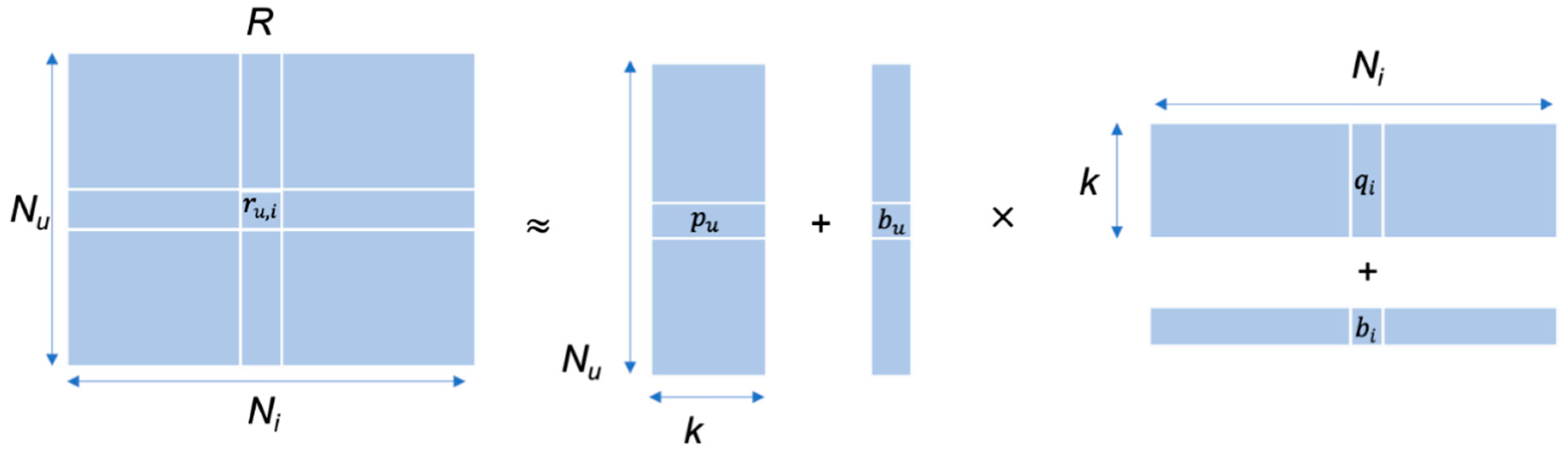
The goal of MF is to determine two $k$ dimensional latent vectors $p_u\mathrm{and}{q}_i\in {\mathbb{R}}^K$ that represent user $u\in \left\{1,2,3\dots N_u\right\}$ and item $i\in \left\{1,2,3\dots N_i\right\}$, respectively. The inner products of both the latent vectors approximate the original rating matrix $R_{N_u\times N_i}$. The predictions are calculated as follows:

$$\widehat{r_{u,i}}=f\left(\langle p_u,q_i\rangle +b_u+b_i\right),$$

(1)

where $\langle p_u,q_{\mathrm{i}}\rangle$ is the inner product of both the latent vectors; $b_u$ and $b_i$ denote the user and item bias, respectively; and $\widehat{r_{u,i}}$ is the predicted item rating of item $i$ to user $u$. This aspect is shown in Figure 1, in which $r_{u,i}$ is a part of the original rating matrix $R$.

3.2. SVD++

SVD++ is the most widely used latent factor model for MF because of its superior prediction accuracy. In SVD++, two vectors $p_u$ and $q_i$, which respectively contain the latent features of the users and items, are learned by minimizing the regularized mean squared error on the set of known ratings:

$$min{{\displaystyle \sum }}_{u,iϵR}{\left(r_{u,i}-\mu -b_u-b_i-q_i^T\left(p_u+{\left|I_u\right|}^{-\frac{1}{2}}{\displaystyle \sum }_{jϵI_u}{y}_j\right)\right)}^2+\lambda ({\parallel q_i\parallel }^2+{\parallel p_u\parallel }^2+{\displaystyle \sum }_{jϵI_u}{\parallel y_j\parallel }^2+b_u^2+b_i^2)$$

(2)

where $R$ contains user–item $\left(u,i\right)$ pairs for which rating $r_{u,i}$ is known; $\mu$ is the mean rating, $I_u$ is user u’s item vector, $y_j$ is the $j$th rating in $I$, and $\lambda$ is the regularization constant. In contrast to the regular MF model defined in Equation (1), SVD++ takes the perspective of implicit feedback.

Then, the predictions are made using the learned latent features:

$$\widehat{r_{u,i}}=\mu +b_u+b_i+q_i^T\left(p_u+{\left|I_u\right|}^{-\frac{1}{2}}{\displaystyle \sum }_{jϵI_u}{y}_j\right),$$

(3)

where ${\left|I_u\right|}^{-\frac{1}{2}}{\displaystyle \sum }_{jϵI_u}{y}_j$ captures the user’s implicit feedback.

3.3. Trust Model

3.3.1. Binary Conversion

User $u$’s preference for item $i$ is represented using the binary variable ${\dot{r}}_{u,i}$. The binary value is defined as:

$${\dot{r}}_{u,i}=\{\begin{array}{c}1s>\beta \\ 0s\le \beta \end{array}$$

(4)

where $s$ is the preference, and $\beta$ is the threshold value. In cases in which the user preference is defined as the number of page views/site visits/interactions, $\beta$ is 0. Furthermore, the binary value ${\dot{r}}_{u,i}$ is one if the user has interacted with the item; otherwise, its value is 0. By using this criterion, we can generate the new binary preference matrix even if the data are explicit. If the data include explicit ratings, a suitable value for $\beta$ is the midpoint of the rating scale. One notable advantage of this strategy is that this representation can take various types of implicit data such as the number of views, site visits, and time spent on the site. The binary conversion steps defined in Equation (4) are not necessary if the data is already in the binary format (e.g., liked or not liked), as these may add unnecessary computation to the algorithm. Although Equation (4) supports the generation of a binary preference for different types of implicit data, it takes only a single input. However, in the real-world setup, it is common to use as many available implicit feedbacks as possible. The additional implicit data can be incorporated into Equation (4) using a weighting mechanism as follows:

$$F={\displaystyle \sum }_0^m{s}_m{w}_m$$

(5)

$$TF=\frac{F}{1+F}$$

(6)

where F is the weighted sum of the total feedbacks, $s$ is the implicit feedback of the $m$th type, $w$ is the respective weight, and TF is the resulting combined feedback. We use Equation (6) to ensure that the total weighted feedback lies in the range between 0 and 1. This formulation accommodates both the explicit rating and multiple forms of implicit rating. To binarize the data, we then change Equation (4) as follows:

$${\dot{r}}_{u,i}=\{\begin{array}{c}1TF>\beta \\ 0TF\le \beta \end{array}$$

(7)

where $\beta$ is the threshold and can be set to a preferred value, which is usually 0.5. In contrast to Equation (4), this formulation handles multiple inputs; therefore, the output binary value represents a richer form of preference.

3.3.2. Initial Trust Inference

We define trust as the degree of a user’s confidence toward the item preference they have expressed. It is common for users to rate items without having full confidence. For example, consider a case in which a user is asked to rate a popular movie and an average movie. The user liked both movies, but not equally. Nevertheless, the user provides a rating of 5 stars for both of the movies. In this case, it is highly likely for the user to have a higher confidence in the rating expressed for the popular movie than that for the average movie. Similarly, because of experience, a user who watches more movies would have a higher degree of confidence in their rating than a user who watches fewer movies. Conversely, this measure can be seen as the amount of user trust pertaining to a recommendation made by the recommendation system. This value is calculated as the product of the user’s proportional rating and item popularity:

$$prop\_rating=\frac{\left|I_u\right|}{N_u}$$

(8)

$$item\_popularity=\frac{\left|U_i\right|}{N_i}$$

(9)

$$t_{u,i}=prop\_rating\times item\_popularity$$

(10)

where $t_{u,i}$ is user $u$’s trust toward item $i$’s preference that he/she has expressed, $\left|I_u\right|$ is the length of the user’s preference vector, $\left|U_i\right|$ is the item’s preference vector, and $N_i$ and $N_u$ denote the total number of items and users in the set, respectively. The values for $prop\_rating$ for a specific user are the same for all the entries. Similarly, the values of $item\_popularity$ are the same for any specific item, as seen in lines 10–13 of Algorithm 1, which describes the initial trust calculation. Consequently, some computations are eliminated when calculating the trust. Another advantage of this trust measure is that it can also be applied to explicit preferences.

Algorithm 1 Pseudocode for initial trust calculation.

1: procedure $\mathrm{GenerateInitialTrust}(RatingMatrix,\beta ,w)$

2:  $n\_users=length\left(RatingMatrix.rows\right)$$,n\_items=length\left(RatingMatrix.cols\right)$

3:  $T=zeros\left(n\_users,n\_items,\right)$

4:  $R=generateBinaryMatrix\left(RatingMatrix,\beta ,w\right)$, //generating binary matrix

5:   for $u=0,u++,u<n\_users$ do

6:    $I_u=R\left(u,:\right)$,

7:     $Prop\_rating\leftarrow length\left(I_u\right)/n\_users$

8:     $Item\_popularity=0$

9:    for $i=0,i++,i<n\_items$ do

10:      if $i==0$ then

11:        $U_i=R\left(:,i\right)$,

12:        $Item\_popularity\leftarrow length\left(U_i\right)/n\_item$

13:      end if

14:      $T\left(u,i\right)=Prop\_rating\times Item\_popularity$

15:    end for

16:   end for

17:  return $T$

18: end procedure

The function generateBinaryMatrix in line 4 of Algorithm 1 converts the preference matrix into a binary matrix by looping through the entries and comparing the values with $\beta$. If the preference matrix consists of multiple dimensions, before the comparison, the matrix is flattened using Equations (5) and (6).

Please note that unlike most trust models [4,11], this trust measure considers the relationship between only the user and the user’s expressed preference. However, the term “trust” in most of the trust models refers to a relationship either between a user and another user or between an item and another item. Therefore, the configuration of the resulting trust matrix has the same shape as that of the rating matrix.

Since our objective is to improve the prediction accuracy by incorporating the trust values, we propose two approaches involving use of the estimated trust and use of the initial trust. The first approach involves estimation of the trust values before incorporating it into the predictions. In contrast, the second approach uses only the initially calculated trust values.

3.4. Approach 1: Use Estimated Trust

One of the simplest ways to incorporate trust into the preference calculation is to aggregate both the trust matrix and predicted preference matrix into one matrix. However, the trust matrix is very sparse, as it is derived from a sparse original preference matrix. Consequently, the trust values can only be aggregated with non-empty entries in the original preference matrix. This problem can be solved by learning the latent factors of trust, and then aggregating them with the latent factors of the preference matrix. To this end, the trust matrix is factorized into two low-dimensional trust vectors, $t{p}_u$ and $t{q}_i$, which are associated with the users and items, respectively. Similar to the SVD, we determine $t{p}_u$ and $t{q}_i$ by minimizing the estimation error as:

$$min{{\displaystyle \sum }}_{u,iϵR}{\left(t_{u,i}-t{q}_i^{T}t{p}_u\right)}^2+\lambda$$

(11)

where $t{q}_i^{T}t{p}_u$ is the inner product of the two trust vectors, and $\lambda$ is the regularization constant, which prevents overfitting of the model to the training data.

As previously mentioned, $p_u$ and $q_i$ capture the general latent features of both the users and items. Similarly, the trust-related features are captured via $t{p}_u$ and $t{q}_i$. The primary goal of combining the general latent features with the trust features is to obtain two final latent vectors to create a model that can capture the best aspects of the trust-related and general hidden features. As the latent vectors can be combined in several ways, we tested the following three combination methods:

• Subtract trust
  In this method, the two final trust latent vectors are derived by deducting the trust latent vectors from $p_u$ and $q_i$ as follows:

  $$p{u}_{final}=p_u-t{p}_u,$$

  (12)

  $$q{i}_{final}=q_i-t{q}_i,$$

  (13)

  where $p{u}_{final}$ and $q{i}_{final}$ are the final user and item latent vectors, respectively. Intuitively, this operation can be viewed as adding the trust as a type of bias to the latent features. The same results can be achieved even if the trust vectors are concatenated with $p_u$ and $q_i$. However, this operation would change the length of the final vectors, and therefore, the dimensions of the vectors in the prediction formula must be adjusted accordingly.
• Weight by trust
  In this method, weight latent preference vectors are determined with the latent trust vector as follows:

  $$p{u}_{final}=p_u\times t{p}_u;$$

  (14)

  $$q{i}_{final}=q_i\times t{q}_i.$$

  (15)
  Similar to the method of adding the vectors, this method does not change the length of the final vectors.
• Add mean trust
  Unlike the previous two methods, in this method, the length of the two final vectors are different. Therefore, the user-implicit feedback vector in the final prediction needs to be padded with a zero. The final two latent vectors are derived as follows:

  $$p{u}_{final}=concat\left(p_u+mean\left(t{p}_u\right)\right)$$

  (16)

  $$q{i}_{final}=concat\left(q_i+mean\left(t{q}_i\right)\right)$$

  (17)

For the three above-mentioned methods, the final predictions can be made using the following equation:

$$\widehat{r_{u,i}}=\mu +b_u+b_i+q{i}_{final}^T\left(p{u}_{final}+{\left|I_u\right|}^{-\frac{1}{2}}{\displaystyle \sum }_{jϵI_u}{y}_j\right),$$

where $q{i}_{final}^T$ and $p{u}_{final}$ are the combined trust and latent vectors of the items and users, respectively. The remaining parameters are the same as those in the SVD++, as defined in Equation (3).

The concept behind the combination of the trust and feature matrices is that each entry in the approximated matrix also accounts for the trust degree. It is trivial to use the same algorithm with different inputs (i.e., trust for trust features and ratings for the item and user features). However, reusing the same algorithm twice increases the computational cost by two times. Since the extraction of the latent features for both the trust model and the SVD model are similar, they can be combined into one, as presented in Algorithm 2, which illustrates the latent vector approximation. As shown in lines 10–14 of Algorithm 2, the stochastic gradient descent (SGD) is used to estimate the model parameters $Pu,Qi,TPu,\mathrm{and}TQi$.

Algorithm 2 Pseudocode for latent vector approximation.

1: procedure $\mathrm{GenerateLatentModel}(RatingMatrix,InitialTrustMatrix,\alpha ,\lambda ,n\_epoch$)

2:   $n\_users=length\left(RatingMatrix.row\right)$$,n\_items=length\left(RatingMatrix.row\right)$

3:   $Pu,Qi=Initalize\left(n\_users,n\_items,k\right)$

4:   $TPu,TQi=Initalize\left(n\_users,n\_items,k\right)$

5:   for $n=0,n++,n<n\_epoch$ do

6:    for $u=0,u++,u<n\_users$ do

7:     for $i=0,i++,i<n\_items$ do

8:      $p_u=Pu\left(u\right),q_i=Qi\left(i\right),t{p}_u=TPu\left(u\right),t{q}_i=TQi\left(i\right),r_{u,i}=RatingMatrix\left(u,i\right)$

9:      $I_u=RatingMatrix\left(u,:\right)$$,U_i=RatingMatrix\left(:,i\right)$

10:        $\mu =mean\left(RatingMatrix\right)$$,b_i=\mu -mean\left(U_i\right)$

11:        $b_u=\mu -mean\left(I_u\right)$, $t_{u,i}=InitialTrustMatrix\left(u,i\right)$

12:        $ImpFactor=sqr\left(len\left(I_u\right)\right)\times sum\left(I_u\right)$

13:        $reg=\lambda (len{\left(I_u\right)}^2+len{\left(U_i\right)}^2+$ ${b_u}^2+{b_i}^2)$

14:        $\delta q=-q_i\times \left(r_{u,i}-\mu -b_i-b_u-p_u.q_i-reg\right)$

15:        $\delta p=-p_u\times \left(r_{u,i}-\mu -b_i-b_u-(p_u+ImpFactor\right).q_i-reg)$

16:        $q_i\leftarrow q_i+\alpha \times \delta q$

17:        $p_u\leftarrow p_u+\alpha \times \delta p$

18:         //trust estimation

19:        $\delta tq=-t{q}_i\times \left(t_{u,i}-t{p}_u.t{q}_i-\lambda \right)$

20:        $\delta tp=-t{p}_u\times \left(t_{u,i}-t{p}_u.t{q}_i-\lambda \right)$

21:        $t{q}_i\leftarrow t{q}_i+\alpha \times \delta tq$

22:        $t{p}_u\leftarrow t{p}_u+\alpha \times \delta tp$

23:        $Pu\left(u\right)=p_u,Qi\left(i\right)=q_i,TPu\left(u\right)=t{p}_u,TQi\left(i\right)=t{q}_i$

24:      end for

25:     end for

26:   end for

27:   return $Pu,Qi,TPu,TQi$

28: end procedure

Since both the trust and latent features are estimated together, they are trained with the same number of epochs. Then, the outputs of Algorithm 1 are combined using any of the three combination methods mentioned earlier.

3.5. Approach 2: Use Initial Trust

In this approach, the trust values are calculated on the fly only in the prediction stage. The model learns $p_u$ and $q_i$ by minimizing the SVD++, as defined in Equation (2). Then, the trust value is aggregated into the trust as follows:

$$\widehat{t{r}_{u,i}}=\{\begin{array}{c}\widehat{r_{u,i}}\times t_{u,i},if{t}_{u,i}\ge {\mu }_t\\ \widehat{r_{u,i}}+t_{u,i},if{t}_{u,i}<{\mu }_t\end{array},$$

(18)

$$\widehat{f{r}_{u,i}}=\widehat{r_{u,i}}+\widehat{t{r}_{u,i}},$$

(19)

where $t_{u,i}$ is the trust calculated using Equation (10), ${\mu }_t$ is the mean trust of the data set, $\widehat{r_{u,i}}$ is the predicted rating obtained using Equation (3), and $\widehat{f{r}_{u,i}}$ is the final predicted rating for user $u$’s item $i$. The clear advantage of this approach is that it does not involve performing the trust calculation at the training stage.

4. Experiment Details

4.1. Data Set

We validate the efficacy of our model using three MovieLens (GroupLens, University of Minnesota, Minneapolis, USA) data sets: ML-1m, ML-100k, and a 100k subset of the ML-20m data set [26].

The ML-1m data set contains 1 million ratings collected from 4000 users on 6000 items, released in February 2003. The ML-100k data set contains 100,000 ratings of 1700 items by 1000 users, released in April 1998; this is one of the most widely used data sets in recommendation system research, especially for implicit trust-based recommendation systems [2,4,25]. The ML-20m subset contains 100,000 ratings of 696 users for 7691 movies. For convenience, we have first chosen 100,000 ratings from the ML-20m data set to include in the subset. Since the proposed methods are dependent on the number of the users and items, we have chosen data sets with varying lengths to see how they perform under different lengths.

The ratings are scaled from 1 to 5. For the experiment, we modeled a data entry as a tuple containing the user ID, item ID, and ratings. We performed five-fold cross-validation on each test methods for all the data sets.

Since these data sets contain only explicit non-binary ratings and no implicit data, for the binarization, we employed Equation (2) with $\beta =2.5$ (midpoint of the rating scales).

4.2. Comparison Models

In the performed experiments, the following models were compared:

• SVD model: The latent vectors represent the user and items, and their inner product is used to generate the estimated ratings.
• SVD++ model: An extension of SVD, which considers the implicit feedback.
• NGCF model: A state-of-the-art graph-based collaborative filtering model, which explores higher-order connectivity in the user–item graph by using deep learning techniques.
• Subtract-trust (S-Trust) model: As discussed in Section 3.4, in this model, the latent item vectors and latent user vectors are added to the trust latent vectors. The predictions are made in a manner similar to that used in the SVD++.
• Weighted-trust (W-Trust) model: This method is similar to the S-trust, except that the latent vectors are multiplied instead of added.
• Mean-trust concatenation (M-Trust) model: This method is also similar to the S-Trust and W-Trust models; however, instead of adding or multiplying the trust vectors, the mean values of the latent trust vectors are added to the item and user latent vectors.
• Initial trust (I-Trust) model: This method does not calculate the latent vectors for trust (see Section 3.5). Instead, it incorporates the initial trust directly into the predictions in the prediction calculation stage.
• SocialMF model: This is a well-known MF method that uses trust to increase the prediction accuracy.

The first three methods are the baselines, and the last four methods are the proposed test methods.

4.3. Evaluation Metrics

As mentioned in the Introduction, the model is formulated as a rating regression problem. Additionally, in the industry, prediction accuracy is often measured using a method that uses prediction error. Therefore, we use the MAE to evaluate our models. The MAE measures the deviation of the predicted values from the actual value for all predictions, and is calculated as follows:

$$\mathrm{MAE}=\frac{{{\displaystyle \sum }}_{u,i}\left|\widehat{f{r}_{u,i}}-{\dot{r}}_{u,i}\right|}{n}$$

(20)

where $n$ is the number of predications made, ${\dot{r}}_{u,i}$ is the actual binary rating, and $\widehat{f{r}_{u,i}}$ is the predicted rating.

4.4. Experimental Setup

We implemented all the models using the Surprise framework, which is a python-based recommendation framework developed by Hug [27] that is widely used for research as well as practical implementation. The experiments were conducted on a Dell PowerEdge T630 server (Dell Inc., Round Rock, TX, USA) with 2.1 Hz 32 cores and 64 GB RAM. For reproducibility, the code for the experiment is shared on GitHub (see the Supplementary Materials). We slightly modified the NGCF code provided by the original developers [21] to cater to our evaluation metric and data sets.

The details of the parameters used in the experiment are presented in

Table 1. Model parameters for the experimental methods. I-Trust: Initial trust, M-Trust: mean-trust concatenation, NGCF: Neural graph collaborative filtering, S-trust: Subtract-trust, SocialMF: Social matrix factorization, SVD: Singular value decomposition, SVD++: An extension of SVD that considers the implicit feedback, W-Trust: Weight-trust.

Method	k	Learning Rate	Reg	Epochs
SVD	20	0.005	0.02	20
SVD++	20	0.005	0.02	20
S-Trust	20	0.005	0.02	20
W-Trust	20	0.005	0.02	20
M-Trust	20	0.005	0.02	20
I-Trust	20	0.005	0.02	20
NGCF	-	1 × 10−5	0.001	400
SocialMF	-	-	-	10

NCGF and SocialMF parameters are adopted from the authors’ respective papers [21,24].

. For simplicity, we use the suggested default parameters in the Surprise framework.

SocialMF requires binary trust links between users. However, the data sets do not contain relationship links between users. For simplicity, we have generated the trust links using the following strategy: If two users have commonly rated a movie, we have created a link between them. Otherwise, they share no trust link.

5. Results

In this section, we present the results of the several experiments for each of the data sets.

5.1. ML-100k

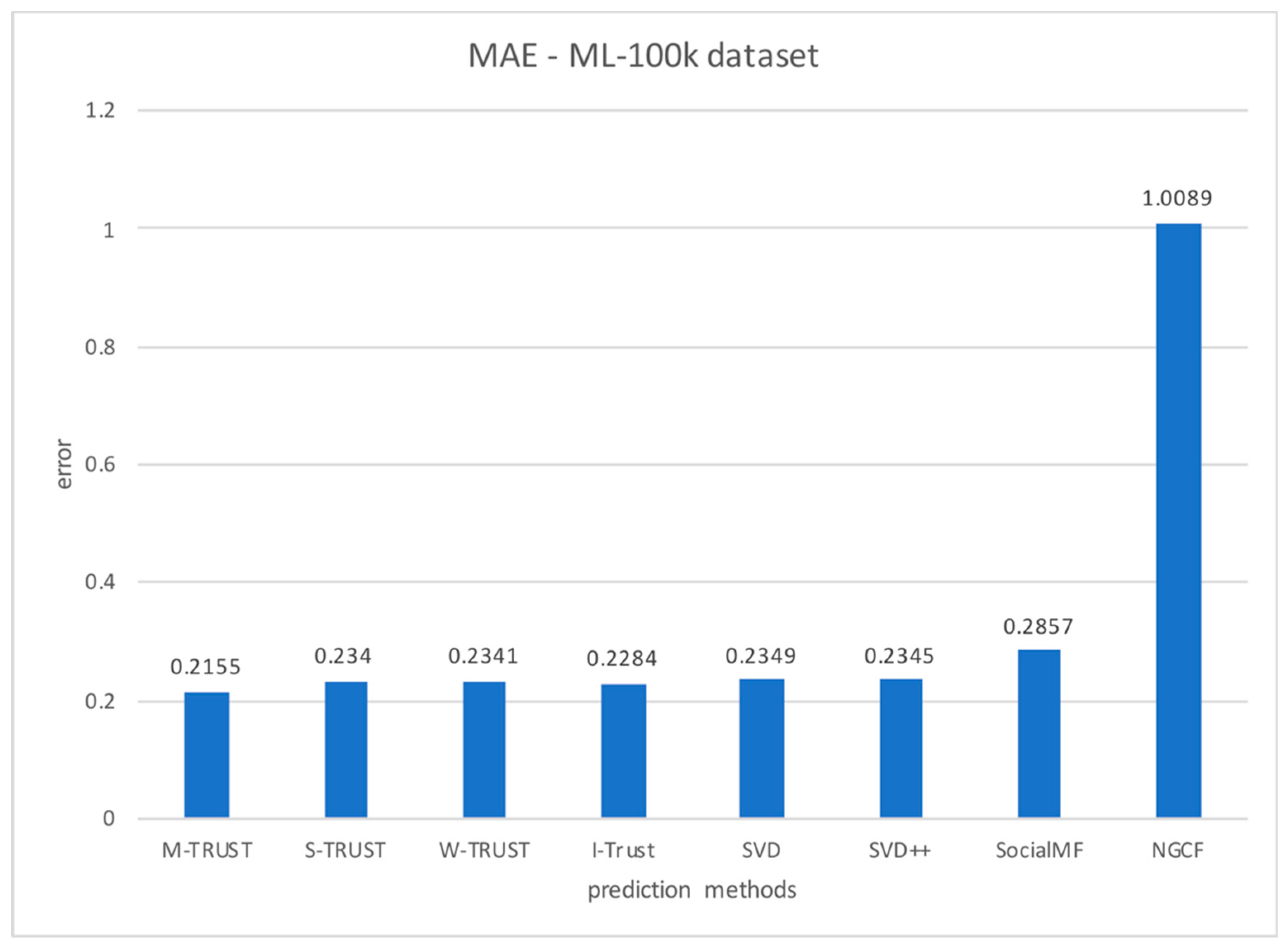
Figure 2 shows the results for the ML-100k data set. All of the trust-based methods provide a better prediction accuracy than those of the baseline methods on the ML-100k data set. NGCF demonstrates the worst performance, whereas the M-Trust model demonstrated the best performance, with significant performance improvements of 9%, 8.82%, 32.58%, and 368.17% compared to SVD, SVD++, SocialMF, and NGCF, respectively. The performance of S-Trust was slightly better than that of W-Trust; it demonstrated a performance improvement of 0.38%, 0.21%, 22.1%, and 331.15%, against SVD, SVD++, SocialMF, and NGCF, respectively. The corresponding improvement values for the W-Trust were 0.34%, 0.17%, 22%, and 330.97%, respectively. I-Trust demonstrated the second-best performance, with performance improvements of 2.85%, 2.67%, 25.09%, and 341.72% compared to the baseline methods.

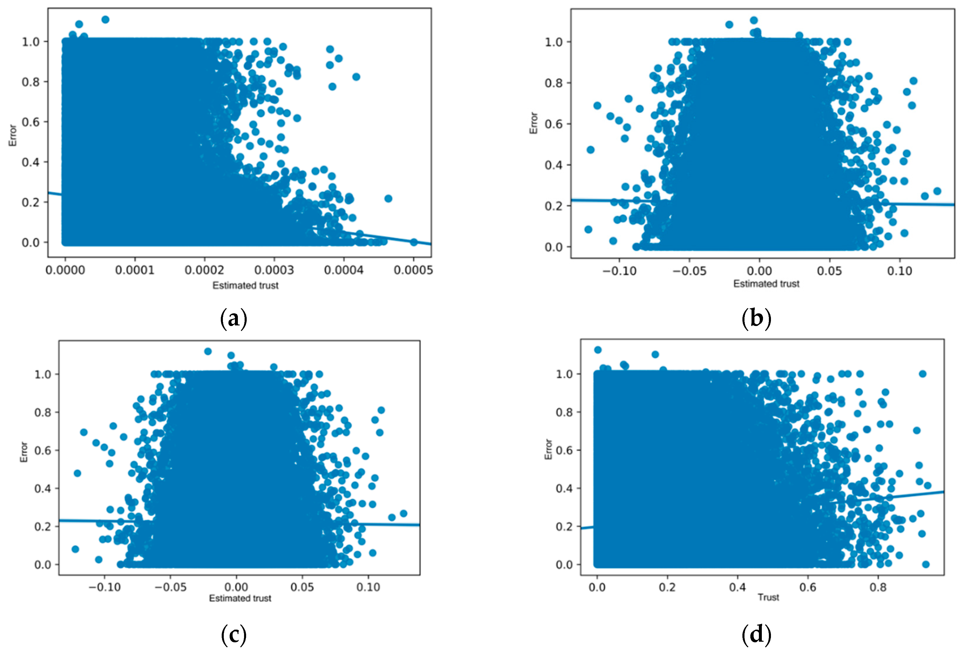
To determine the effect of trust on the accuracy of the test methods, we plotted the prediction error against the approximated or initial trust, as shown in Figure 3.

From all the trend lines of the graph in Figure 3a, it is clear that an increase in the estimated trust is associated with a low prediction error. However, in Figure 3b,c, the estimated trust, which is the same for S-Trust and W-Trust, consists of both positive and negative values. Since both the methods use the same trust, the two graphs seem almost identical. For these two methods, most of the data points are clustered around the center (the estimated trust value of zero). The trend line indicates that a slight increase in error is associated with increasing trust values. The I-Trust method also demonstrates the trend of increasing prediction error with increasing trust, as seen in Figure 3d. The slope of the trendlines indicates the strength of the association between trust values and errors. The M-Trust and I-Trust methods have a higher correlation than the S-Trust and W-Trust methods.

5.2. ML-1m

The results of the prediction accuracy as obtained by different methods are shown in Figure 4.

As for the previous data sets, the M-Trust demonstrates the best performance, with significant performance improvements compared to the baseline methods: 5.47% compared to SVD, 4.7% compared to SVD++, 48.09% compared to SocialMF, and 480.78% compared to NGCF. In contrast to the results of the previous data set, S-Trust has a considerably better improvement than that of W-Trust. Its improvements against the SVD, SVD++, SocialMF, and NGCF methods are 0.78%, 0.05%, 41.50%, and 458.45%, respectively. W-Trust does not exhibit any improvement against SVD and SVD++; however, its improvement against the SocialMF and NGCF methods are 39.9% and 451.57%, respectively. I-Trust maintains its status as in the previous data sets, and has performance improvements of 2.64%, 1.88%, 44.11%, and 468.74% compared to SVD, SVD++, SocialMF, and NGCF, respectively.

The results for the error–trust relationships, as shown in Figure 5, follow the same trends as those for other data sets.

5.3. ML-20m

The results of the experiments performed on the ML-20m data set are shown in Figure 6.

For this data set as well, M-Trust demonstrates the best performance with improvements compared to the baselines of 1.51% (SVD), 0.89% (SVD++), 24.04% (SocialMF), and 398.29% (NCGF). S-Trust and W-Trust demonstrate the same improvements. Both methods have improvements of 0.80%, 0.20%, 23.19%, and 394.87% compared to SVD, SVD++, SocialMF, and NGCF, respectively. Similar to the ML-100k data set, I-Trust demonstrates the second-best performance with an accuracy improvement of 1.09% compared to VD, 0.49% compared to SVD++, 23.54% compared to SocialMF, and 396.27% compared to NGCF.

Figure 7 shows the association between the error and trust in all the predicted ratings for the ML-20m data set.

As can be seen in Figure 7, the trust and error association is similar to that of the other data sets. In the next section, we further analyze how trust affects the final latent features.

5.4. Final Latent Features

The accuracy of predictions depends on how accurately we calculate the final latent features. These final features are derived from Equations (12)–(17). The mean values are calculated using both item and user features. For the three data sets, we have graphed the mean values of the final latent matrices, after combining them with estimated trusts, for M-Trust, S-Trust, and W-Trust. For I-Trust, we only use the initial trust.

In Figure 8, the mean values of the latent features in M-Trust are significantly greater than those of other methods; for all data sets, the values are around 0.045. This is due to the stacking of the mean trust value to the initial latent features. For the three data sets, M-Trust produces better accuracy than all the other methods. Consequently, stacking the mean trust values acts as adding preference biases to SVD or SVD++, resulting in better accuracy. Similarly, for I-Trust, when trust is combined with latent matrices, the mean values are increased. The I-Trust method has much higher values than that of the S-Trust and W-Trust methods, for all the data sets. This explains why the prediction accuracy of the I-Trust method is higher than that of both the S-Trust and W-Trust methods. The values in the latent matrices of both S-Trust and M-Trust are very small after combining trust. This is reflected in the results in all the prediction accuracy graphs (Figure 2, Figure 4 and Figure 6). These two methods’ prediction accuracies do not demonstrate significant improvements compared to those of SVD and SVD++. However, they are still better than those of SocialMF and NGCF.

6. Discussion

Please note that when reporting the effect of the trust or estimated trust on the predicted rating, we used the signed error instead of absolute error. This is because the association between the (estimated or initial) trust and error is considerably more visible when non-absolute error is used. Another critical point to note is that the proposed trust measure is heavily dependent on the number of users and items in the data set. Therefore, if the data set contains an extremely large number of items and users, and a user and item have very few ratings, none of the trust combination methods would have a significant influence on the predicted rating. A straightforward approach to address this problem is to use a subset of the full data sets to make the prediction. This approach is very common in real-world recommender systems, as the use of a full data set is not practical for some recommendation techniques [28]. Since the implicit trust calculations in our model are purely based on users’ preference, we expect the model to perform similarly on other domains such as music or product recommendations, as long as preference data is available. However, if the data sets have an extremely large number of items or users, the trust values may not have a significant effect on prediction values.

Here, we focused on the prediction accuracy of recommendation systems using implicit trust. We found that in terms of the prediction accuracy, the deep learning-based baseline method exhibits a considerably worse performance than the other three baselines. Similar to most modern recommendation techniques, NCGF is not designed to perform optimization for prediction accuracy, but instead for better prediction ranking. Therefore, as a future work, we plan to modify the proposed method to accommodate prediction ranking.

7. Conclusions

The use of side information such as trust in CF is a widely researched domain. However, the difficulty in determining explicit trust links means that researchers must infer trust links from the available preference data. A common approach is to use the PCC of the co-rated items as trust. However, this metric fails on binary data. Here, we inferred the trust from implicit rating data. Specifically, we proposed four trust-infused model-based CF techniques. Three of the four proposed methods determine the latent trust features, and then these latent features are combined with the latent features of the items and users. In the fourth method, the initially calculated trust values are used directly in the prediction stage to make recommendations. The proposed methods were tested against four baseline methods: SVD, SVD++, SocialMF, and NGCF. The experimental results demonstrate that the proposed methods significantly improve the prediction accuracy compared to that of the baseline methods. Among the proposed test methods, M-Trust performed the best. It achieved the best prediction accuracies for all data sets. I-Trust, which uses the initial trust at the prediction phase, achieves the second-best results. S-Trust and W-Trust performances are not as significant as those of M-Trust and I-Trust. However, they are still better than all the baseline methods.

References

- Resnick, P.; Iacovou, N.; Suchak, M.; Bergstrom, P.; Riedl, J. GroupLens: An open architecture for collaborative filtering of netnews. In Proceedings of the 1994 ACM Conference on Computer Supported Cooperative Work, Chapel Hill, NC, USA, 22–26 October 1994; pp. 175–186. [Google Scholar]
- Lathia, N.; Hailes, S.; Capra, L. Trust-based collaborative filtering. In Proceedings of the IFIP International Conference on Trust Management, Trondheim, Norway, 18–20 June 2008; pp. 119–134. [Google Scholar]
- Guha, R.; Kumar, R.; Raghavan, P.; Tomkins, A. Propagation of trust and distrust. In Proceedings of the 13th International Conference on World Wide Web, New York, NY, USA, 17–22 May 2004; pp. 403–412. [Google Scholar]
- O’Donovan, J.; Smyth, B. Trust in Recommender Systems. In Proceedings of the 10th International Conference on Intelligent User Interfaces, San Diego, CA, USA, 10–13 January 2005. [Google Scholar]
- Meyer, F. Recommender Systems in Industrial Contexts. Ph.D. Thesis, Grenoble Alpes University, Grenoble, France, 2012. [Google Scholar]
- Koren, Y.; Bell, R.; Volinsky, C. Matrix Factorization Techniques for Recommender Systems. Computer 2009, 8, 30–37. [Google Scholar] [CrossRef]
- Srebro, N.; Jaakkola, T. Weighted low-rank approximations. In Proceedings of the 20th International Conference on Machine Learning (ICML-03), Washington, DC, USA, 21–24 August 2003; pp. 720–727. [Google Scholar]
- Lee, J.; Kim, S.; Lebanon, G.; Singer, Y. Local low-rank matrix approximation. In Proceedings of the International Conference on Machine Learning, Atlanta, GA, USA, 16–21 June 2013; pp. 82–90. [Google Scholar]
- Mackey, L.W.; Jordan, M.I.; Talwalkar, A. Divide-and-conquer matrix factorization. In Proceedings of the Advances in Neural Information Processing Systems, Granada, Spain, 12–17 December 2011; pp. 1134–1142. [Google Scholar]
- Massa, P.; Avesani, P. Trust-aware recommender systems. In Proceedings of the 2007 ACM Conference on Recommender Systems, Minneapolis, MN, USA, 19–20 October 2007; pp. 17–24. [Google Scholar]
- Page, L.; Brin, S.; Motwani, R.; Winograd, T. The PageRank Citation Ranking: Bringing Order to the Web; Technical Report; Stanford InfoLab: Santa Clara, CA, USA, 1999. [Google Scholar]
- Golbeck, J.; Hendler, J. Filmtrust: Movie recommendations using trust in web-based social networks. In Proceedings of the IEEE Consumer Communications and Networking Conference, Las Vegas, NV, USA, 8–10 January 2006; Volume 96, No. 1. pp. 282–286. [Google Scholar]
- Zahir, A.; Yuan, Y.; Moniz, K. AgreeRelTrust—A Simple Implicit Trust Inference Model for Memory-Based Collaborative Filtering Recommendation Systems. Electronics 2019, 8, 427. [Google Scholar] [CrossRef]
- Ma, X.; Lu, H.; Gan, Z. Improving recommendation accuracy by combining trust communities and collaborative filtering. In Proceedings of the 23rd ACM International Conference on Conference on Information and Knowledge Management, Shanghai, China, 3–7 November 2014; pp. 1951–1954. [Google Scholar]
- Bell, R.M.; Koren, Y. Improved neighborhood-based collaborative filtering. In Proceedings of the KDD-Cup and Workshop 2007, San Jose, CA, USA, 12 August 2007; pp. 7–14. [Google Scholar]
- Niu, M.; Qu, Y.; Cao, X.; Tang, R.; He, X.; Yu, Y. Collaborative Filtering with Graph-based Implicit Feedback. In Proceedings of the 2017 International Conference on Computer Technology, Electronics and Communication (ICCTEC), Dalian, China, 19–21 December 2017; pp. 328–335. [Google Scholar]
- Latapy, M.; Tchuenté, M.; Nzekon, N.; Jacques, A. A general graph-based framework for top-N recommendation using content, temporal and trust information. J. Interdiscip. Methodol. Issues Sci. 2019, 5. [Google Scholar] [CrossRef]
- Papagelis, M.; Plexousakis, D.; Kutsuras, T. Alleviating the sparsity problem of collaborative filtering using trust inferences. In Proceedings of the International Conference on Trust Management, Paris, France, 23–26 May 2005; pp. 224–239. [Google Scholar]
- Salakhutdinov, R.; Mnih, A.; Hinton, G. Restricted Boltzmann machines for collaborative filtering. In Proceedings of the 24th International Conference on Machine learning, Corvalis, OR, USA, 20–24 June 2007; pp. 791–798. [Google Scholar]
- Betru, B.T.; Onana, C.A.; Batchakui, B. Deep learning methods on recommender system: A survey of state-of-the-art. Int. J. Comput. Appl. 2017, 162, 17–22. [Google Scholar]
- Wang, X.; He, X.; Wang, M.; Feng, F.; Chua, T.-S. Neural Graph Collaborative Filtering. In Proceedings of the 42nd International ACM SIGIR Conference on Research and Development in Information Retrieval, Paris, France, 21–25 July 2019; pp. 165–174. [Google Scholar]
- Ma, H.; King, I.; Lyu, M.R. Learning to recommend with social trust ensemble. In Proceedings of the 32nd International ACM SIGIR Conference on Research and development in Information Retrieval, Boston, MA, USA, 19–23 July 2009; pp. 203–210. [Google Scholar]
- Jamali, M.; Ester, M. A matrix factorization technique with trust propagation for recommendation in social networks. In Proceedings of the 4th ACM Conference on Recommender Systems, Barcelona, Spain, 26–30 September 2010; pp. 135–142. [Google Scholar]
- Forsati, R.; Mahdavi, M.; Shamsfard, M.; Sarwat, M. Matrix factorization with explicit trust and distrust side information for improved social recommendation. ACM Trans. Inf. Syst. 2014, 32, 17. [Google Scholar]
- Harper, F.M.; Konstan, J.A. The movielens datasets: History and context. Acm Trans. Interact. Intell. Syst. 2016, 5, 19. [Google Scholar] [CrossRef]
- Pitsilis, G.; Marshall, L.F. A Model of Trust Derivation from Evidence for Use in Recommendation Systems; University of Newcastle upon Tyne, Computing Science: Newcastle upon Tyne, UK, 2004; pp. 1–10. [Google Scholar]
- Hug, N. Surprise, a Python library for recommender systems. 2017. Available online: www.surpriselib.com (accessed on 12 July 2019).
- He, X.; Liao, L.; Zhang, H.; Nie, L.; Hu, X.; Chua, T.-S. Neural collaborative filtering. In Proceedings of the 26th International Conference on World Wide Web, Perth, Australia, 3–7 April 2017; pp. 173–182. [Google Scholar]
Figure 1.
Rating matrix approximation with latent features.
Figure 2.
Prediction accuracy obtained using different methods for the ML-100k data set. MAE: Mean absolute error; SVD: Singular value decomposition; NGCF: Neural graph collaborative filtering.
Figure 3.
Errors in predictions versus trust (or estimated trust) for the ML-100k data set, corresponding to different methods. (a) Mean estimated trust against signed error in rating prediction using M-Trust. (b) Estimated trust against signed error in rating prediction using S-Trust. (c) Estimated trust against signed error in rating prediction using W-Trust. (d) Initial trust against signed prediction error for I-Trust.
Figure 4.
Prediction accuracy for the ML-1m data set, obtained using different comparison methods.
Figure 5.
Errors in predictions versus trust (or estimated trust) for the ML-1m data set, as obtained by different methods: (a) Estimated trust against signed error in rating prediction using M-Trust; (b) Estimated trust against signed error in rating prediction using S-Trust; (c) Estimated trust against signed error in rating prediction using W-Trust; (d) Initial trust against signed prediction error for I-Trust.
Figure 6.
Prediction accuracy for ML-20m data set, as obtained using different methods.
Figure 7.
Errors in predictions versus trust (or estimated trust) for the ML-20m data set, as obtained by different methods: (a) Estimated trust against signed error in rating prediction using M-Trust; (b) Estimated trust against signed error in rating prediction using S-Trust; (c) Estimated trust against signed error in rating prediction using W-Trust; (d) Initial trust against signed prediction error for I-Trust.
Figure 8.
Mean values of latent matrices in proposed methods.