Analysis of a Collision-Energy-Based Method for the Prediction of Ice Loading on Ships

Abstract

Ships designed for operation in Polar waters must be approved in accordance with the International Code for Ships Operating in Polar Waters (Polar Code), adopted by the International Maritime Organization (IMO). To account for ice loading on ships, the Polar Code includes references to the International Association of Classification Societies’ (IACS) Polar Class (PC) standards. For the determination of design ice loads, the PC standards rely upon a method applying the principle of the conservation of momentum and energy in collisions. The method, which is known as the Popov Method, is fundamentally analytical, but because the ship–ice interaction process is complex and not fully understood, its practical applications, including the PC standards, rely upon multiple assumptions. In this study, to help naval architects make better-informed decisions in the design of Arctic ships, and to support progress towards goal-based design, we analyse the effect of the assumptions behind the Popov Method by comparing ice load predictions, calculated by the Method with corresponding full-scale ice load measurements. Our findings indicate that assumptions concerning the modelling of the ship–ice collision scenario, the ship–ice contact geometry and the ice conditions, among others, significantly affect how well the ice load prediction agrees with the measurements.

1. Introduction

Maritime activity in the Arctic is on the increase, driven by the extraction of Arctic natural resources, trans-Arctic shipping and Arctic tourism. To manage related risks, the maritime industry must ensure that Arctic ships are safe and sustainable. To this end, ships operating in Polar water must be approved under the International Code for Ships Operating in Polar Waters, or the Polar Code [1], enforced by the International Maritime Organization (IMO). The specific objective of the Polar Code is to ensure the same level of safety for ships, persons and the environment in Polar waters, as in other waters [2]. Towards this end, it supplements the International Convention for the Safety of Life at Sea (SOLAS) and the International Convention for the Prevention of Pollution from Ships (MARPOL) to account for Arctic-specific safety hazards, such as sea ice, icing, low temperatures, darkness, high latitude, remoteness, the lack of relevant crew experience and difficult weather conditions.

A ship approved in accordance with the Polar Code is issued a Polar Ship Certificate that classifies the ship as one of the following:

• Category A, for ships allowed to operate in at least medium-thick first-year ice.
• Category B, for ships allowed to operate in at least thin first-year ice.
• Category C, for ships allowed to operate in ice conditions less severe than those included in Categories A or B.

In addition to the ship’s category, the ice certificate determines detailed operational limits concerning, for instance, the minimum temperature and the worst ice conditions in which a ship can operate.

The Polar Code is fundamentally goal-based, determining mandatory provisions in terms of goals, functional requirements FR(s), and regulations to meet those goals. As a result, a ship can be approved either as a prescriptive design or as an equivalent design. A prescriptive design is a design that meets all of the prescriptive regulations associated with the FR(s), whereas an equivalent design is a design that is approved in accordance with Regulation 4 of SOLAS Chapter XIV. The latter case results in a so-called alternative or equivalent design. Per regulation 4—“Alternative design and arrangement” of SOLAS Chapter XIV [3], where alternative or equivalent designs or arrangements are proposed, they are to be justified by the following IMO Guidelines:

• “Guidelines for the approval of alternatives and equivalents as provided for in various IMO instruments”, MSC.1/Circ.1455 [4].
• “Guidelines on alternative design and arrangements for SOLAS chapters II-1 and III, MSC.1/Circ.1212 [5].
• “Guidelines on alternative design and arrangements for fire safety”, MSC/Circ.1002 [6].

A general principle is that any alternative design should be at least as safe as a design determined by prescriptive rules. Many of the prescriptive regulations of the Polar Code, in particular, those related to a vessel’s structural strength, include references to the International Association of Classification Societies’ (IACS) Polar Class (PC) ice class standards [7]. These consist of in total seven PC notations, ranging from PC 1 (highest) to PC 7 (lowest), corresponding to various levels of operational capability in ice and hull strength. For instance, as per the Polar Code, for a Category A ship to meet FR(s) regarding structural strength, the ship must be constructed in accordance with PC 1–5, whereas a Category B ship must be constructed in accordance with PC 6–7. Alternatively, the scantlings must be determined in accordance with a standard which offers an equivalent level of safety following the above-described principle of design equivalency.

Because the ship–ice interaction process is complex, stochastic and not fully understood, predicting the level of ice loading that a ship will be exposed to is challenging. Multiple different methods to predict ice loading have been proposed, including analytical, numerical and empirical methods [8]. However, to date, none of the existing methods can be considered complete and sufficiently validated to enable them to support direct goal-based structural design following the Polar Code. Thus, in practice, designers are dependent upon the application of the PC standards to obtain regulatory approval for ships designed for operation in ice-infested waters.

For the assessment of design ice loading, the PC standards apply a method based on the principle of the conservation of momentum and energy in collisions, presented by Popov, et al. [9]. The method, in the following referred to as the Popov Method, is relevant for the assessment of ice loading on ships interacting with all types of sea ice. Despite the method being fundamentally analytical, its practical applications, including its application in the PC standards, rely on several assumptions. These concern the modelling of the collision scenario (e.g., type of collision, ship–ice contact geometry), as well as the material properties of ice [10,11]. Because many of the assumptions are empirically determined, the PC standards can be considered semi-empirical, meaning that they might not be efficient when applied on design and operating conditions different from those for which the assumptions were determined [12].

Against this background, this study aims to help designers to make better-informed decisions in the design of Arctic ships by analysing the role and effects of the collision scenario assumptions behind the application of the Popov Method [9]. Specifically, the study addresses the following research questions:

• How do assumptions behind the modelling of the collision scenario and the description of the operating conditions affect the ice load estimate?
• What collision scenario assumptions should be applied to obtain reliable ice load estimates for typical operation in level and broken ice?

Because the Popov Method in principle makes it possible to assess ice loading for a wide range of ship designs and operating scenarios, the method is highly relevant in the context of goal-based design. Thus, by addressing the above research questions, we also aim to support progress towards the goal-based design of Arctic ships, as per the above-described principle of equivalent design.

The study is limited to issues concerning ice material properties and non-accidental ship–ice interactions resulting in no or minor structural deformation with relatively thick ice, where the dominant failure mode is crushing. We do not consider the following:

• Issues concerning hydrodynamic effects. These are assumed to have a limited effect on the types of collision scenarios considered [13].
• Issues concerning structural resistance.
• Local plastic deformations. Thus, although the method can do so, we do not consider local plastic deformations, which could affect the obtained load estimate [14,15]. It can be mentioned that allowable plastic deformations are not clearly defined in the PC rules [16].
• Interactions with thin ice, which in addition to crushing would require the consideration of flexural failure and dynamic effects [17]. Daley & Kendrick [18] indicate that when dynamic effects are considered, the design normal force is increasing with increasing impact velocity [6].
• Secondary impacts (i.e., reflected collisions). Daley & Liu [19], among others, demonstrate that when operating in thick ice, reflected collisions may result in critical loads, in particular on the mid-ship area.
• Moving loads along the hull that may result from a collision with pack ice, glacial ice, or ice channel edges are not considered. Kendrick et al. [20] and Quinton & Daley [21] indicate that moving ice loads may cause more damage than stationary loads of similar magnitude. Consideration of moving loads would require the consideration of additional factors such as sliding contact, nonlinear geometric and material behaviours in structural components, requiring the application of the finite element analysis [22].

2. Background

2.1. The Popov Method

The Popov Method models the ship–ice interaction process as an equivalent one-dimensional collision with all motions taking place along the normal to the shell at the point of impact [23]. The model does not consider sliding friction and buoyancy forces. A single hydrodynamic effect, namely the added mass of the surrounding water, is considered.

To simplify the ship–ice interaction process to an equivalent one-dimensional collision, Popov et al. [9] introduce the so-called “reduced mass” concept [23]. Accordingly, the total reduced mass $M_{red},\left[t\right]$ of the ship–ice system is derived by coupling 6-degree of freedom (DOF) equations describing the motions of a ship with 3-DOF equations describing the motions of an ice floe [9]. By assuming that ice floes are of an ellipsoid shape, the 6-DOF and 3-DOF models are converted into a model with a single DOF. As a result, the contact force $F,\left[MN\right]$ can be determined as an integral of contact pressure over the nominal contact area $A,\left[m^2\right]$ per

$$M_{red}\frac{{\mathrm{d}}^2}{\mathrm{d}{t}^2}{\mathsf{\zeta }}_n\left(t\right)·{10}^{-3}=F={\displaystyle \int }p\left({\mathsf{\zeta }}_n,\frac{\mathrm{d}}{\mathrm{d}t}{\mathsf{\zeta }}_n\left(t\right)\right)dA,\left[MN\right]$$

(1)

where ${\mathsf{\zeta }}_n,\left[m\right]$ is indentation depth, $t,\left[sec\right]$ is time, and $p\left({\mathsf{\zeta }}_n,\dot{{\mathsf{\zeta }}_n}\right),\left[MPa\right]$ is “contact pressure” [9]. The initial impact conditions at $t=0$ are as follows: ${\zeta }_n\left(0\right)=0$ and $\dot{{\zeta }_n}\left(0\right)=v_1$, where $v_1$ is the reduced speed for the ship $\left[m/sec\right]$. At the end of the interaction at $t=t_{max}$ the following conditions apply: ${\zeta }_n\left(t_{max}\right)={\zeta }_{max}$ and $\dot{{\zeta }_n}\left(0\right)=0$.

The ship–ice contact area depends on the hull form, assumed shape of the ice edge and the assumed indentation of the ship into the ice.

$$A=G{\mathsf{\zeta }}_n{}^a,\left[m^2\right]$$

(2)

where $G$ is a coefficient depending on the geometric parameters of the ship and the ice, and $a$ is an exponent depending on the assumed shape of the ice edge at the point of impact [9]. This means that the relationship between the normal indentation and the nominal contact area can be determined for any contact geometry.

2.2. Collision Scenario

In an ice floe-structure interaction, there are three limit mechanisms for ice loads: Limit ice strength, limit driving force and limit momentum [24]. The Popov Method is based on the mechanisms of limit momentum, also referred to limit energy mechanism, and it considers impacts between two bodies where one body is initially moving and the other is at rest. The ice load is calculated by equating the available kinetic energy with the energy expended in crushing and the potential energy in collisions.

Due to the non-homogeneous nature of sea ice and the complexity of the ship–ice interaction process, the number of possible ship–ice collision scenarios is large. Thus, when predicting ice loading, assumptions must be made regarding the location of the ship–ice impact (e.g., bow, side, stern), the type of ice involved (e.g., ice floe, ice field), and the resulting contact geometries [11]. Popov et al. [9] consider the following ship–ice collision scenarios:

• An impact between a ship and an ice floe. According to Enkvist, et al. [25] this is the most common collision scenario for merchant ships. As per

  Table 1. Energy components of the Popov Method as determined based on Popov et al. [9]).

  Case 1: Ship–Ice Floe Collision	Case 2: Ship–Ice Field Collision
  $T_1+T_2=U$	$T_1=U+V$
  $T_1=1/2·M_{red}{}^{ship}·v_1{}^2$	$T_1=1/2·M_{red}{}^{ship}·v_1{}^2$
  $T_2=1/2·M_{red}{}^{ice}·v_2{}^2$	$V=1/2·f·P_v$
  $U={{\displaystyle \int }}_0^{{\mathsf{\zeta }}_n}Fd{\mathsf{\zeta }}_n$	$U={{\displaystyle \int }}_0^{{\mathsf{\zeta }}_n}Fd{\mathsf{\zeta }}_n$

  , in this scenario, the kinetic energy of the ship $T_1,\left[J\right]$ is partially converted into the kinetic energy of the ice floe $T_2,\left[J\right]$ and partially consumed in crushing the ice edge $U,\left[J\right]$. $T_1$, $T_2$, and $U$ are calculated in accordance with the formulas presented in Table 1 (Case 1), where $M_{red}{}^{ship},\left[t\right]$ and $M_{red}{}^{ice},\left[t\right]$ are the reduced masses of the ship and the ice floe, and the parameters $v_1,\left[m/sec\right]$ and $v_2,\left[m/sec\right]$ correspond to the reduced speeds of the ship and the ice floe.
• An impact between a ship and the edge of an ice field. In this scenario, defined as case two in Table 1, the edge of the ice field is crushed, and the ice field bends due to the vertical component of the contact force $P_v,\left[N\right]$. In this scenario, the ship’s kinetic energy $T_1,\left[J\right]$ is consumed by the crushing $U,\left[J\right]$ and by the bending of the ice field $V,\left[J\right]$. $T_1$, $V$, and $U$ are calculated in accordance with the formulas presented in Table 1 (Case 2), where $f=\frac{P_v}{2·\sqrt{{\gamma }_i·D}}\left[m\right]$, ${\gamma }_i,\left[N/m^3\right]$ is the specific weight of ice, $D=\frac{E·h_i^3}{12·\left(1-\mu \right)},\left[Pa·m^3\right]$ is flexural stiffness of an ice plate, $E,\left[Pa\right]$ is the elastic modulus of ice, $h_i,\left[m\right]$ is the ice thickness, $\mu$ is Poisson ratio for ice.

2.3. Ship–Ice Contact and Ice Crushing Pressure

To manage the complexity of the ship–ice interaction process, ship–ice contact forces can be estimated based on the average pressure and contact area in terms of so-called pressure-area models [26]. These are typically presented in the form of pressure-area relationships $P\left(A\right)$ describing the development of the average pressure throughout the ice indentation process [27,28]. Because the ship–ice interaction process is complex and not fully known, $P\left(A\right)$ relationships can only be reliably determined based on full-scale measurements.

The maximum force generated by ice acting upon a structure depends on the strength of the ice in the relevant mode of failure [29]. Because in ship–ice interactions, the ice often fails by crushing, ice crushing strength is an important factor for estimating ice loading on ships [30]. As pointed out by Kujala [8], the crushing strength of ice depends on multiple parameters, including ice salinity, ice temperature and loading rate, but all of this is not fully understood. However, as demonstrated empirically by Michel and Blanchet [31], ice crushing strength is proportional to ice compressive strength ${\sigma }_{co},\left[MPa\right]$ as per

$${\sigma }_{cr}=C·{\sigma }_{co},\left[MN\right]$$

(3)

where $C$ is an indentation coefficient which for the brittle range for sea ice has an empirically determined value of 1.57 [32,33].

2.4. Contact Geometry

To calculate ice loads using the Popov Method, the ship’s indentation into the ice must be defined. Following Tunik [11], the indentation can be assessed based on the assumed form of the contact area between the ship and the ice, which depends both on the form of the ship’s hull, and on the form of the ice at the point of impact. Per the Popov Method, this form is modelled in terms of an ice–hull overlap geometry, in the following referred to as contact geometry [34].

In real-life ship–ice interactions, many different types of contact geometries occur. Thus, to enable the assessment of ice loading from different types of ship–ice interactions, Popov et al. [9], Daley [34] and Daley & Kim [35] present contact geometry models corresponding to different ship–ice interactions. A selection of these contact geometries are presented in Figure 1, and explained in the following:

• Round contact geometry. This model, which is behind the design scenario of the ice class standards of the Russian Maritime Register of Shipping (RMRS), corresponds to an oblique collision with a rounded ice edge [12]. Related geometrical parameters are the radius of ice floe $\mathrm{R},[m$], the waterline angle $\alpha ,\left[deg\right]$ and normal frame angle ${\beta }^{\prime },\left[deg\right]$. Parameters $\alpha$ and ${\beta }^{\prime }$ are dependent on the hull form, whereas R is dependent on the ice conditions. In the RMRS ice class rules, R is assumed at $25m$.
• Angular (wedge) contact geometry. This model is applied in the design scenario of the PC rules [14]. Related geometrical parameters are the ice edge opening angle $\mathsf{\varphi },\left[deg\right]$, waterline angle $\alpha ,\left[deg\right]$ and normal frame angle ${\beta }^{\prime },\left[deg\right]$. According to Popov, et al. [9], $\mathsf{\varphi }$ can be determined by observation of ice segments broken by a ship. Alternatively, $\mathsf{\varphi }$ can be determined by numerical simulations [36].
• Symmetric v wedge contact geometry. This model can be applied to assess ice loads from beaching impacts, i.e., when a ship is ramming an ice sheet so that the bow of the ship rises upwards onto the ice sheet [34]. Related geometrical parameters are waterline angle $\alpha ,\left[deg\right]$, frame angle $\beta ,\left[deg\right]$ and stem angle $\mathsf{\gamma },\left[deg\right]$, all of which depend on the hull form at the point of impact.
• Right-apex oblique contact geometry. This model, defined by Daley [34], corresponds to continuous operation in ice without ramming. Related geometrical parameters are waterline angle $\alpha ,\left[deg\right]$, normal frame angle ${\beta }^{\prime },\left[deg\right]$, stem angle $\mathsf{\gamma },\left[deg\right]$ and frame angle $\beta ,\left[deg\right]$, all of which depend on the hull form at the point of impact.
• Spherical contact geometry. This model can be applied for the assessment of ice loads on a bulbous bow [20]. Related geometrical parameters are the contact radius $\mathrm{r},\left[m\right]$, waterline angle $\alpha ,\left[deg\right]$ and the normal frame angle ${\beta }^{\prime },\left[deg\right]$, all of which depend on the hull form at the point of impact.
• Pyramid contact geometry. This model can be applied to assess ice loads from ship–iceberg interactions resulting in structural deformations [35]. Related geometrical parameters are the ice edge opening angle $\mathsf{\varphi },\left[deg\right]$, waterline angle $\alpha ,\left[deg\right]$ and normal frame angle ${\beta }^{\prime },\left[deg\right]$.

As per the contact geometries presented above, the level of ice loading might depend on the hull form in terms of the frame angle $\beta$, waterline angle $\alpha$ and stem angle $\mathsf{\gamma }$, as shown in Figure 1. Generally, a reduced frame angle, an increased waterline angle, or an increased stem angle result in higher ice loads, and vice versa. However, as discussed by Popov, et al. [9] the influence of the different angles depends upon the point of impact.

2.5. Identification of Assumptions Behind the Popov Method and the PC Rules

Based on Popov et al. [9], Dolny [14], Daley [10], Daley et al. [37] and IACS [38] we identify the following assumptions behind the Popov Method and the related PC rules:

• Assumptions related to the definition of the ship–ice collision scenario. The Popov Method assumes two types of ship–ice collision scenarios defined in Table 1: (a) Ship–ice floe collision, and (b) ship–ice field collision. The PC rules, on the other hand, assume a single type of ship–ice collision scenario, namely a glancing impact with thick level ice.
• Assumptions related to the definition of contact pressure. For typical speeds of ships operating in ice, Popov et al. [9] suggested that the contact pressure $p\left({\mathsf{\zeta }}_n,\dot{{\mathsf{\zeta }}_n}\right)$ can be assumed equal to the ice crushing strength ${\sigma }_{cr},\left[MPa\right]$ over the whole contact area. Accordingly, the maximum ice load corresponding to the maximum indentation depth ${\mathsf{\zeta }}_{max},\left[m\right]$ can be defined as per

  $$F={\sigma }_{cr}{{\displaystyle \int }}_0^{{\mathsf{\zeta }}_{max}}dA,\left[MN\right]$$

  (4)

  However, this is a simplification, as the crushing strength of ice depends on multiple factors and varies between $1.25-10MPa$ [9]. In the PC rules, on the other hand, the contact pressure is assumed to correspond to the pressure-area relationship following:

  $$P=P_0{A}^{ex},\left[MPa\right],$$

  (5)

  where $P_0,\left[MPa\right]$ is average pressure acting on 1 $m^2$ (class dependent), $A,\left[m^2\right]$ is the contact area, and $ex$ is a coefficient empirically determined as −0.1.
• Assumptions related to the definition of the contact geometry case. The application of specific contact geometries requires making assumptions regarding individual contact geometry parameters. When applying the round contact geometry model, Popov et al. [9] recommend the use of R-values in the range of 10–40 m. For angular contact geometry, Popov et al. [9] recommend the use of ice opening angle values ($\mathsf{\varphi }$) in the range of 45°–145°. In the PC rules the assumed contact geometry case is always angular (also referred to as a wedge shape) with a constant $\mathsf{\varphi }$ value of 150° [37].
• Assumptions related to the definition of the size of the nominal ship–ice contact area. As per the Popov Method, the nominal ship–ice contact area is assumed to be dependent on the form of the hull and ice at the point of impact as per Equation (2). The PC rules, on the other hand, assuming a wedge-shaped contact geometry, assume a single nominal contact area defined per

  $$A=\frac{{\mathsf{\zeta }}_n{}^2·\tan \left(\frac{\mathsf{\varphi }}{2}\right)}{{(\cos {\beta }^{\prime })}^2·\sin {\beta }^{\prime }}\left[m^2\right]$$

  (6)

  Naturally, this is a simplification as the actual contact area depends strongly on the assumed contact geometry, and thus on the prevailing ice conditions and the hull form.
• Assumptions related to the definition of load length and load height. The load length and load height, both of which affect the structural requirements in accordance with the PC rules, are derived as a function of the indentation depth [34,39]. In the PC rules, the design load length $w$ is assumed to be defined per

  $$w=W_{nom}{}^{wex},\left[m\right]$$

  (7)

  where $W_{nom}$ is the nominal contact length of the assumed wedge-shaped contact geometry and $wex$ is an ice spalling parameter with an empirically determined value of 0.7. The ice spalling parameter accounts for ice edge spalling effects by reducing the size of the contact patch. Although this parameter has a significant effect on the determined scantling requirements, no justification for the assumed value of $wex$ is found in the literature [12]. The design load height $h_d$ is related to the design load length as per

  $$h_d=\frac{w}{AR},\left[m\right]$$

  (8)

  where $AR$ is a design patch aspect ratio used to simplify the nominal contact area to an equivalent area of a rectangular patch.

3. Research Method

3.1. Ship–ice Interaction and Material Parameters

We determine the actual ice conditions and loads based on full-scale ice measurements and visual observations of the prevailing ice conditions conducted on the Polar Class 5 classified polar research ship S.A. Agulhas II on a voyage in the Antarctic Ocean in the period November 2013–February 2014 [40]. For the purpose of ice load measurements, the ship’s hull was instrumented in accordance with Figure 2 with strain gauges at the bow (frames 134 and 134.5), bow shoulder (frames 112 and 113), and stern shoulder (frames 39.5, 40, 40.5, and 41) [40]. The prevailing ice conditions were measured using a stereo camera.

The full-scale data describes the ship–ice interaction process and the prevailing operating conditions in terms of [40]:

• Ship parameters including hull particulars: Length, beam, draft, displacement, hull angles.
• Impact parameters including impact location and speed.
• Environmental parameters including ice floe size, ice thickness and air temperature.

From the full-scale data, we extract two data series for two separate operating days representing different types of ice conditions and operating modes:

• Data set A. Measurements from 10.12.2013 representing continuous operation in ice as well as specific manoeuvres such as ramming and reversing in ice. An extract of data set A is presented in Figure 3.
• Data set B. Measurements from 20.12.2013 representing mainly continuous operation in ice. An extract of data set A is presented in Figure 4.

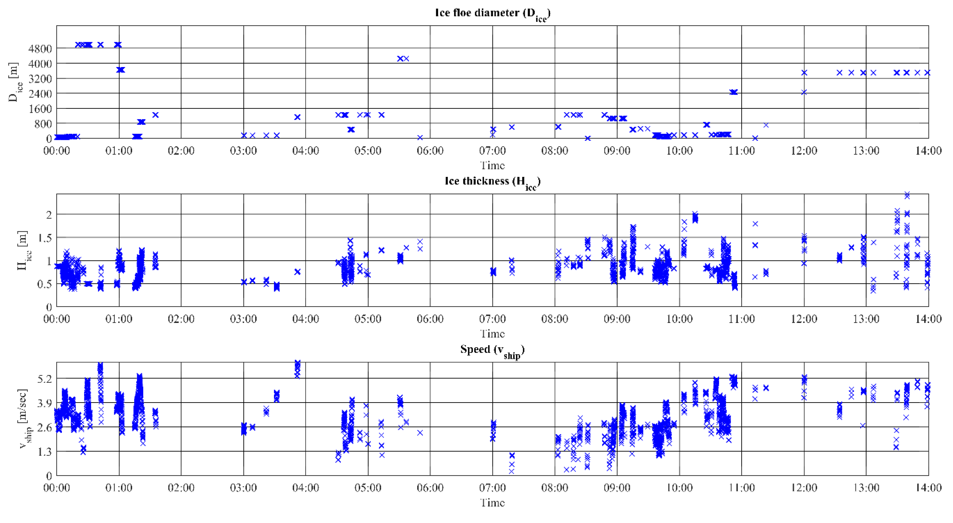
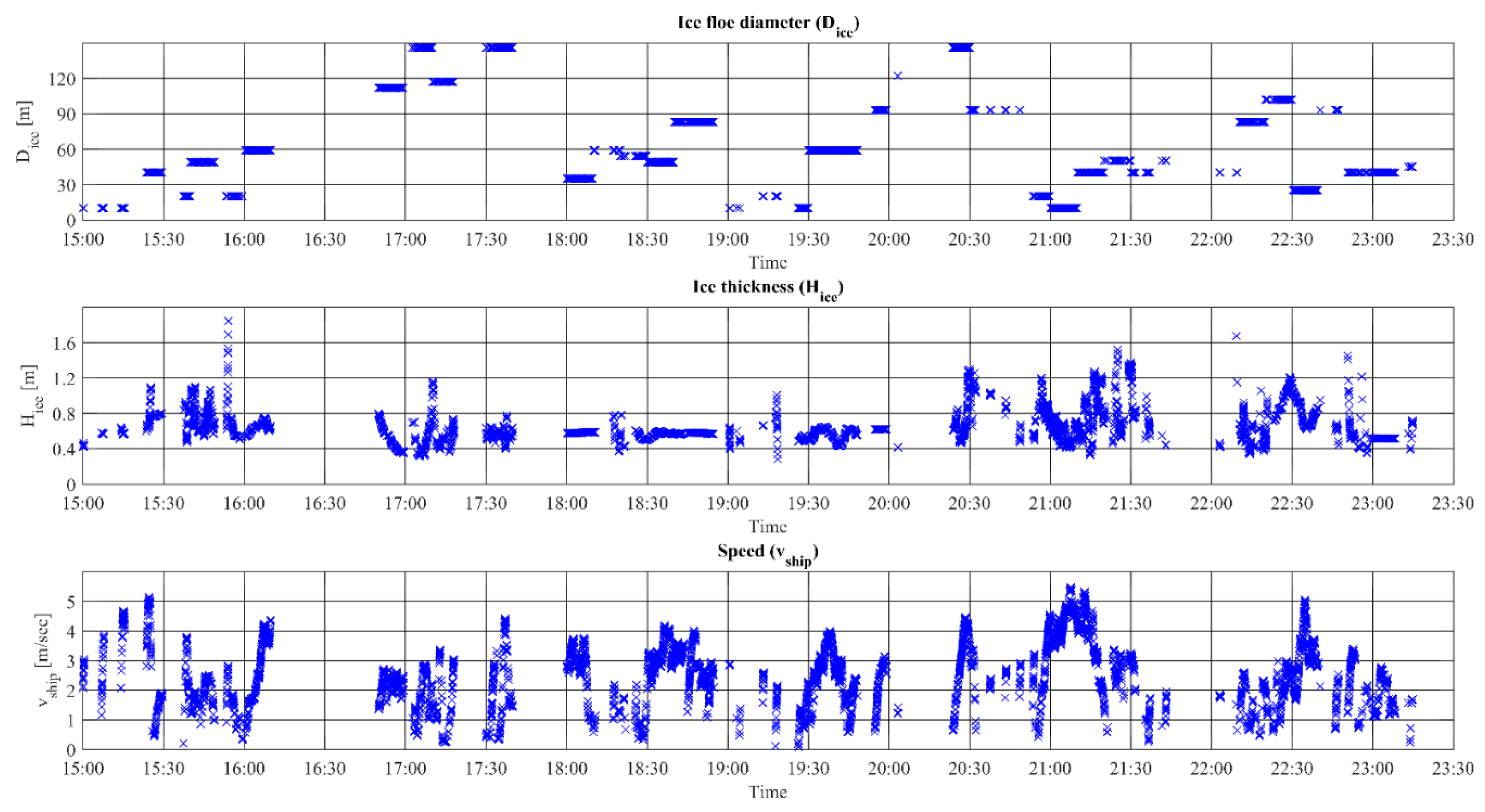
The specified ice floe diameters were determined by visual observations from the ship carried out every 10 or 15 min [41]. Because the measurements were carried out by visual observation, and because the size of individual ice floes were specified by categories of diameter range (e.g., 0–20 m, 20–100 m, 100–500 m), the diameter values specified in Figure 3 and Figure 4 are subject to significant uncertainty.

As mentioned in Sec. 2.5, ice crushing strength ${\sigma }_{cr}$ is an important factor for estimating ice loading on ships. In order to enable a direct comparison between the measured and calculated ice loads, accounting for the fact that ${\sigma }_{cr}$ depends on the prevailing environmental conditions, we calculate ${\sigma }_{cr}$ as function of ice salinity, brine volume, ice temperature, ice density and indentation rate in accordance with an approach proposed by Idrissova, et al. [42]. This approach assumes among others that ice crushing strength is proportional to the compressive strength of ice as suggested by Michel & Blanchet [31].

3.2. Collision Scenarios

Following Popov, et al. [9], collision scenarios are defined in terms of the impact location, type of collision (e.g., collision with an ice floe or an ice sheet) and contact geometry. Naturally, these are interlinked, because both the type of collision and the impact location affect the resulting contact geometry. Towards addressing our research questions, we analyse multiple collision scenarios defined by

Table 2. Collision scenarios proposed by Popov et al. [9] and Daley [34].

Impact Location	Bow Area, Where the Frame Angle is Larger than $10\left[\mathit{deg}\right]$
Types of collisions	(a) Glancing impact with an ice floe, (b) Glancing impact with an ice field
Contact geometries	Round, angular, symmetric v wedge, right-apex oblique

.

Per Table 2, we focus on the bow area because it is typically subjected to the largest ice loads. Specifically, based on the available full-scale data, we analyse ice loading on two specific impact locations in the bow area, namely frames 134 and 134.5. We focus on two of the most common types of collisions, namely glancing impact with an ice floe and glancing impact with an ice field. We consider four different types of contact geometry, namely round, angular (with ice edge opening angle of 145°), symmetric v wedge and right-apex oblique.

We do not consider pyramid and spherical contact geometries, because we assume that these are preliminary intended for the analysis of ship-iceberg and bulbous bow-ice impacts [20,35].

We confirmed this assumption by calculations indicating that the applications of the pyramid and spherical contact geometries result in ice load predictions that are multiple times higher than the corresponding measurements.

3.3. Ice Load Parameters

To calculate ice-crushing pressure $p,\left[MPA\right]$, we first need to calculate related ice load parameters including indentation depth, contact area, normal force and load length. We calculate indentation depth directly by the Popov Method for all considered collision scenarios. To this end, we apply the contact geometry specific values for $G$ and $a$ (see Equation (2)) determined by Popov, et al. [9], Daley [34] and Daley & Kim [35]. We then calculate the ship–ice contact area $A,\left[m^2\right]$, following Equation (2), then the related load length $l,\left[m\right]$ and the total ice load $F,\left[MN\right]$, following Equation (4). The load length is thereby specific for each contact geometry and can be derived as a function of the indentation depth. For example, for round contact geometry, load length $l_{round},\left[m\right]$ is calculated following Equation (9) [9].

$$l_{round}=\frac{5}{3}·\sqrt{\frac{2·R·{\zeta }_n}{cos{\beta }^{\prime }}},\left[m\right]$$

(9)

Based on the calculated parameters, we calculate ice crushing pressure $p$ as a function of the contact area for each considered collision scenario, following

$$p=\frac{F}{l·h},\left[MPa\right]$$

(10)

3.4. Line Loads

Equation (1) provides a direct estimate for the total ice impact force, acting normal to the hull shell at the point of impact. The full-scale measurements, on the other hand, correspond to local loads, making it unreasonable to compare them directly [43]. Therefore, to compare the calculated and the measured loads, we first have to convert both into line loads. To this end, we first convert ice loads calculated by the Popov Method into line loads following

$$q=\frac{F}{l}·{10}^3,\left[kN/m\right]$$

(11)

where $q,\left[kN/m\right]$ is the line load, $F,\left[MN\right]$ is the total ice load on the frame, and $l,\left[m\right]$ is the load length that is assumed to correspond to the horizontal length of the contact area.

To convert the full-scale measurements into line loads, we first run the measurements for the selected frames and their combination through a Rayleigh separator, applying a separator value of 0.5 and the threshold value of 10 kN. We then convert the measurements into line loads, separately for the one-frame spacing of 0.4 m (frame 134) and two-frame spacing of 0.8 m (frame 134 + 134.5), as described by Suominen & Kujala [40].

4. Results

4.1. Analysis of Data Set A

Based on the description of the prevailing operating conditions of data set A, we calculate line ice loads for each of the collision scenarios defined in Table 2. An excerpt of the results is presented in Figure 5, comparing measured and calculated line ice loads for two different contact geometry assumptions, namely round and angular. In Figure 6, we compare loads calculated for each collision scenario with the corresponding measurements in terms of 10-min mean, standard deviation (SD) and maximum.

Table 3. Percentage-deviations between loads calculated for various collision scenario assumptions and the measured values of data set A. (Bold font indicates that the deviation is below ±40%.)

Contact Geometry	Ship–Ice Floe Impact				Ship–Ice Field Impact
	Load Length of 0.4 m		Load Length of 0.8 m		Load Length of 0.4 m		Load Length of 0.8 m
	${\Delta }_{\mathit{m}\mathit{e}\mathit{a}\mathit{n}}$	${\Delta }_{\mathit{m}\mathit{a}\mathit{x}}$	${\Delta }_{\mathit{m}\mathit{e}\mathit{a}\mathit{n}}$	${\Delta }_{\mathit{m}\mathit{a}\mathit{x}}$	${\Delta }_{\mathit{m}\mathit{e}\mathit{a}\mathit{n}}$	${\Delta }_{\mathit{m}\mathit{a}\mathit{x}}$	${\Delta }_{\mathit{m}\mathit{e}\mathit{a}\mathit{n}}$	${\Delta }_{\mathit{m}\mathit{a}\mathit{x}}$
Angular	33.10%	32.20%	54.40%	64.60%	9.50%	−34.70%	31.80%	−0.50%
Right-apex oblique	98.30%	97.60%	114.40%	121.70%	78.00%	37.30%	96.30%	69.30%
Round	55.50%	75.30%	75.60%	102.80%	−58.00%	−36.80%	−36.80%	−2.70%
Symmetric V Wedge	56.20%	76.20%	55.30%	85.40%	52.70%	27.00%	73%	59.70%

presents the percentage-deviations between the measured and the calculated 10-min mean ${\Delta }_{mean}$ and extreme ${\Delta }_{max}$ values. As per Table 3, we find that a relatively good agreement is obtained by assuming angular contact geometry in combination with either ship–ice floe impact having a load length of 0.4 m, or a ship–ice field impact with a load length of either 0.4 m or 0.8 m. All other combinations of assumptions result in ${\Delta }_{max}$ and or ${\Delta }_{mean}$ exceeding ± 40%, indicating that their descriptions of the ship–ice interaction significantly deviate from the actual ship–ice interactions behind data set A.

4.2. Analysis of Data Set B

Based on the description of the prevailing operating conditions of data set B, we calculate corresponding line ice loads for each collision scenario defined in Table 2. An excerpt of the results is presented in Figure 7, comparing measured and calculated line ice loads for four different contact geometry assumptions, namely round and angular, right-apex oblique and symmetric v-wedge. In Figure 8, we compare loads calculated for each collision scenario with the corresponding measurements in terms of 10-min mean, standard deviation (SD) and maximum.

Table 4. Percentage-deviations between loads calculated for various collision scenario assumptions and the measured values of data set B. (Bold font indicates that the deviation is below ±40%.)

Contact	Ship–Ice Floe Impact				Ship–Ice Field Impact
Geometry	Load Length of 0.4 m		Load Length of 0.8 m		Load Length of 0.4 m		Load Length of 0.8 m
	${\Delta }_{mean}$	${\Delta }_{max}$	${\Delta }_{mean}$	${\Delta }_{max}$	${\Delta }_{mean}$	${\Delta }_{max}$	${\Delta }_{mean}$	${\Delta }_{max}$
Angular	−0.80%	−36.00%	24.20%	−46.60%	−14.00%	−84.90%	11.00%	−93.60%
Right-apex oblique	70.30%	37.30%	91.30%	26.60%	56.30%	−18.90%	78.50%	−29.70%
Round	54.00%	13.70%	76.50%	2.80%	−25.90%	−86.80%	−0.90%	−95.50%
Symmetric V Wedge	23.40%	−12.10%	47.70%	−23.00%	49.70%	−19.00%	72.50%	−29.80%

presents the percentage-deviations between the measured and the calculated 10-min mean ${\Delta }_{mean}$ and extreme ${\Delta }_{max}$ values. As per Table 4, we find that a relatively good agreement is obtained by assuming either angular or symmetric v-wedge contact geometry in combination with ship–ice floe impact with a load length of 0.4 m. All other combinations of assumptions result in ${\Delta }_{max}$ and or ${\Delta }_{mean}$ exceeding ± 40%, indicating that their descriptions of the ship–ice interaction significantly deviate from the actual ship–ice interactions behind data set B.

4.3. Ice Crushing Strength and Pressure

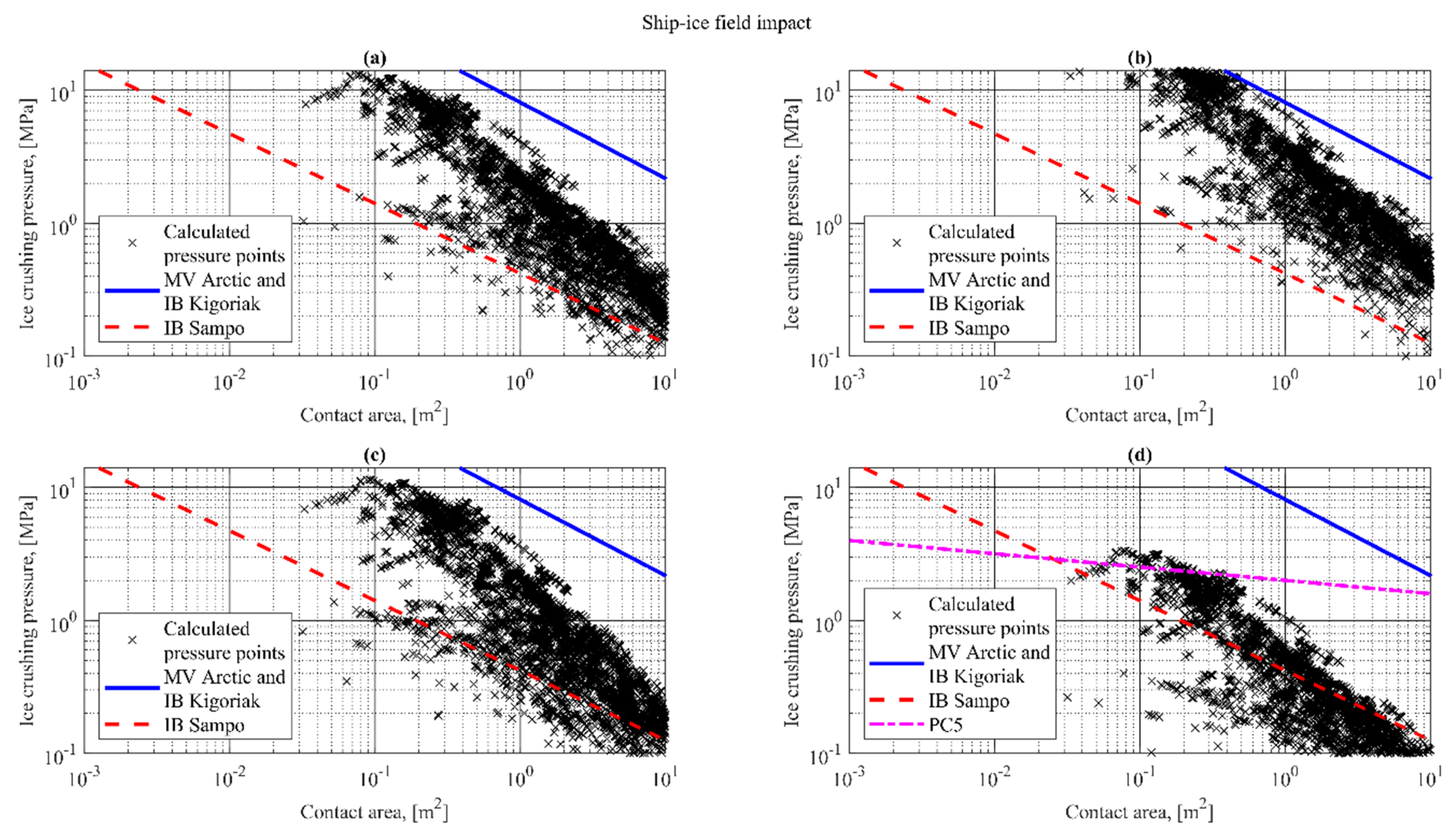
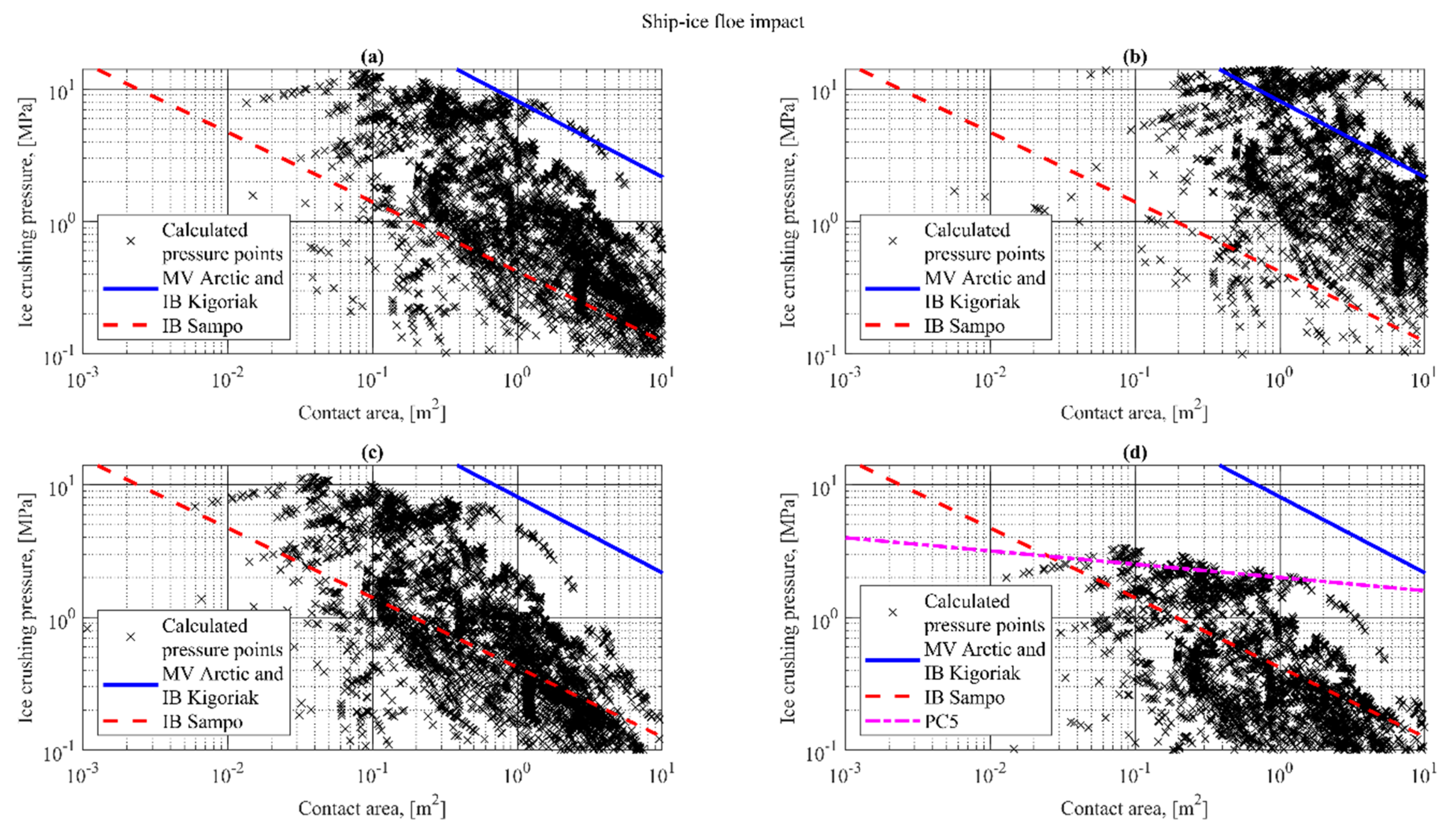
The considered full-scale ice load measurements (data set A–B) do not include any data to which we can compare our calculated values of ice crushing strength ${\sigma }_{cr}$. Thus, for the validation of our calculated ${\sigma }_{cr}$ values, we apply full-scale ice crushing pressure measurements conducted on MV Arctic and IB Kigoriak in Canadian waters, and on IB Sampo in the Baltic Sea [8]. We compare the calculated data points of ice crushing pressure (see Equation (10)) with the full-scale measurements as shown in Figure 9 and Figure 10.

Accordingly, we find that for different collision scenario assumptions, calculated ice crushing pressures $p$ values decrease with the size of the contact area. For both ship–ice field and ship–ice floe impacts, the best correlation with the measurements from the Baltic Sea (IB Sampo) and the Canadian waters (MV Arctic and IB Kigoriak) are obtained by applying angular- and round-contact geometries, respectively. We also find that the calculated pressure points tend to have a higher spread when calculated for an assumed ship–ice floe impact (Figure 10) than when calculated for an assumed ship–ice field impact (Figure 9). This is explained by the fact that in the case of ship–ice floe impacts, the ice load estimate depends on the ice floe size, which varies significantly as shown in Figure 3 and Figure 4.

We calculated the pressure-area points presented in Figure 9 and Figure 10 based on data set B. A similar analysis for data set A resulted in similar findings. It should be pointed out that Popov, et al. [9] do not specify any value of ice crushing pressure. The pressure-area relationship in accordance with PC5 is plotted in Figure 9d and Figure 10d. For comparison, in Figure 9d and Figure 10d we also plot the pressure-area relationship as determined in accordance with PC5. Because the PC rules only consider angular contact geometry, we do not plot any PC definition of ice crushing pressure for other contact geometries. As per Figure 9d and Figure 10d, we find that the slope of the PC5 pressure-area relationship is less steep than that of the pressure-area relationships determined based on full-scale measurements. Specifically, as indicated by the figures, the ice crushing pressures assumed by PC5 appear to be conservative for larger contact areas above approximately $5m^2$.

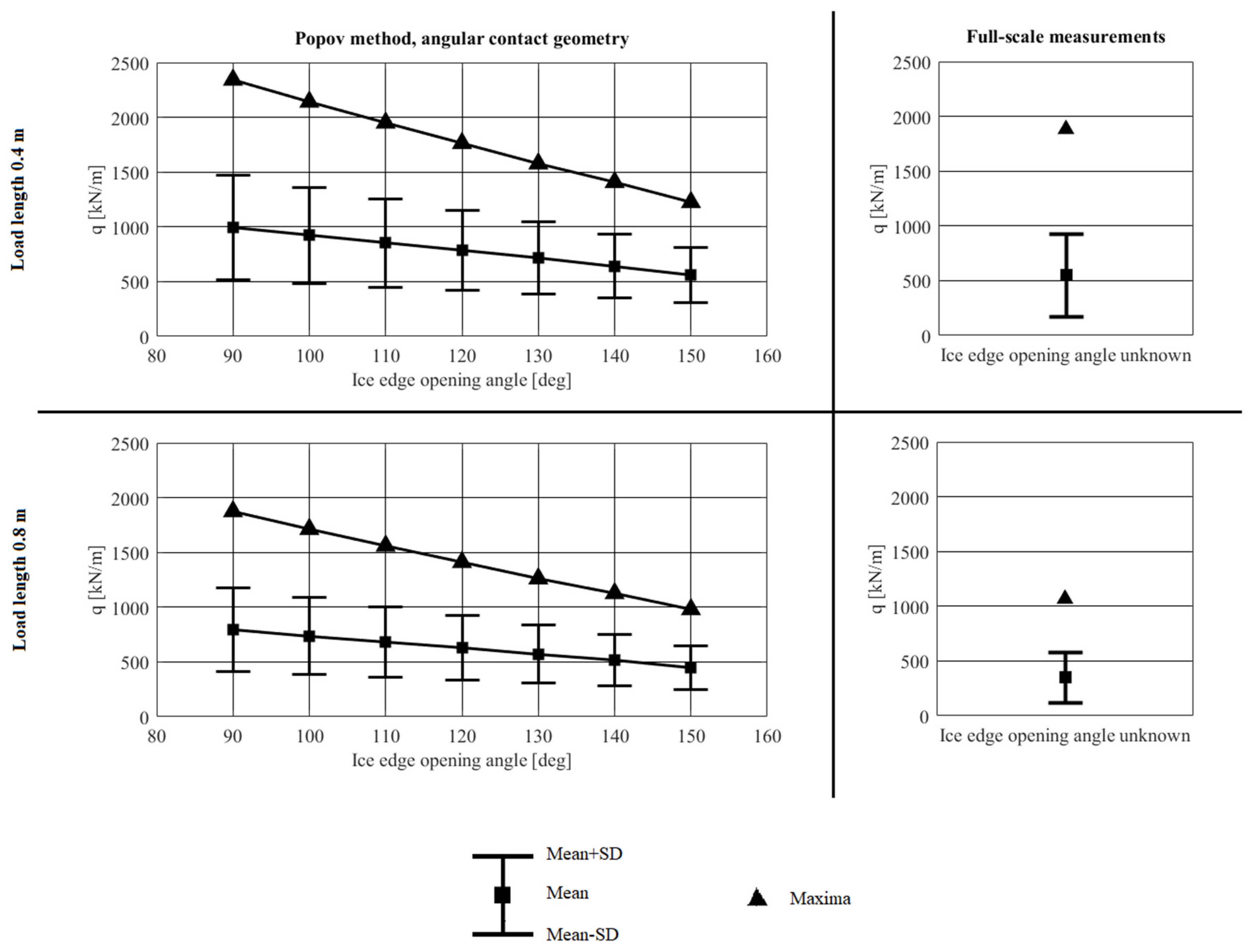
4.4. Influence of the Assumed Ice Edge Opening Angle

The PC design loads are calculated assuming an angular contact geometry with an ice edge opening angle ($\mathsf{\varphi }$) of 150°. To assess the influence of the assumed $\mathsf{\varphi }$-value, we calculated ice load estimates for $\mathsf{\varphi }$-values between 90°–150°. For the two different load lengths of 0.4 m and 0.8 m, Figure 11 shows how the calculated ice load ($q$), in terms of its mean, standard deviation and maximum, depends on the value of $\mathsf{\varphi }$, and how the calculated values compare to the measurements. We find that calculated ice load decreases with increasing ice edge opening angle ($\mathsf{\varphi }$) values. In addition, by comparing the calculated line loads with the measurements we find that:

• For one-frame spacing (load length = 0.4 m), a good agreement with the mean and maximum of the measurements is obtained for Φ-values around 150° and 110°, respectively.
• For two-frame spacing (load length = 0.8 m), a good agreement with the mean and maximum of the measurements is obtained for Φ-values around 150° and 140°, respectively.

5. Discussion and Conclusions

This study analyses a collision-energy-based method for the prediction of ice loading on ships known as the Popov Method. Even though the method is fundamentally analytical, due to unknowns related to the ship–ice interaction process and the material properties of sea ice, its practical application relies on numerous assumptions, some of which are empirically determined. To analyse the role of the assumptions, we compare ice load calculated for various assumptions with two different series of full-scale ice load measurements, referred to as data set A-B. Both of the data series originate from the same voyage, but differ in terms of operating conditions and modes. Data set A includes measurement data from operation in level and broken ice, including specific manoeuvres such as repeated ice ramming and reversing in ice. Data set B, on the other hand, mainly consists of measurement data from operation in broken and level ice without stops.

Towards addressing the research questions of Ch. 1, we calculate ice loads for two different types of collisions, namely the ship–ice floe and ship–ice field collisions. For each assumed collision type, we calculate loads for two different load length assumptions, namely 0.4 m and 0.8 m, and for four types of contact geometries, namely angular, right-apex oblique, round and symmetric v wedge.

In response to RQ1, we find that the obtained ice load prediction is very sensitive to assumptions concerning the modelling of the collision scenario and the operating conditions. For instance, depending on the assumed type of contact geometry, the obtained maximum load estimate might vary between 4%–122% of the corresponding full-scale measurement. This finding indicates that to get a reliable load estimate, the applied assumptions concerning the collision scenario and operating conditions (e.g., type of ice, floe size and ice thickness) must closely correspond to the actual condition.

In practice, this means that when applying the Popov Method, for instance in the context of goal-based design, multiple different ship–ice interaction scenarios must be considered to account for the often complex operating conditions of an Arctic ship.

In response to RQ2, we find that the best agreement with the full-scale measurements is obtained by applying the following combination of the assumptions: (a) Ship–ice floe collision, (b) angular contact geometry, and (c) load length of 0.4 m. Application of these assumptions overestimated the 10-min mean and extreme values of data set A by 33% and 32%, respectively. For data set B, on the other hand, the same assumptions underestimated the 10-min mean and extreme values by 1% and 36%, respectively. All other combinations of assumptions resulted in load estimates where either the mean or the extreme value deviated from either or both of the data series by more than 40%.

When applying an angular contact geometry, it is necessary to assume the value of the ice edge opening angle (ϕ). To investigate the role of this value, we calculated ice load estimates for ϕ-values between 90°–150°. We find that the calculated mean and extreme loads are negatively dependent on the ice edge opening angle. We conclude that the resulting underestimation of loads of data set B using the above defined preferred combination of assumptions could have been avoided by assuming an ice edge opening angle of around 110° instead of the applied value of 145°.

Assumptions behind the Popov Method and the related PC rules do not only concern the ship–ice interaction scenario, but also the material properties of ice, specifically the ice crushing strength. In this study, in order to enable a direct comparison between the calculated and measured loads, we estimate the ice crushing strength directly as a function of the ice salinity, brine volume, ice temperature, ice density and indentation rate. To validate the calculated ice crushing pressure values, we compare them with corresponding full-scale measurements. We find a good agreement between our calculated values and the corresponding measurements, both showing a negative relationship between ice crushing pressure and contact area.

As such, the present study does not aim to influence any existing regulations directly. However, by analysing the effects of the generalizing assumptions behind the PC rules, this work provides motivation and support for a goal-based design in line with the Polar Code. We believe that the present study contributes to a better understanding of the application of the Popov Method in design cases outside of the conditions formally considered in standard PC rules. For instance, to help to assess ice loading in pack ice in ship–ice floe interactions, or to assess ice loads on the aft or mid-body when specific contact geometries must be applied.

Because many of the actual ship–ice interaction parameters related to the measured ice loads, such as contact geometry and load length, are not fully known, the study cannot be considered a validation of the Popov Method. Nevertheless, it is promising that, for specific combinations of the assumptions, we obtained a good agreement with the measurements. Thus, we conclude that the Popov method has the potential to become a useful tool for goal-based design in the context of the Polar Code. It should be noted that this study is limited to assessing the effects of various assumptions when applying the Popov Method to estimate ice loading on ships. As such, it does not aim to directly compare PC design loads with full-scale measurements. Specifying a PC design load requires considering ice loads calculated for at least four sub-regions in the bow area along the waterline [38]. Because our applied full-scale data is limited to ice loads measured on two frames on the bow of the ship, it does not support a fair comparison. Therefore, comparing PC design loads with full-scale measurements remains a topic for future research. Another topic for future research is to address numerous unknowns related to the ship–ice interaction and sea-ice material properties, such as the actual ship–ice contact geometry and line load distribution in various types of ship–ice collisions.

References

- IMO. International Code for Ships Operating in Polar Waters (Polar Code); International Maritime Organization: London, UK, 2015. [Google Scholar]
- Kvålsvold, J. NSR Transit Shipping—A Risk Based Approach. In Northern Sea Route: New Opportunities; Det Norske Veritas: Moscow, Russia, 2012. [Google Scholar]
- IMO. Resolution MSC.386(94). Amendments of the International Convention for the Safety of Life at Sea, 1974, as Amended; International Maritime Organization: London, UK, 2014. [Google Scholar]
- IMO. Guidelines for the Approval of Alternatives and Equivalents as Provided for in Various IMO Instruments; International Maritime Organization: London, UK, 2013. [Google Scholar]
- IMO. Guidelines on Alternative Design and Arrangements for SOLAS Chapters II-1 and III. MSC.1/Circ.1212; International Maritime Organization: London, UK, 2006. [Google Scholar]
- IMO. Guidelines on Alternative Design and Arrangements for Fire Safety; MSC/Circ.1002; International Maritime Organization: London, UK, 2001. [Google Scholar]
- Daley, C. Oblique ice collision loads on ships based on energy methods. Ocean. Eng. Int. 2001, 5, 67–72. [Google Scholar]
- Kujala, P. Ice Loading on Ship Hull. In Encyclopedia of Maritime and Offshore Engineering; John Wiley & Sons: Hoboken, NJ, USA, 2017. [Google Scholar]
- Popov, Y.; Faddeyev, O.; Kheisin, D.; Yalovlev, A. Strength of Ships Sailing in Ice; Sudostroenie Publishing House: Leningrad, The Netherlands, 1967. [Google Scholar]
- Daley, C. Background Notes to Design Ice Loads; IACS Ad-hoc Group on Polar Class Ships, Transport Canada: Ottawa, ON, Canada; Memorial University: St. John’s, NL, Canada, 2000.
- Tunik, A. Dynamic Ice Loads on a Ship; International Association for Hydraulic Research: Hamburg, Germany, 1984. [Google Scholar]
- Kim, E.; Amdahl, J. Understanding the effect of the assumptions on shell plate thickness for Arctic ships. Trondheim. In Proceedings of the 23rd International Conference on Port and Ocean Engineering under Arctic Conditions, Trondheim, Norway, 14–18 June 2015; pp. 249–261. [Google Scholar]
- Huang, Y.; Qiu, W.; Ralph, F.; Fuglem, M. Improved Added Mass Modeling for Ship-Ice Interactions Based on Numerical Results and Analytical Models. In Proceedings of the Offshore Technology Conference, Houston, TX, USA, 5 May 2016. [Google Scholar]
- Dolny, J. Methodology for Defining Technical Safe Speeds for Light Ice-Strengthened Government Vessels Operating in Ice; Report No. SR—1475; The Ship Structure Committee: Washington, DC, USA, 2018. [Google Scholar]
- Storheim, M. Structural Response in Ship-Platform and Ship-Ice Collisions. Ph.D. Thesis, NTNU, Trondheim, Norway, January 2016. [Google Scholar]
- Kujala, P.; Goerlandt, F.; Way, B.; Smith, D.; Yang, M.; Khan, F.; Veitch, B. Review of risk-based design for ice-class ships. Mar. Struct. 2019, 63, 181–195. [Google Scholar] [CrossRef]
- Sazidy, M.; Daley, C.; Colbourne, B.; Wang, J. Effect of Ship Speed on Level Ice Edge Breaking. In Proceedings of the ASME 2014 33rd International Conference on Ocean, Offshore and Arctic Engineering, San Francisco, CA, USA; 2014. [Google Scholar]
- Daley R&E. Ice Impact Capability of DRDC Notional Destroyer; Defence Research and Development Canada: Halifax, NS, Canada, 2015.
- Daley, C.; Liu, J. Assesment of Ship Ice Loads in Pack Ice; ICETECH: Anchorage, AK, USA, 2010. [Google Scholar]
- Kendrick, A.; Quinton, B.; Daley, C. Scenario-Based Assessment of Risks to Ice Class Ships. In Proceedings of the Offshore Technology Conference, Houston, TX, USA, 4–7 May 2009. [Google Scholar]
- Quinton, B.; Daley, C. Realistic moving ice loads and ship structural response. In Proceedings of the 22nd International Offshore and Polar Engineering Conference, Rhodes, Greece, 17–22 June 2012. [Google Scholar]
- Quinton, B.; Daley, C.; Gagnon, R. Guidelines for the nonlinear finite element analysis of hull response to moving loads on ships and offshore structures. Ships Offshore Struct. 2017, 12, 109–114. [Google Scholar] [CrossRef]
- Liu, Z.; Amdahl, J. On multi-planar impact mechanics in ship collisions. Mar. Struct. 2018, 63, 364–383. [Google Scholar] [CrossRef]
- Croasdale, K. The limiting driving force approach to ice loads. In Proceedings of the Offshore Technology Conference, Houston, TX, USA, 7–9 May 1984. [Google Scholar]
- Enkvist, E.; Varsta, P.; Riska, K. The Ship-Ice Interecation; The International Conference on Port and Ocean Engineering under Arctic Conditions: Trondheim, Norway, 1979. [Google Scholar]
- Daley, K.; Riska, K. Review of Ship-ice Interaction Mechanics Report from Finnish-Canadian Joint Research Project No. 5 “Ship Interaction With Actual Ice Conditions” Interim Report on Task 1A; Report M-102; Ship Lab, Helsinki University of Technology: Espoo, Finland, 1990. [Google Scholar]
- Frederking, R. The Local Pressure-Area Relation in Ship Impact with Ice. In Proceedings of the 15th International Conference on Port and Ocean Engineering under Arctic Conditions, Helsinki, Finland, 23–27 August 1999. [Google Scholar]
- Masterson, D.; Frederking, R. Local contact pressures in ship/ice and structure/ice interactions. Cold Reg. Sci. Technol. 1993, 21, 169–185. [Google Scholar] [CrossRef]
- Croasdale, K.R. Crushing strength of Arctic ice. In Proceedings of the Coast and Shelf of the Beaufort Sea, Symposium, San Francisco, CA, USA, 7–9 January 1974. [Google Scholar]
- Riska, K. Ice edge failure process and modelling ice pressure. In Encyclopedia of Maritime and Offshore Engineering; John Wiley & Sons: Hoboken, NJ, USA, 2018. [Google Scholar]
- Michel, B.; Blanchet, D. Indentation of an S2 floating ice sheet in the brittle range. Ann. Glaciol. 1983, 4, 180–187. [Google Scholar] [CrossRef]
- Michel, B. Ice Mechanics; Laval University Press: Quebec, QC, Canada, 1978. [Google Scholar]
- Kheysin, D. Opredeleniye Vneshnikh Nagruzok Deystvuyushchikh na Korpus Sudna pri Ledovom Szhatii [Determination of External Loads Which Act on the Hull of A Ship When under Pressure from Ice]; Problemy Apktiki i Antapktiki: Leningrad, Russian, 1961; p. 7. [Google Scholar]
- Daley, C. Energy based ice collision forces. In Proceedings of the 15th International Conference on Port and Ocean Engineering under Arctic Conditions, Helsinki, Finland, 24–29 May 1999. [Google Scholar]
- Daley, C.; Kim, H. Ice collision forces considering structural deformation. In Proceedings of the ASME 2010 29th International Conference on Ocean, Offshore and Arctic Engineering, Shanghai, China, 6–11 June 2010; pp. 1–9. [Google Scholar]
- Li, F.; Kotilainen, M.; Goerlandt, F.; Kujala, P. An extended ice failure model to improve the fidelity of icebreaking pattern in numerical simulation of ship performance in level ice. Ocean Eng. 2019, 176, 169–183. [Google Scholar] [CrossRef]
- Daley, D.; Dolny, J.; Daley, K. Safe Speed Assessment of DRDC Notional Destroyer in Ice, Phase 2 of Ice Capability Assessment; Defence Research and Development Canada: Halifax, NS, Canada, 2017.
- IACS. Requirements Concerning POLAR CLASS; International Association of Classification Societies: London, UK, 2016. [Google Scholar]
- Kõrgesaar, M.; Kujala, P. Validation of the Preliminary Assessment Regarding the Operational Restrictions of Ships Ice-Strengthened in Accordance with the Finnish-Swedish Ice Classes When Sailing in Ice Conditions in Polar Waters; Aalto University publication series Science + Technology: Espoo, Finland, 2017. [Google Scholar]
- Suominen, M.; Kujala, P. The measured line load as a function of the load length in the Antarctic waters. In Proceedings of the 23rd International Conference on Port and Ocean Engineering under Arctic Conditions, Trondheim, Norway, 14–18 June 2015. [Google Scholar]
- Suominen, M.; Bekker, A.; Kujala, P.; Soal, K.; Lensu, M. Visual Antarctic Sea Ice Condition Observations during Austral Summers 2012–2016. In Proceedings of the 24 International Conference on Port and Ocean Engineering under Arctic Conditions, Busan, Korea, 11–16 June 2017. [Google Scholar]
- Idrissova, S.; Kujala, P.; Repin, R.; Li, F. The study of the Popov method for estimation of ice loads on ship’s hull using full-scale data from the Antarctic sea. In Proceedings of the 25th International conference on Port and Ocean Engineering under Arctic Conditions, Delft, The Netherlands, 9–13 June 2019. [Google Scholar]
- Suominen, M.; Su, B.; Kujala, P.; Moan, T. Comparison of measured and simulated short term ice loads on ship hull. In Proceedings of the 22nd International Conference on Port and Ocean Engineering under Arctic Conditions, Espoo, Finland, 9–13 June 2013. [Google Scholar]
Figure 1.
Considered contact geometry models: (a) Round; (b) Angular; (c) Symmetric v wedge; (d) Right-apex oblique; (e) Spherical; (f) Pyramid (Adapted with permission from Daley [34], International Conference on Port and Ocean Engineering under Arctic Conditions, 1999, and from Daley & Kim [35], The American Society of Mechanical Engineers, 2010).
Figure 2.
Location of strain gauges on the S.A. Agulhas II. (The figure was determined based on Suominen & Kujala [40]).
Figure 3.
Extract from data set A, showing how the measured ice floe diameter, ice thickness and speed vary during a selected period of 14 h.
Figure 4.
Extract from data set B, showing how the measured ice floe diameter, ice thickness and speed vary during a selected period of 8 h.
Figure 5.
Excerpt of the measured and calculated line ice loads for data set A.
Figure 6.
Comparison between loads calculated for different collision scenario assumptions with corresponding full-scale measurements in terms of 10-min mean, standard deviation (SD) and maximum. Load length corresponds to loads on one frame spacing (frame 134), whereas load length corresponds to loads on two frame spacing (frame 134 + 134.5).
Figure 7.
Measured and estimated line loads from ship–ice floe impact for data set B.
Figure 8.
Comparison of measured line loads with estimated by Popov Method for data set B.
Figure 9.
Measured vs. calculated ice crushing pressure-area relationships. Collison type: Ship–ice field impact. Contact geometries: (a) Right-apex oblique; (b) Round; (c) Symmetric v wedge; (d) Angular. The ice crushing pressure-area relationships determined based on measurements conducted on MV Arctic and IB Kigoriak, and on IB Sampo, were determined based on Kujala [8].
Figure 10.
Measured vs. calculated ice crushing pressure-area relationships. Collison type: Ship–ice floe impact. Contact geometries: (a) Right-apex oblique; (b) Round; (c) Symmetric v wedge; (d) Angular. The ice crushing pressure-area relationships determined based on measurements conducted on MV Arctic and IB Kigoriak, and on IB Sampo, were determined based on Kujala [8].
Figure 11.
Comparison of line loads from the Popov Method for different ice edge opening angles of angular contact geometry.