Formation Control and Distributed Goal Assignment for Multi-Agent Non-Holonomic Systems


Institute of Automation and Robotics, Poznań University of Technology (PUT), Piotrowo 3A, 60-965 Poznań, Poland
Appl. Sci. 2019, 9(7), 1311; https://0-doi-org.brum.beds.ac.uk/10.3390/app9071311
Submission received: 5 March 2019
/
Revised: 24 March 2019
/
Accepted: 25 March 2019
/
Published: 29 March 2019
(This article belongs to the Special Issue Advanced Mobile Robotics)
Abstract
:This paper presents control algorithms for multiple non-holonomic mobile robots moving in formation. Trajectory tracking based on linear feedback control is combined with inter-agent collision avoidance. Artificial potential functions (APF) are used to generate a repulsive component of the control. Stability analysis is based on a Lyapunov-like function. Then the presented method is extended to include a goal exchange algorithm that makes the convergence of the formation much more rapid and, in addition, reduces the number of collision avoidance interactions. The extended method is theoretically justified using a Lyapunov-like function. The controller is discontinuous but the set of discontinuity points is of zero measure. The novelty of the proposed method lies in integration of the closed-loop control for non-holonomic mobile robots with the distributed goal assignment, which is usually regarded in the literature as part of trajectory planning problem. A Lyapunov-like function joins both trajectory tracking and goal assignment analyses. It is shown that distributed goal exchange supports stability of the closed-loop control system. Moreover, robots are equipped with a reactive collision avoidance mechanism, which often does not exist in the known algorithms. The effectiveness of the presented method is illustrated by numerical simulations carried out on the large formation of robots.
1. Introduction
The idea to use artificial potential fields to control manipulators and mobile robots was introduced by Khatib [1] in 1986. In this approach both attraction to the goal and repulsion from the obstacles are negated gradients of the artificial potential functions (APF). His paper not only presents the theory, but also a solution of the practical problem, implemented in the Puma 560 robot simulator. It is worth noting that much earlier, in 1977, Laitmann and Skowronski [2] investigated control of two agents avoiding collision with each other. This work was purely theoretical. The authors continued their work in the following years [3].
Since the 1990s, intensive research on the trajectory tracking control for non-holonomic mobile robots has been conducted [4,5,6]. The algorithm presented further in this paper is based on the method from [4]. This method considers a single, differentially-driven mobile robot moving in a free space. Its goal is to track a desired trajectory. The paper includes a stability analysis.
The last decade has seen a lot of publications on multiple mobile robot control. In [7], the goal of multiple mobile robots is to track desired trajectories avoiding inter-agent collisions. The same type of task is considered further in this paper. The tracking controller is different, as is the formula of APF, but the method of combining trajectory tracking and collision avoidance is the same. In [8], the same type of task is considered, but the dynamics of mobile platforms and uncertainties of its parameters are taken into account. Kowalczyk et al. [9] propose a vector-field-orientation algorithm for multiple mobile robots moving in the environment with circle shaped static obstacles. The dynamic properties of mobile platforms are also taken into account. The paper [10] presents a kinematic controller for the formation of robots that move in a queue. The goal is to keep desired displacements between robots and avoid collisions in the transient states. Hatanaka et al. [11] investigate a cooperative estimation problem for visual sensor networks based on multi-agent optimization techniques. The paper [12] addresses the formation control problem for fleets of autonomous underwater vehicles. Yoshioka et al. [13] deal with formation control strategies based on virtual structure for multiple non-holonomic systems.
Recent years have also seen a number of publications on barrier functions. In [14], coordination control for a group of mobile robots is combined with collision avoidance provided by a safety barrier. If the coordination control command leads to collision, the safety barrier dominates the controller and computes a safe control closest to coordination control law. In the method proposed in [15] control barrier functions are unified with performance objectives expressed as control Lyapunov functions. The authors of the paper [16] provide a theoretical framework to synthesize controllers using finite time convergence control barrier functions guided by linear temporal logic specifications for continuous time multi-agent systems.
The paper [17] addresses the problem of optimal goal assignment for the formation of holonomic robots moving on a plane. A linear bottleneck assignment problem solution is used to minimize the maximum completion time or maximum distance for any robot in the formation. The authors of [18] consider formation of non-holonomic mobile vehicles that has to change the geometrical shape of the formation. Goal assignment minimizes the total distance travelled by agents. The exemplary application indicated by the authors is reconfiguration of the formation when it approaches a narrow passage. In [19,20], goal assignment based on distances squared is proposed and tested for large formations, but the collision avoidance is resolved at the trajectory planning level. This makes this approach less robust in the case of unpredictable disturbances (which are natural in real applications). The second of these papers proposes a solution to the problem of collision avoidance with static and dynamic obstacles present in the environment. In [21], collision avoidance is obtained by applying safety constraints in optimal trajectory generation. The robots do not have non-holonomic constraints (they are quadrotors) and they have to change the shape of the formation using goal assignment that minimizes the total distance travelled by the robots. Turpin et al. [22] present concurrent assignment and planning of trajectories (CAPT) algorithms. The authors propose two variations of the algorithm: centralized and decentralized, and test them on a group of holonomic mobile robots moving in a three-dimensional space. The solution is based on the Hungarian assignment algorithm. The above-mentioned works do not deal with the problem of closed-loop control. For this reason stability issues were not considered there.
In comparison to the above two approaches, here the user or the higher level controller determines the locations of desired trajectories according to the needs (this can be considered as an expected feature in many applications). In addition, trajectory generation is decoupled from the closed-loop control (the system is modular). Such a solution is considered as a design pattern in robotics. The algorithm is responsible for tracking these trajectories and reacting to the risk of collisions between agents at the same time. Even if initial states of individual robots are far from the desired ones, the collision avoidance module works correctly. Furthermore, the algorithm characterizes conceptual and computational simplicity. The paper considers preserving data integrity during the goal exchange as it requires a simultaneous change of states in remote systems. This subject is omitted in the literature on goal assignment in multi-robot systems. To the best of the author’s knowledge, no work has been published so far that proposes closed-loop control for multiple non-holonomic mobile robots combined with target assignment with analysis based on a Lyapunov-like function for both the tracking algorithm and target assignment. Panagou et al. [23] propose a similar method, but it assumes that agents are fully-actuated (modeled using integrators), and the analysis is based on multiple Lyapunov-like functions. This algorithm also uses a different criterion for goal exchange.
The algorithm proposed in this paper is applicable mainly to the homogeneous formations of non-holonomic mobile robots but also in the scenarios when two or more robots of the same type are involved in task execution. For a high number of applications of multiple mobile robots this situation occurs, e.g., exploration, mapping, safety, and surveillance.
In Section 2 a control algorithm for the formation of non-holonomic mobile robots is described. Section 3 analysis stability. The simulation results are presented in Section 4. The goal exchange algorithm is introduced in Section 5. Section 6 provides stability analysis of extended algorithm. Section 7 details distributed implementation. Some generalization of the proposed goal exchange rule is given in Section 8. Section 9 discusses the problem of maintaining data integrity in the process of the goal exchange. Section 10 offers simulation results for the goal exchange algorithm. Section 11 presents simulation results for limited wheel velocity controls. In the last Section concluding remarks are provided.
2. Control Algorithm
The kinematic model of the i-th differentially-driven mobile robot (, N—number of robots) is given by the following equation:
where vector denotes the pose and , , are the position coordinates and orientation of the robot with respect to a global, fixed coordinate frame. Vector is the control vector with denoting the linear velocity and denoting the angular velocity of the platform.
The task of the formation is to follow the virtual leader that moves with desired linear and angular velocities . The robots are expected to imitate the motion of the virtual leader. They should have the same velocities as the virtual leader. The position coordinates of the virtual leader are used as a reference position for the individual robots but each of them has different displacement with respect to the leader:
where is desired displacement of the i-th robot. As the robots position converge to the desired values their orientations converge to the orientation of the virtual leader .
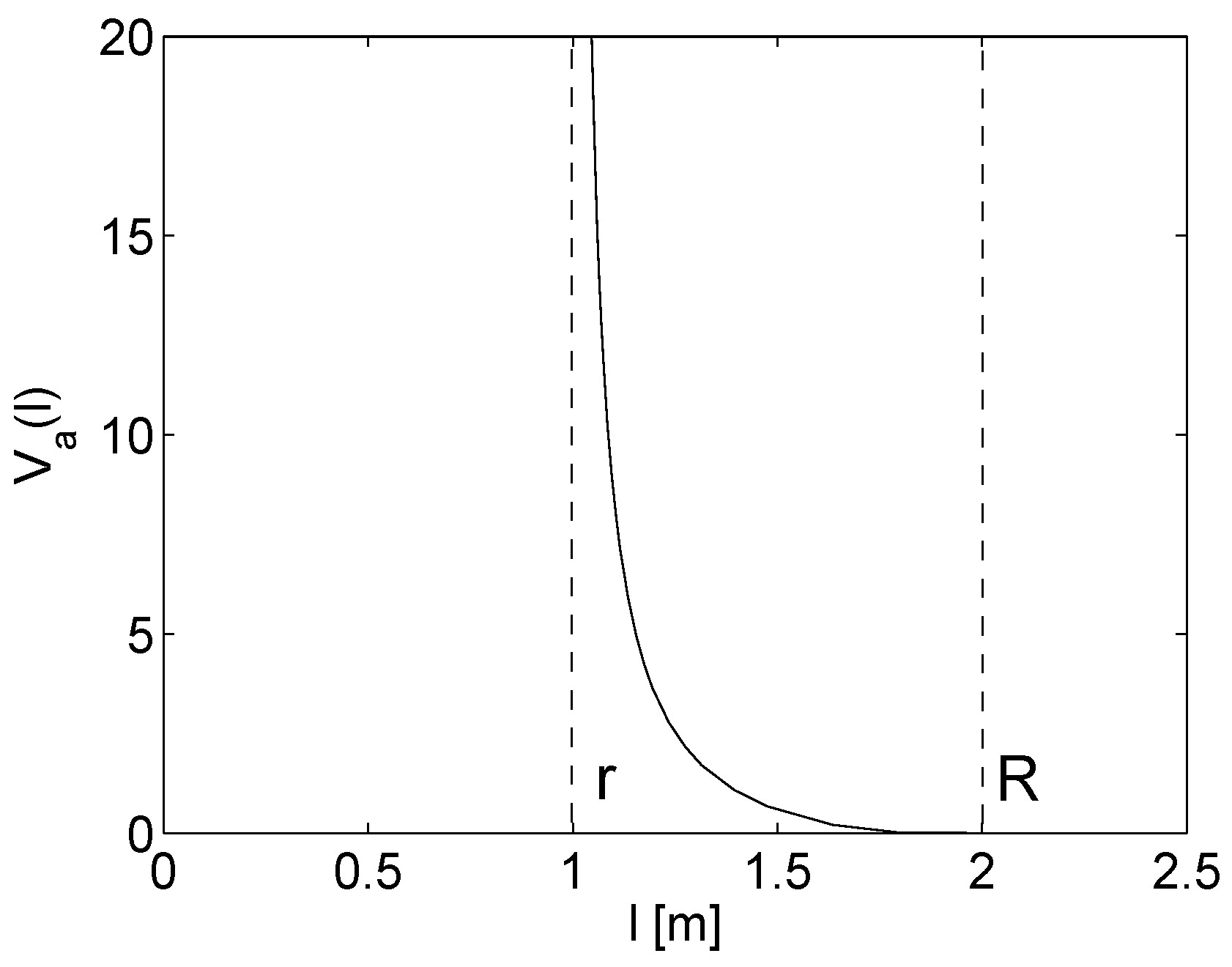
The collision avoidance behaviour is based on the APF. This concept was originally proposed in [1]. All robots are surrounded by APFs that raise to infinity near objects border (j—number of the robots/obstacles) and decreases to zero at some distance , .
One can introduce the following function [6]:
that gives output . The distance between the i-th robot and the j-th robot is defined as the Euclidean length .
Scaling the function given by Equation (3) within the range can be given as follows:
that is used later to avoid collisions.
In further description, the terms ‘collision area’ or ‘collision region’ are used for locations fulfilling the condition . The range is called ‘collision avoidance area’ or ‘collision avoidance region’ (Figure 1).
The goal of the control is to drive the formation along the desired trajectory avoiding collisions between agents. It is equivalent to bringing the following quantities to zero:
Assumption 1.
.
Assumption 2.
If robot i gets into the collision avoidance region of any other robot j, its desired trajectory is temporarily frozen (, ). If the robot leaves the avoidance area its desired coordinates are immediately updated. As long as the robot remains in the avoidance region, its desired coordinates are periodically updated at certain discrete instants of time. The time period of this update process is relatively large in comparison to the main control loop sample time.
Assumption 1 comes down to the statement that desired paths of individual robots are planned in such a way that in steady state all robots are out of the collision avoidance regions of other robots.
Assumption 2 means that the tracking process is temporarily suspended because collision avoidance has a higher priority. Once the robot is outside the collision detection region, it updates the reference to the new values. In addition, when the robot is in the collision avoidance region its reference is periodically updated. This low-frequency process supports leaving the unstable equilibrium points that occur e.g., when one robot is located exactly between the other robots and its goal.
The system error expressed with respect to the coordinate frame fixed to the robot is described below:
Using the above equations and non-holonomic constraint the error dynamics between the leader and the follower are as follows:
One can introduce the position correction variables that consist of position error and collision avoidance terms:
depends on and according to Equation (5). It is assumed that the robots avoid collisions with each other and there are no other obstacles in the taskspace. The correction variables can be transformed to the local coordinate frame fixed in the mass centre of the robot:
Differentiating the first two equations of (5) with respect to the and respectively one obtains:
Using (10) one can write:
Taking into account Equations (8) and (9) the gradient of the APF can be expressed with respect to the local coordinate frame fixed to the i-th robot:
Equation (12) can be verified easily by taking partial derivatives of with respect to , and taking into account the inverse transformation of the first two equations of Equation (6).
Using Equation (11), the above equation can be written as follows:
Equations (9) and (12) can be transformed to the following form:
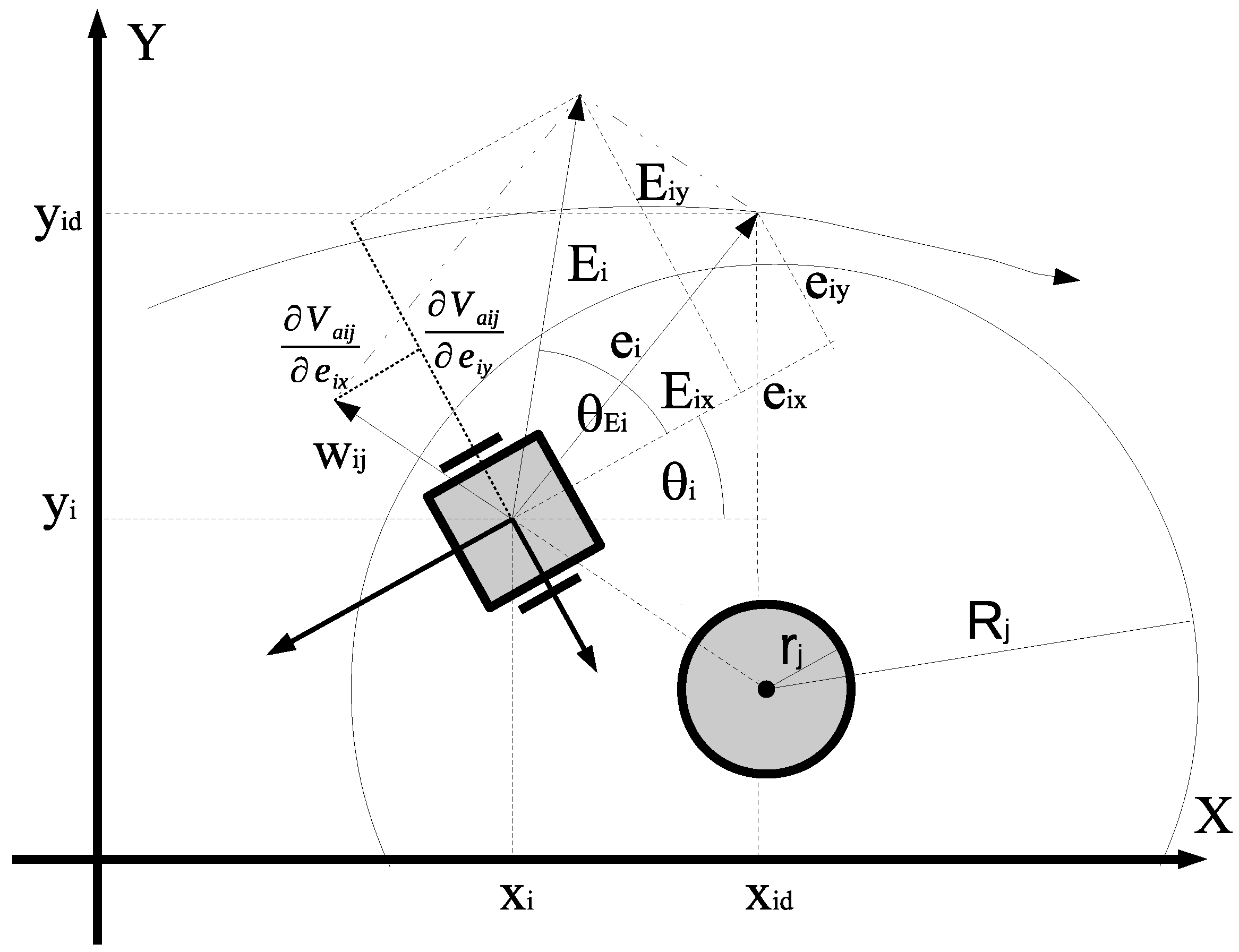
where each derivative of the APF is transformed from the global coordinate frame to the local coordinate frame fixed to the robot. Finally, the correction variables expressed with respect to the local coordinate frame (Figure 2) are as follows:
The trajectory tracking algorithm from [4] was chosen based on the author’s experience. It is simple, easy to implement, and, above all, it is effective. Tracking control with persistent excitation [24] and the vector-field-orientation method [25] were also taken into account. The former gives much worse convergence time, the latter gives even better convergence but it is more difficult to implement on a real robot.
The control for N robots extended by the collision avoidance is as follows:
where , and are positive constant design parameters.
Assumption 3.
If the value of the linear control signal is less than considered threshold value , i.e., (-positive constant), it is replaced with a new value , where
(indexes omitted for simplicity).
Transforming (18) using (16) and taking into account Assumption 2 (when the robot gets into the collision avoidance region, in the collision avoidance state, velocities and are replaced with 0 value) error dynamics can be expressed in the following form:
Orientation error decreases exponentially to zero (refer to the last equation in (19)).
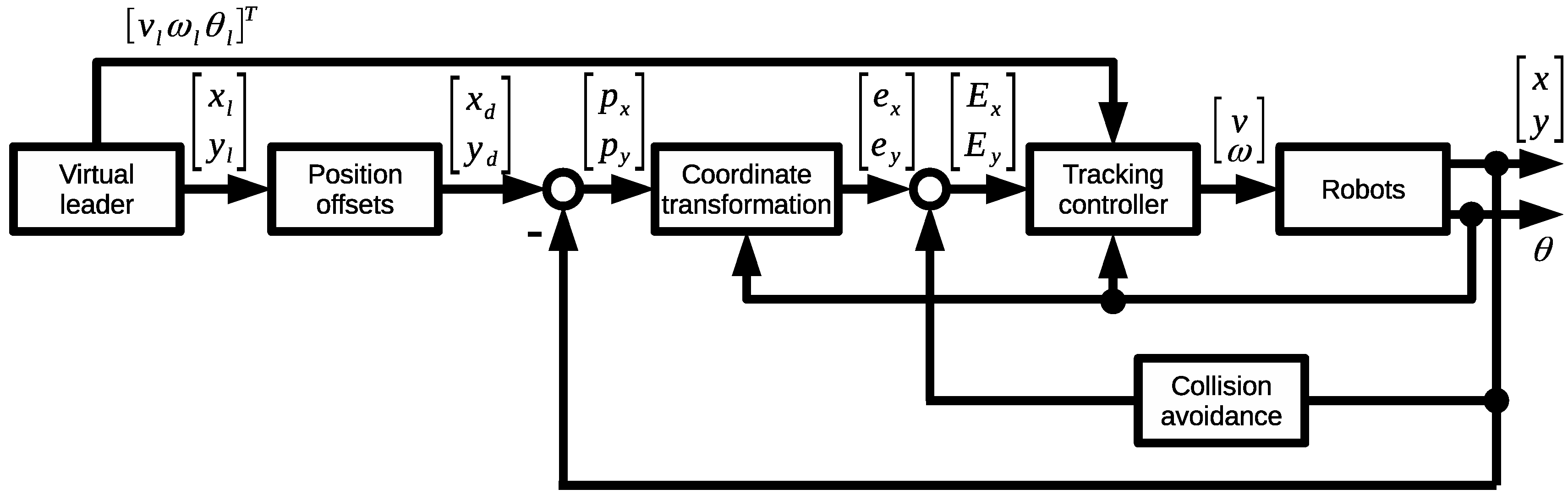
In Figure 3 a schematic diagram of the control system is presented. The following signal vectors are marked: , , , , , , .
3. Stability of the System
In this section stability analysis of the closed-loop system is presented. When the i-th robot is out of the collision regions of the other robots (APF takes the value zero) the analysis given in [4] is actual and will not be repeated here. Further the analysis for the situation in which the i-th robot is in the collision region of other robot is presented.
For further analysis a new variable is introduced: ( is a version of the function covering all four quarters of the Euclidean plane)—auxiliary orientation variable.
Proposition 1.
As stated in [7], if (the combination of obstacle position and reference trajectory drive the robot into the neighbourhood of a singular configuration where the condition in Proposition 1 does not hold) one solution is to add perturbation to the desired signal. The system can also leave the neighbourhood of the singularity easily since the robot can reorient itself in place if the condition is not satisfied. This requires a special procedure to be implemented, which will not be discussed here.
Proof.
Consider the following Lyapunov-like function:
When the robot is outside of the collision avoidance region, i.e., , the system is equivalent to the one presented in [4] (robot moving in a free space) and stability analysis presented in this paper still holds.
If the robot is in the collision avoidance region of the other robot time derivative of the Lyapunov-like function is calculated as follows:
Taking into account Equation (15) the above formula can be transformed to the following form:
Next, using Equation (19) one obtains:
Substituting and , in the above equation one obtains:
To simplify further calculations, new scalar functions are introduced:
Taking into account (24) can be written as follows:
The closed-loop system is stable () if the following condition is fulfilled:
As because of the assumption in Proposition 1 it cannot be arbitrarily small, the condition (27) can be met by setting a sufficiently high value of or by reducing .
Note that the error dynamics (19) with frozen reference velocities can be decomposed into two subsystems (Figure 4). The origin of the system is exponentially stable if . Each of the subsystems is input to state stable (ISS). Stability of the origin may be concluded invoking the small-gain theorem for ISS systems [26].
The boundedness of the output of the collision avoidance subsystem is necessary to prove stability. Taking the first equation in (19), one can state that if is sufficiently high (that happens if the robot is very close to the obstacle; there is no problem of boundedness in the other cases (refer to the properties of the APF, Figure 1)), i.e., , , and the error dynamics can be approximated as follows:
From the Equation (28) it is clear that and have different signs and as a result . To fulfil the condition that is less than zero the second term on the right hand side must be less than the first one taking their absolute values. This can be obtained by reducing parameter (refer to Equation (16)). The property guarantees boundedness of both and . Finally one can state that the collision avoidance block that is input to the system shown in Figure 4 also has bounded output and both error components and in are bounded.
The above is true if the robot is not located close to the boundary of more than one robot at a time. This situation is unlikely because it leads to high controls that increase the distance between the robots quickly and therefore this will not be considered further. □
As shown in [7] collision avoidance is guaranteed if and , .
Each robot needs information about positions of other robots in its neighbourhood to avoid collision (their orientations are not needed). It can be obtained using on-board sensors with the range equal to or greater than R. In addition, robots need to know their position and orientation errors to calculate the tracking component of the control. This requirement imposes the use of a system allowing localization with respect to the global coordinate frame, because usually, the motion task is defined with respect to it. The author plans to conduct experiments on real robots in the near future. The OptiTrack motion capture system will be used to obtain coordinates of robots (positions and orientations) which is enough for control purposes.
4. Simulation Results
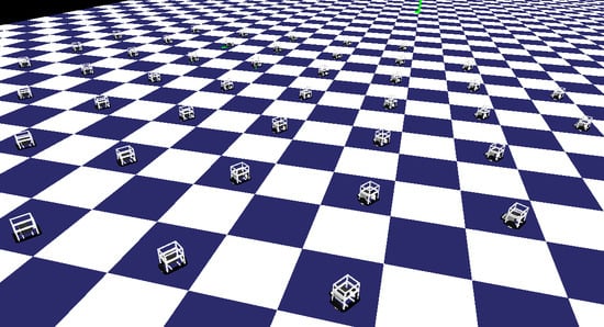
In this section a numerical simulation for a group of mobile robots is presented. The initial coordinates (both positions and orientations) were random. The goal of the formation was to follow a circular reference trajectory at the same time avoiding collisions between agents. The formation had a shape of a circle. The assignments of robots to particular goal points were also random.
The following settings of the algorithm were used: , , , , , .
Figure 5a shows paths of robots on the plane. To make the presentation clearer in Figure 5a–g signals of 45 robots are grey while the 3 selected ones are highlighted in black. In Figure 5h the three selected inter-agent distances are highlighted in black. Figure 5b,c present graphs of x and y coordinates as a function of time. The robots converged to the desired values in 115 s. Figure 5d shows a time graph of the orientations. In Figure 5e,f linear and angular controls, respectively, are shown. Initially and in the transient state, their values were high, exceeding the maximum values of a typical mobile platform. In practical implementation, they should be scaled down to realizable values. Figure 5g presents a time graph of the freeze procedure (refer to Assumption 2) of all robots. Although the drawings are not easily readable (because they include the ‘freeze’ signal of all robots), one can interpret that the last collision avoidance interaction ends in . In Figure 5h relative distances between robots are shown. Important information that can be read from this drawing is that no pair of robots reaches the inter-agent distance lower than or equal to (dashed line). This means that no collision has occurred.
5. Goal Exchange
This section presents a new control that introduces the ability to exchange goal between agents.
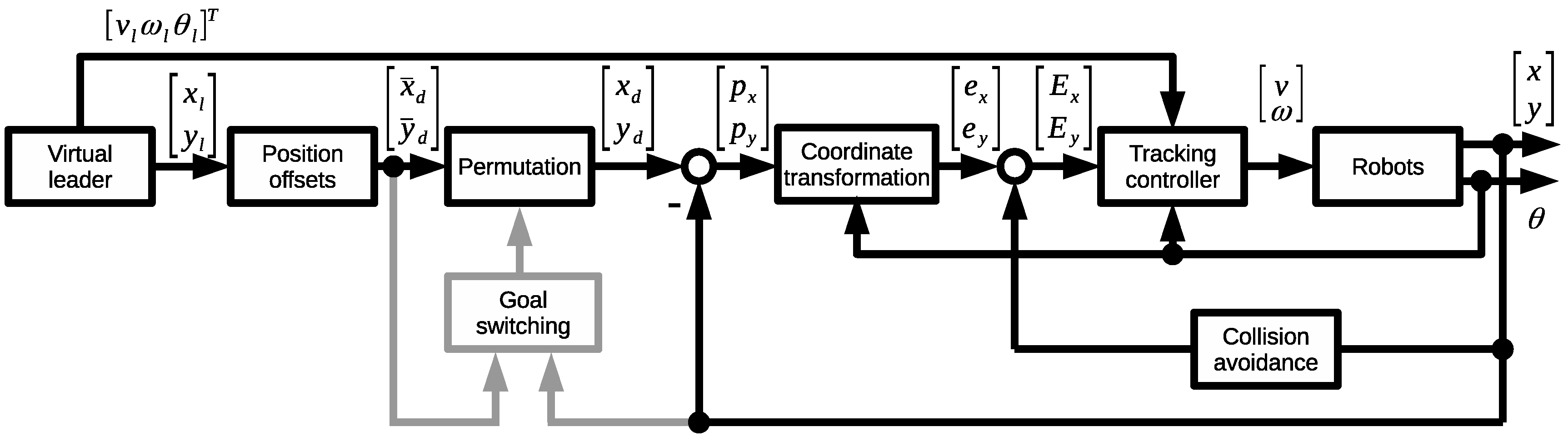
The block diagram of the new control is shown in Figure 6. Two new blocks are included: goal switching and permutation block.
In the method proposed here Equation (2) is replaced as follows:
The new variables and are not representing the goal position of robot i, but the goal that can be assigned to any robot in the formation.
One can introduce the following aggregated goal coordinate vectors: and (numbers in lower index represent the numbers of the goals). The assignment of goals to particular robots is computed using permutation matrix :
Resulting vectors contained goal coordinates assigned to particular robots and (number in lower index represents the number of the robot).
An additional control loop is introduced that acts asynchronously to the main control loop (Figure 6).
Let’s assume that at some instant of time an arbitrary goal m is assigned to the robot k and another goal n is assigned to the robot l. This can be written as:
There are ones in permutation matrix at element and and all other elements in rows m, n and columns k, l were zero.
At some discrete instant in time for the pair of robots k and l and their goals m and n the following switching function was computed:
where .
If the switching function takes the value of 1 matrix P is changed as follows:
where is the permutation matrix before switching.
The elementary matrix is a row-switching transformation. It swaps row m with row n and it takes the following form:
Transformation (33) describes a process of the goal exchange between agents k and l at time . After that goal m, was assigned to robot l and goal n was assigned to robot k that is equivalent to the following equalities:
Note that the process of goal exchange is asynchronous with the main control loop. It operated at lower frequency because it required communication between remote agents, which is time consuming. The low frequency subsystem is highlighted in grey in Figure 6.
6. Stability of the System with Target Assignment
The goal exchange procedure significantly improves system convergence and reduces the number of collision avoidance interactions between agents. On the other hand, its execution time was not critical for the control of the system.
Stability analysis of the control system with goal switching was conducted using the same Lyapunov-like function (20) as in Section 3.
Proposition 2.
The procedure given by Equation (33) results in a decrease of the Lyapunov-like function Equation (20).
Proof.
A hypothetical position error can be expressed in a local coordinate frame by the following transformation
that is invariant under scaling, and thus, the following equality holds true:
(notice that index i is the number of the goal and index j is the number of the robot).
Using Equation (37) the switching function (32) can be rewritten as follows:
To carry out further analysis the Lyapunov-like function (20) will be rewritten as follows:
Terms and are related to the position errors of robot k and l, respectively. Notice that other terms of the Lyapunov-like function V are invariant under goal assignment as depends only on the distances between agents and remains constant because all agents share the same reference orientation . The position error terms related to robots that were not involved in goal exchange were also invariant under goal exchange.
Two cases will be considered further: case 1 at , and case 2 at .
In case 1 the sum of position terms of robots k and l can be transformed using (36) and (31) as follows:
In case 2 the sum of position terms of robot k and l, repeating the initial steps above and taking into account (35) is given by:
Note that (omitting the constant multiplier ) is the left hand side of the inequality in the first condition of the switching function (32) while is the right hand side of this condition (also omitting the multiplier). This leads to the conclusion that as , goal exchange results in a rapid decrease (discontinuous) of the Lyapunov-like function. □
All other properties of the V still hold including if the condition given by Equation (27) is fulfilled.
Proposition 3.
The procedure given by Equation (33) results in a decrease of the sum of the position errors squared.
Proof.
As and in Equation (39) are invariant under the goal assignment and the sum of all other terms represent the sum of the position errors squared (omitting the constant multiplier ), the proof of Proposition 3 comes directly from Proposition 2. □
Notice that the sum of the position errors squared can be easily expressed in the global coordinate frame using equality (refer to Equation (6)) to transform the position error of each robot in (39).
The tracking algorithm presented in Section 2 together with the goal exchange procedure resulted in time intervals continuous algorithm with discrete optimization that uses the Lyapunov-like function as a criterion to be minimized. The discontinuities occur in two situations: when the robot is in the collision avoidance region (the reference trajectory is temporarily frozen and then unfrozen) and when a pair of agents exchange the goals. The set of these discontinuity points was of zero measure. Note that including goal exchange in the control reinforces fulfilling condition (27) because it supports reduction of the component .
The presented algorithm does not guarantee optimal solutions but each goal exchange improves the quality of the resulting motion. The total improvement depends significantly on the initial state of the system. In extreme cases, there is a situation in which the initial coordinates are close to optimal. The procedure may lead to no goal exchange, and thus no improvement, even though communication costs have been incurred. On the other hand, if the initial coordinates are not special, benefits of using the procedure are usually considerable.
7. Distributed Goal Exchange
The procedure described in Section 5 can be implemented in a distributed manner. Both key components of the goal switching algorithm; computation of the switching function (32) and permutation matrix transformation (33), involve only two agents. Reliable connection between them was needed as the process was conducted in a sequence of steps. After the agents establish the connection one of them (i-th) sends its position coordinates and goal location to the other (j-th). The second robot computes switching function (32) which is the verdict on the goal exchange. If it is negative the robots disconnect and continue motion to their goals, otherwise robot j sends its position coordinates and goal location to robot i. This part is critical in the process and must be designed carefully to ensure correct task execution.
To make distributed goal exchange possible, the robots must be equipped with the on-board radio modules allowing inter-agent communication. Even if not all pairs of agents were capable of communicating, the goal exchange algorithm improved the result. On the other hand, without communication between all pairs of agents the algorithm did not fail. In the vast majority of environments there was no problem with the communication range (current technology allows communication through many routers, base stations and peers). The exceptions may be space and oceanic applications. They will not be considered here. The author plans to conduct laboratory experiments where there are no restrictions on communication. From the practical point of view, robots need to know the network addresses of other robots and sequentially attempt to establish connection and, if successful, exchange the goals.
8. On Some Generalization
The condition (32) can be rewritten in more general form as follows:
Taking leads to the shortest path criterion that seems to be natural in many cases because the shortest path induces lower motion cost. Unfortunately this observation may not be true in a cluttered case. This will be shown later in this section. Note that in the cases for the Lyapunov analysis is much more complex. In [23] the similar method that results in the shortest total distance to the goals is presented.
Several specific scenarios for the simple case of two robots are analysed further. These scenarios should be treated as an approximation of a real case because typically paths of real robots are not straight lines in the case of the platforms that are not fully actuated (like the differentially driven mobile platform considered here).
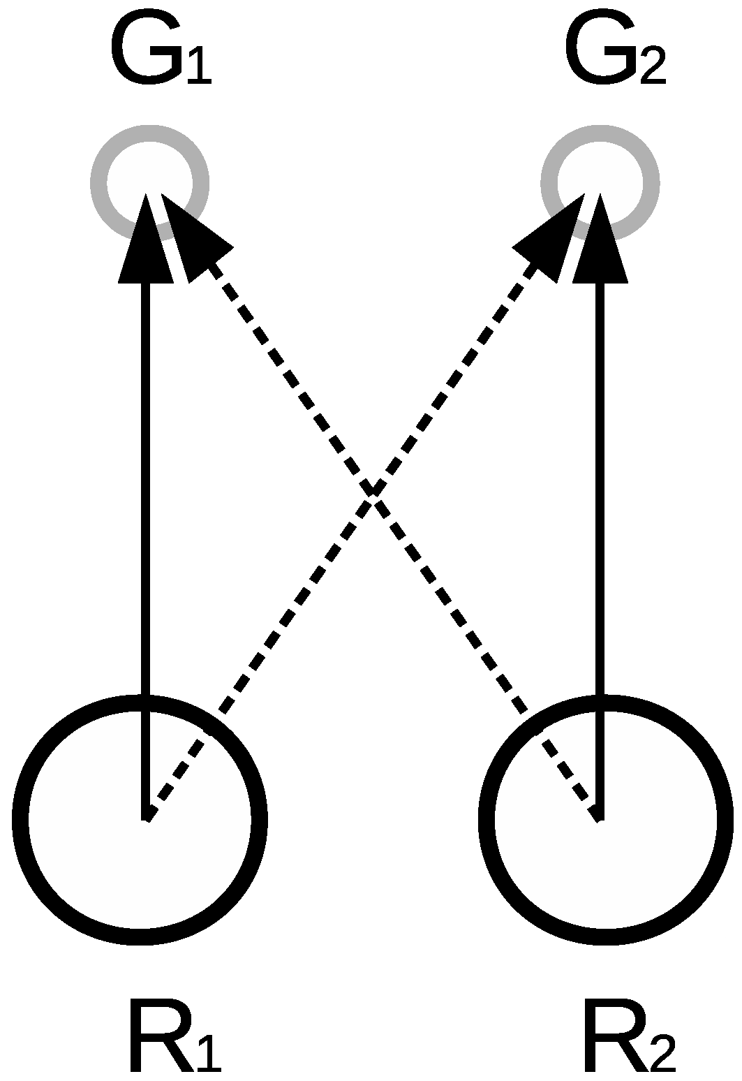
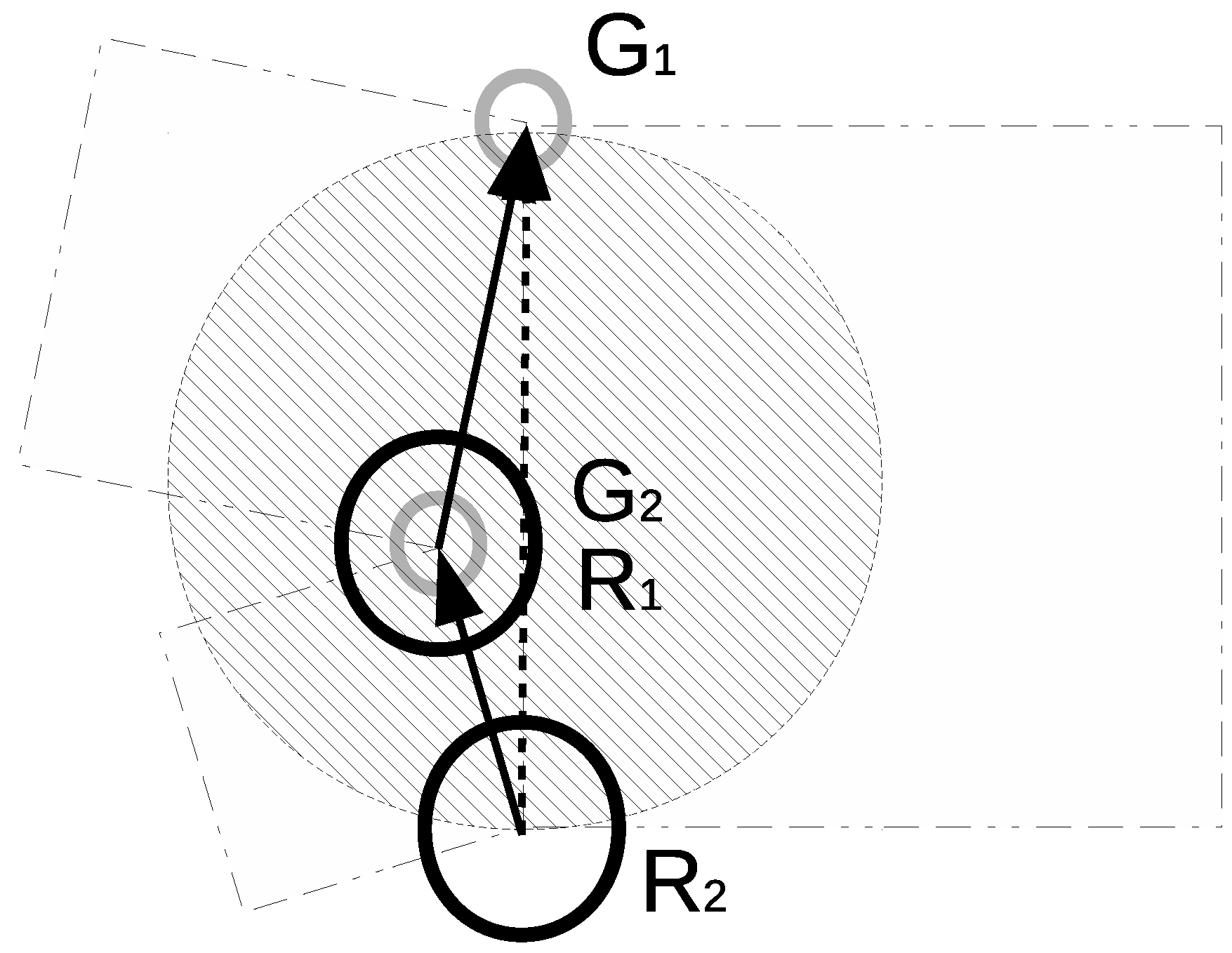
In Figure 7 two robots are the same distance away from their goals. Initially the goals were assigned as marked with dashed arrows. The goal exchange procedure led to the assignment marked with continuous arrows. The resulting paths were less collisional or even non-collisional (as they are parallel). The new assignment was optimal using both the shortest path criterion () and quadratic criterion ().
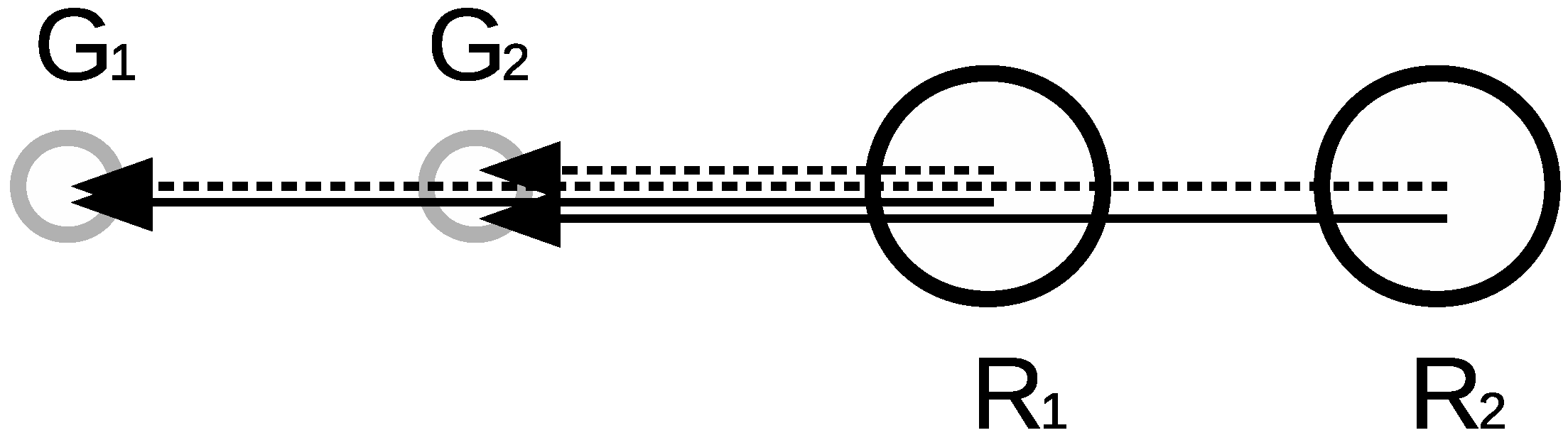
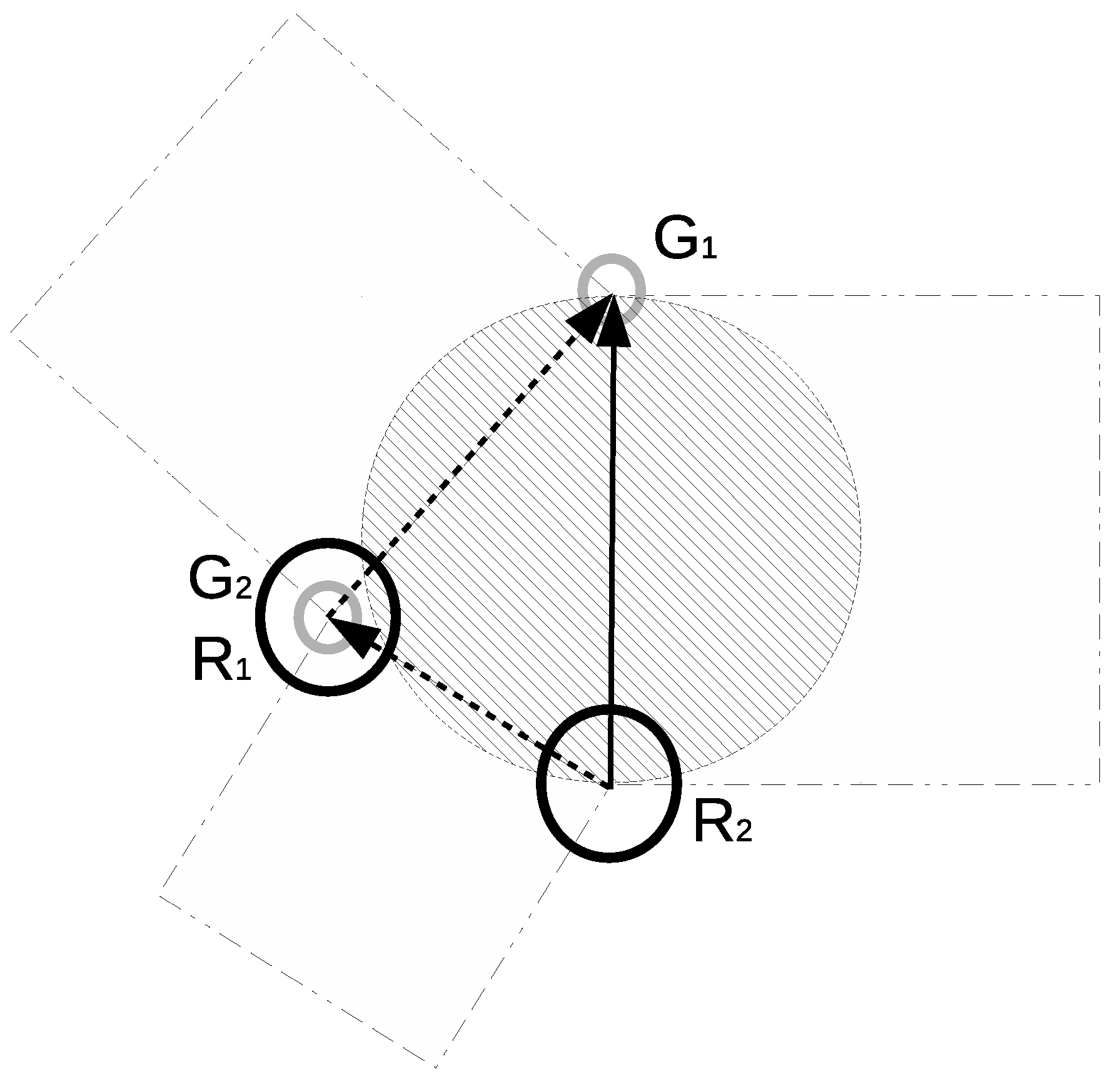
Figure 8 shows a case in which two robots and their goals lie on a straight line. Initially goal 2 is assigned to robot 1 and goal 1 is assigned to robot 2. This situation caused a saddle point because during the motion to the goal stays on the path of . One can observe that the shortest path criterion () produces exactly the same result for both possible goal assignments, while quadratic one () produces the result marked by continuous arrows. By the assignment and the goals can be reached by the robots without bypass manoeuvre. This is one of the examples showing the significant advantage of the quadratic criterion over the shortest path criterion proposed in [23].
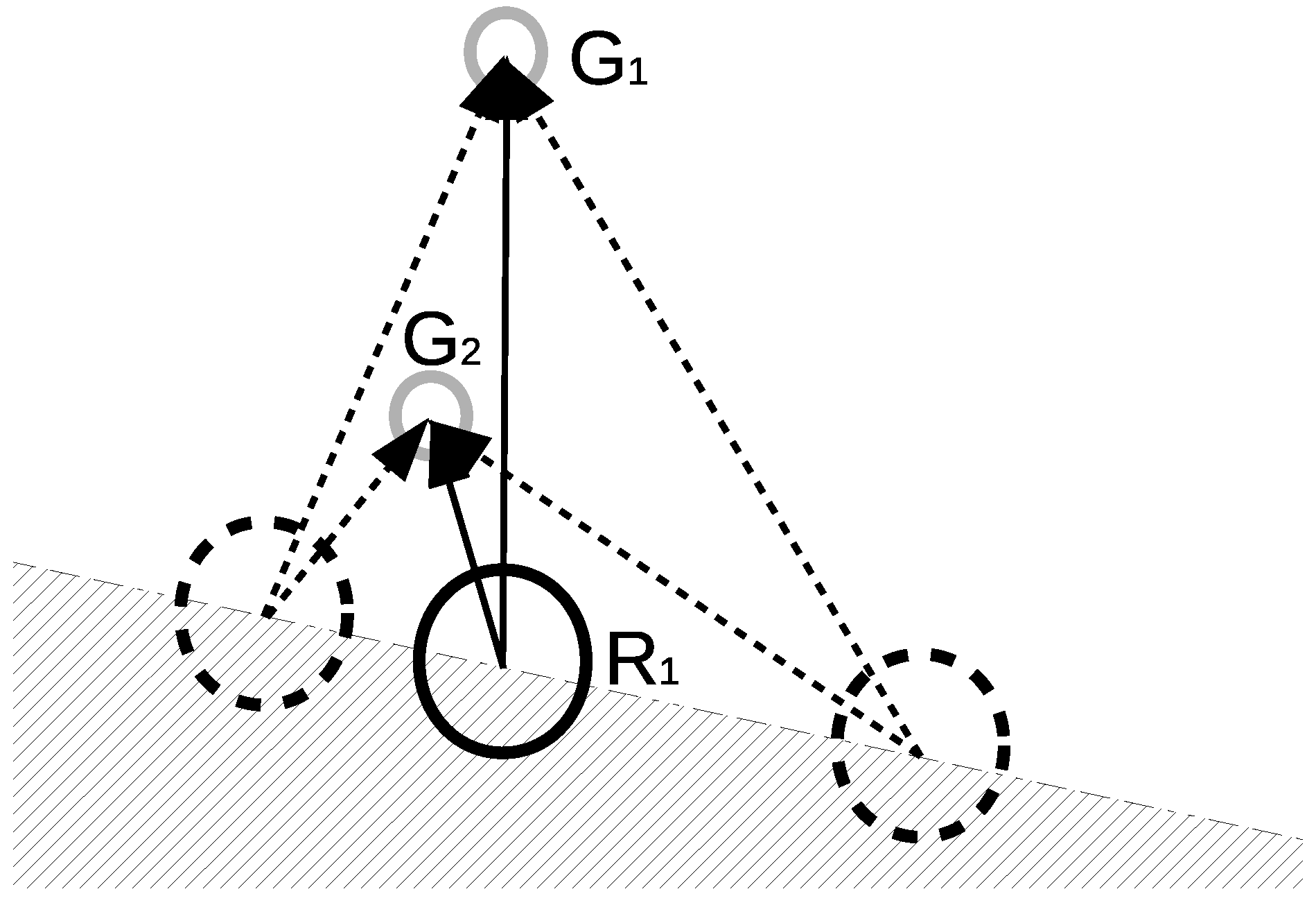
In Figure 9 is exactly at the goal assigned to it. was assigned to . The quadratic criterion resulted in the opposite assignment (continuous arrows). Notice that for the shortest path criterion the collision avoidance interaction between and was possible. For this type of situation the quadratic criterion resulted in goal exchange for all locations in the hatched circle. The opposite situation is presented in Figure 10. Fields of squares shown in the figures represent values of cost functions for two possible goal assignments (compare two left-hand side squares with right-hand square). The quadratic criterion resulted (in comparison to the shortest path) in a higher cost function for assigning far goals to the robots. It favoured a larger number of short assignments instead of the lower number of farther ones. This promoted the reduction of collision interaction situations.
In Figure 11 certain positions of the robot and goals and have been assumed. If robot is located in the hatched area the quadratic criterion assigns it to , otherwise it is assigned to . Some initial configuration may have led to temporary collision interaction states (i.e., when initially is located to the left of the ) but the saddle point occurrence was not possible. Dashed circles on the sides represent examples of boundary locations (for goal exchange) of the robot .
The considered cases do not cover all possible scenarios, but since there is no formal guarantee that the number of collision avoidance interactions between agents is reduced, they illustrate, together with simulation results, that in typical situations goal exchange procedure leads to the simplification of the control task.
9. Ensuring Integrity
As the goal exchange process involves two agents that are physically separated machines and they communicate through a wireless link the goal exchange process is at the risk of failure. Using a reliable communication protocol like Transmission Control Protocol (TCP) and dividing the process into a sequence of stages acknowledged by the remote host the fault-tolerance of the system can be increased. Assuming that the transmitted packets are encrypted (which is standard nowadays) and the implementation is relatively simple (the author believes that software bugs can be corrected) byzantine fault tolerance (BFT) [27] is not considered here.
The first stage of the goal exchange process is establishing the connection between agents. It is proposed to use the TCP connection because this protocol uses sequence numbers, acknowledgements, checksums and it is the most reliable, widely used communication protocol. Agents know network addresses of the other agents. They can be given in advance, provided by the higher-level system or obtained using a dedicated network broadcasting service. The attempt to connect to the agent that is already involved in the goal exchange process should be rejected. This can be easily and effectively implemented using TCP.
The second stage is transmission of the robot location coordinates and the goal from agent one to another. The receiver computes (Equation (32)) and sends back the obtained value. If agent closes the connection, otherwise they go to the third step.
The third step is a goal exchange that is the most critical part of the process. It must be guaranteed that no goal stays unassigned and no goal can be assigned to more than one robot in the case of agent/communication failure. To fulfil this condition the goal exchange must have all properties of database transaction: it must be atomic, consistent, isolated and durable. In practice this idealistic solution can be approximated by applying one of the widely used algorithms: two-phase commit protocol [28], three-phase commit protocol [29], or Paxos [30]. All of them introduce a coordinator block that is the central point of the algorithm. It can be run (for example as a separate process) on the one of the machines involved in the goal exchange procedure. Notice that in the case of failure (communication error, agent failure, etc.) the operation of goal exchange is aborted. This leads to slower convergence of robots to their desired values but is not critical for the task execution.
10. Simulation Results for Goal Exchange
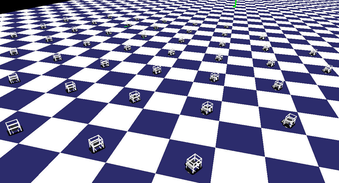
This section presents numerical simulation of the algorithm extended with goal exchange procedure. The initial conditions are exactly the same as in Section 4 (results for the algorithm without goal exchange). The parameters of the controllers were also the same. The initial value of the permutation matrix was the identity matrix .
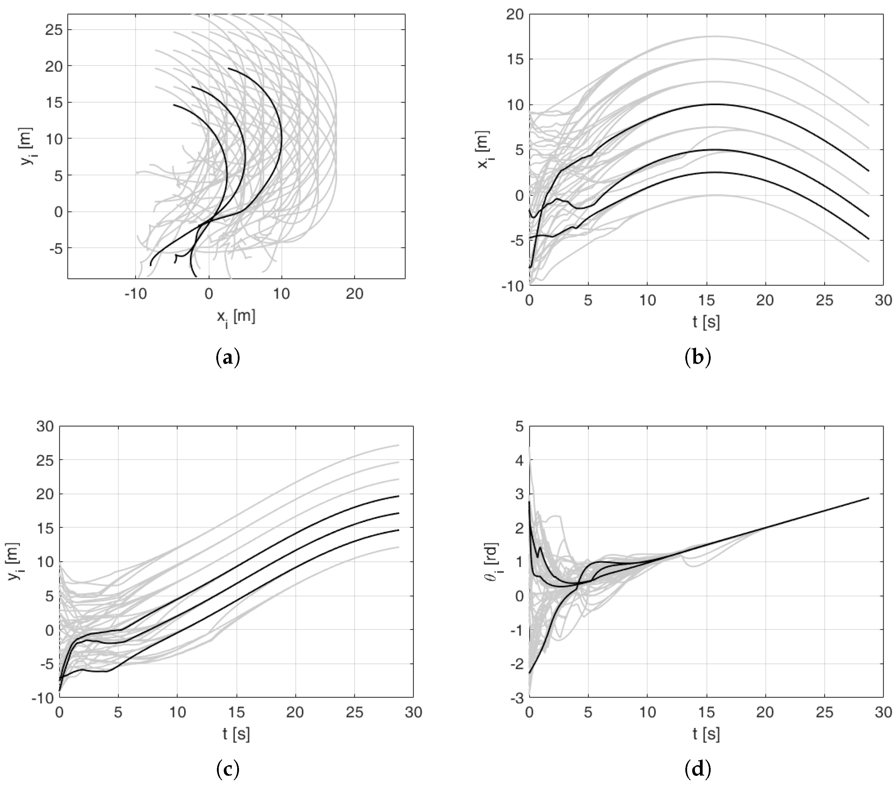
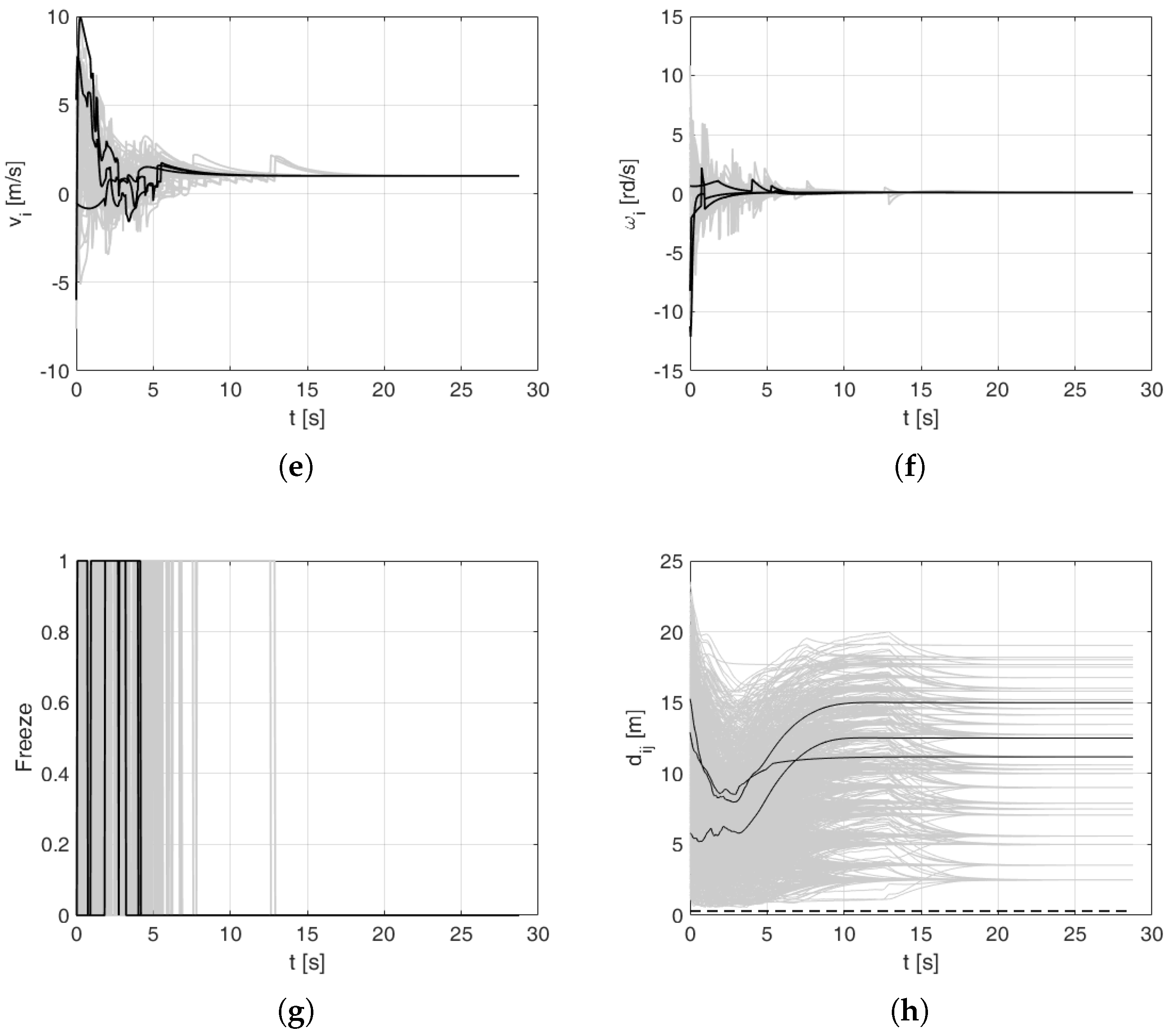
Figure 12a shows paths of robots on the plane. As in the previous experiment signals of 3 robots (out of 48) are highlighted in black. Figure 12b,c present graphs of x and y coordinates as a function of time. The robots converge to the desired values in less than 20 s, a significantly better result than 115 s (without goal exchange). This experiment was completed at 28 s due to faster convergence. Figure 12d shows a time graph of the orientations. In Figure 12e,f linear and angular controls are plotted. They reach constant values in less than 20 s. Figure 12g presents a time graph of the freeze procedure (refer to Assumption 2). It can be seen that the last collision avoidance interaction ends at 13 s. In Figure 12h relative distances between robots are shown. No pair of robots reaches inter-agent distance lower than or equal to 0.3 m (dashed line). It means that no collision has occurred.
Notice that in the presented simulation no communication delay of the goal exchange procedure was taken into account. Depending on the quality of the network single goal exchange may take even hundreds of milliseconds. On the other hand, as the procedure involves only a pair of agents, many of such pairs can execute goal exchange at the same time. Of course another limitation was the bandwidth of the communication network. These issues will be investigated by the author in the near future. In the presented numerical simulations the number of goal switchings was 238, which is a significant number.
Visualizations of the exemplary experiments are available on the website http://wojciech.kowalczyk.pracownik.put.poznan.pl/research/target-assignment/ts.html.
11. Simulation Results for Saturated Wheel Controls
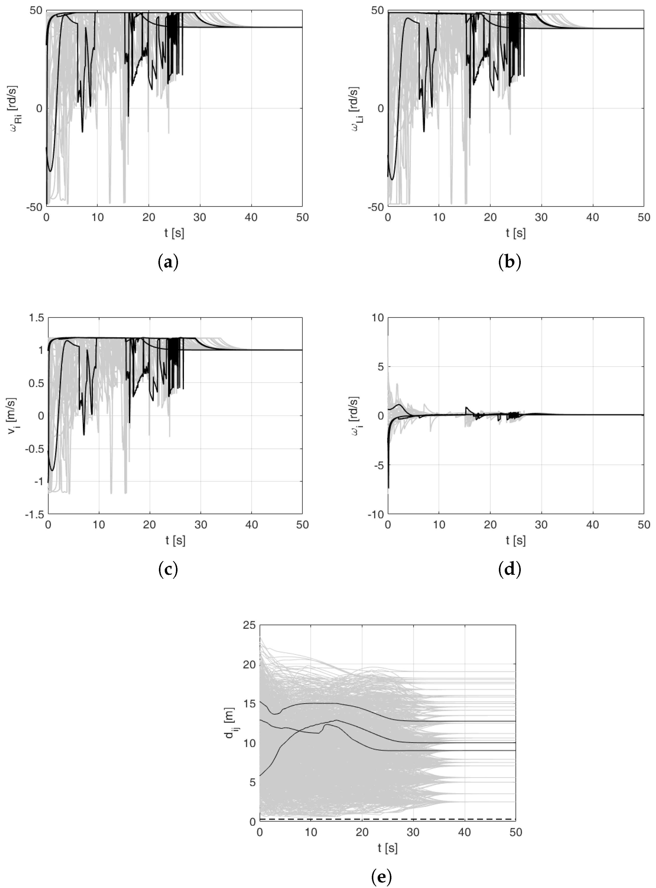
As the APFs used to avoid collisions are unbounded, the algorithm should be tested for the limited wheel velocities (resulting from the motor velocity limits). This section presents a numerical simulation for the mobile robots with the wheel diameter of 0.0245 m, the distance between wheels amounting to 0.148 m and the maximum angular velocity of 48.6 rd/s.
A special scaling procedure was applied to the wheel controls. The desired wheel velocities were scaled down when at least one of the wheels exceeds the assumed limitation. The scaled control signal is calculated as follows:
where
and
where , denote right and left wheel angular velocity, is the predefined maximum allowed angular velocity for each wheel.
Figure 13a,b show time graphs of the right and left wheels of the platforms. As in the previous experiments, signals of three robots (out of 48) are highlighted in black. It can be clearly observed that both of them were limited to ±48.6 rd/s. Linear and angular velocities of the platform are shown in Figure 13c,d. Their velocities are lower in comparison to the non-limited case (refer to Figure 12e,f). Figure 13e presents relative distances between the robots. The area below dashed line represents the collision region. It can be seen that no pair of robots has reached it—no collision occurred during this experiment.
12. Conclusions
This paper presents a new control algorithm for the formation of non-holonomic mobile robots. Inter-agent communication is used to check if exchange of goals between robots reduces the system’s overall Lyapunov-like function and the sum of position errors squared. The procedure is verified by numerical simulations for large group of non-holonomic mobile robots moving in the formation. The simulations also include the case in which wheel velocity controls are limited. A significant improvement of system convergence is shown. The author plans to conduct extensive tests of the presented algorithm on real two-wheeled mobile robots in the near future.
Funding
This work is supported by statutory grant 09/93/DSPB/0811.
Conflicts of Interest
The authors declare no conflict of interest.
References
- Khatib, O. Real-time Obstacle Avoidance for Manipulators and Mobile Robots. Int. J. Robot. Res. 1986, 5, 90–98. [Google Scholar] [CrossRef]
- Leitmann, G.; Skowronski, J. Avoidance Control. J. Optim. Theory Appl. 1977, 23, 581–591. [Google Scholar] [CrossRef]
- Leitmann, G. Guaranteed Avoidance Strategies. J. Optim. Theory Appl. 1980, 32, 569–576. [Google Scholar] [CrossRef]
- De Wit, C.C.; Khennouf, H.; Samson, C.; Sordalen, O.J. Nonlinear Control Design for Mobile Robots. Recent Trends Mob. Rob. 1994, 121–156. [Google Scholar] [CrossRef]
- Morin, P.; Samson, C. Practical stabilization of driftless systems on Lie groups: The transverse function approach. IEEE Trans. Autom. Control 2003, 48, 1496–1508. [Google Scholar] [CrossRef]
- Kowalczyk, W.; Michałek, M.; Kozłowski, K. Trajectory Tracking Control with Obstacle Avoidance Capability for Unicycle-like Mobile Robot. Bull. Pol. Acad. Sci. Tech. Sci. 2012, 60, 537–546. [Google Scholar] [CrossRef]
- Mastellone, S.; Stipanovic, D.; Spong, M. Formation control and collision avoidance for multi-agent non-holonomic systems: Theory and experiments. Int. J. Robot. Res. 2008, 107–126. [Google Scholar] [CrossRef]
- Do, K.D. Formation Tracking Control of Unicycle-Type Mobile Robots With Limited Sensing Ranges. IEEE Trans. Control Syst. Technol. 2008, 16, 527–538. [Google Scholar] [CrossRef]
- Kowalczyk, W.; Kozłowski, K.; Tar, J.K. Trajectory Tracking for Multiple Unicycles in the Environment with Obstacles. In Proceedings of the 19th International Workshop on Robotics in Alpe-Adria-Danube Region (RAAD 2010), Budapest, Hungary, 23–27 June 2010; pp. 451–456. [Google Scholar] [CrossRef]
- Kowalczyk, W.; Kozłowski, K. Leader-Follower Control and Collision Avoidance for the Formation of Differentially-Driven Mobile Robots. In Proceedings of the MMAR 2018—23rd International Conference on Methods and Models in Automation and Robotics, Międzyzdroje, Poland, 27–30 August 2018. [Google Scholar]
- Hatanaka, T.; Fujita, M.; Bullo, F. Vision-based cooperative estimation via multi-agent optimization. In Proceedings of the 49th IEEE Conference on Decision and Control (CDC), Atlanta, GA, USA, 15–17 December 2010; pp. 2492–2497. [Google Scholar] [CrossRef]
- Millan, P.; Orihuela, L.; Jurado, I.; Rubio, F. Formation Control of Autonomous Underwater Vehicles Subject to Communication Delays. IEEE Trans. Control Syst. Technol. 2014, 22, 770–777. [Google Scholar] [CrossRef]
- Yoshioka, C.; Namerikawa, T. Formation Control of Nonholonomic Multi-Vehicle Systems based on Virtual Structure. IFAC Proc. Vol. 2008, 41, 5149–5154. [Google Scholar] [CrossRef]
- Borrmann, U.; Wang, L.; Ames, A.D.; Egerstedt, M. Control Barrier Certificates for Safe Swarm Behavior. IFAC-PapersOnLine 2015, 48, 68–73. [Google Scholar] [CrossRef]
- Ames, A.D.; Xu, X.; Grizzle, J.W.; Tabuada, P. Control Barrier Function Based Quadratic Programs for Safety Critical Systems. IEEE Trans. Autom. Control 2017, 62, 3861–3876. [Google Scholar] [CrossRef]
- Srinivasan, M.; Coogan, S.; Egerstedt, M. Control of Multi-Agent Systems with Finite Time Control Barrier Certificates and Temporal Logic. In Proceedings of the 2018 IEEE Conference on Decision and Control (CDC), Miami Beach, FL, USA, 17–19 December 2018; pp. 1991–1996. [Google Scholar] [CrossRef]
- Akella, S. Assignment Algorithms for Variable Robot Formations. In Proceedings of the 12th International Workshop on the Algorithmic Foundations of Robotics, San Francisco, CA, USA, 18–20 December 2016. [Google Scholar]
- Caldeira, A.; Paiva, L.; Fontes, D.; Fontes, F. Optimal Reorganization of a Formation of Nonholonomic Agents Using Shortest Paths. In Proceedings of the 2018 13th APCA International Conference on Automatic Control and Soft Computing (CONTROLO), Ponta Delgada, Azores, Portugal, 4–6 June 2018. [Google Scholar]
- Alonso-Mora, J.; Baker, S.; Rus, D. Multi-robot formation control and object transport in dynamic environments via constrained optimization. Int. J. Robot. Res. 2017, 36, 1000–10217. [Google Scholar] [CrossRef]
- Alonso-Mora, J.; Breitenmoser, A.; Rufli, M.; Siegwart, R.; Beardsley, P. Image and Animation Display with Multiple Mobile Robots. Int. J. Robot. Res. 2012, 31, 753–773. [Google Scholar] [CrossRef]
- Desai, A.; Cappo, E.; Michael, N. Dynamically feasible and safe shape transitions for teams of aerial robots. In Proceedings of the 2016 IEEE/RSJ International Conference on Intelligent Robots and Systems (IROS), Daejeon Convention Center, Daejeon, Korea, 9–14 October 2016; pp. 5489–5494. [Google Scholar]
- Turpin, M.; Michael, N.; Kumar, V. Capt: Concurrent Assignment and Planning of Trajectories for Multiple Robots. Int. J. Robot. Res. 2014, 33, 98–112. [Google Scholar] [CrossRef]
- Panagou, D.; Turpin, M.; Kumar, V. Decentralized goal assignment and trajectory generation in multi-robot networks: A multiple Lyapunov functions approach. In Proceedings of the 2014 IEEE International Conference on Robotics and Automation (ICRA), Hong Kong, China, 31 May–5 June 2014; pp. 6757–6762. [Google Scholar] [CrossRef]
- Loria, A.; Dasdemir, J.; Alvarez Jarquin, N. Leader—Follower Formation and Tracking Control of Mobile Robots Along Straight Paths. IEEE Trans. Control Syst. Technol. 2016, 24, 727–732. [Google Scholar] [CrossRef]
- Michałek, M.; Kozłowski, K. Vector-Field-Orientation Feedback Control Method for a Differentially Driven Vehicle. IEEE Trans. Control Syst. Technol. 2010, 18, 45–65. [Google Scholar] [CrossRef]
- Khalil, H.K. Nonlinear Systems, 3rd ed.; Prentice-Hall: New York, NY, USA, 2002. [Google Scholar]
- Castro, M.; Liskov, B. Practical Byzantine Fault Tolerance. In Proceedings of the Third Symposium on Operating Systems Design and Implementation, New Orleans, LA, USA, 22–25 February 1999. [Google Scholar]
- Bernstein, P.; Hadzilacos, V.; Goodman, N. Concurrency Control and Recovery in Database Systems; Addison Wesley Publishing Company: Boston, MA, USA, 1987; ISBN 0-201-10715-5. [Google Scholar]
- Skeen, D.; Stonebraker, M. A Formal Model of Crash Recovery in a Distributed System. IEEE Trans. Softw. Eng. 1983, 9, 219–228. [Google Scholar] [CrossRef]
- Lamport, L. The Part-Time Parliament. ACM Trans. Comput. Syst. 1998, 16, 133–169. [Google Scholar] [CrossRef]
Figure 1.
Artificial potential functions (APF) as a function of distance to the centre of the robot (indexes omitted for simplicity).
Figure 1.
Artificial potential functions (APF) as a function of distance to the centre of the robot (indexes omitted for simplicity).

Figure 2.
Robot in the environment with an obstacle.

Figure 3.
Control system.

Figure 4.
Diagram of the control system in the collision avoidance mode.

Figure 5.
Numerical simulation 1: trajectory tracking for robots. (a) locations of robots in -plane, (b) x coordinates as a function of time, (c) y coordinates as a function of time, (d) robot orientations as a function of time, (e) linear velocity controls, (f) angular velocity controls, (g) ‘freeze’ signals, (h) distances between robots.

Figure 6.
Control system with goal switching.

Figure 7.
Two robot-goal assignment—case 1.

Figure 8.
Two robot-goal assignment—case 2.

Figure 9.
Two robot-goal assignment—case 3.

Figure 10.
Two robot-goal assignment—case 4.

Figure 11.
Two robot-goal assignment—case 5.

Figure 12.
Numerical simulation 2: trajectory tracking for robots with goal exchange. (a) locations of robots in -plane, (b) x coordinates as a function of time, (c) y coordinates as a function of time, (d) robot orientations as a function of time, (e) linear velocity controls, (f) angular velocity controls, (g) ‘freeze’ signals, (h) distances between robots.


Figure 13.
Numerical simulation 3: trajectory tracking for robots with goal exchange and saturated wheel controls. (a) right wheel velocities, (b) left wheel velocities, (c) linear velocity controls, (d) angular velocity controls, (e) distances between robots.
Figure 13.
Numerical simulation 3: trajectory tracking for robots with goal exchange and saturated wheel controls. (a) right wheel velocities, (b) left wheel velocities, (c) linear velocity controls, (d) angular velocity controls, (e) distances between robots.

© 2019 by the author. Licensee MDPI, Basel, Switzerland. This article is an open access article distributed under the terms and conditions of the Creative Commons Attribution (CC BY) license (http://creativecommons.org/licenses/by/4.0/).
Share and Cite
MDPI and ACS Style
Kowalczyk, W. Formation Control and Distributed Goal Assignment for Multi-Agent Non-Holonomic Systems. Appl. Sci. 2019, 9, 1311. https://0-doi-org.brum.beds.ac.uk/10.3390/app9071311
AMA Style
Kowalczyk W. Formation Control and Distributed Goal Assignment for Multi-Agent Non-Holonomic Systems. Applied Sciences. 2019; 9(7):1311. https://0-doi-org.brum.beds.ac.uk/10.3390/app9071311
Chicago/Turabian StyleKowalczyk, Wojciech. 2019. "Formation Control and Distributed Goal Assignment for Multi-Agent Non-Holonomic Systems" Applied Sciences 9, no. 7: 1311. https://0-doi-org.brum.beds.ac.uk/10.3390/app9071311
Note that from the first issue of 2016, this journal uses article numbers instead of page numbers. See further details here.