Integrating a Path Planner and an Adaptive Motion Controller for Navigation in Dynamic Environments


College of Systems Engineering, National University of Defense Technology, Changsha 410073, China
*
Author to whom correspondence should be addressed.
Appl. Sci. 2019, 9(7), 1384; https://0-doi-org.brum.beds.ac.uk/10.3390/app9071384
Submission received: 8 March 2019
/
Revised: 27 March 2019
/
Accepted: 29 March 2019
/
Published: 2 April 2019
(This article belongs to the Special Issue Mobile Robots Navigation)
Abstract
:Since an individual approach can hardly navigate robots through complex environments, we present a novel two-level hierarchical framework called JPS-IA3C (Jump Point Search improved Asynchronous Advantage Actor-Critic) in this paper for robot navigation in dynamic environments through continuous controlling signals. Its global planner JPS+ (P) is a variant of JPS (Jump Point Search), which efficiently computes an abstract path of neighboring jump points. These nodes, which are seen as subgoals, completely rid Deep Reinforcement Learning (DRL)-based controllers of notorious local minima. To satisfy the kinetic constraints and be adaptive to changing environments, we propose an improved A3C (IA3C) algorithm to learn the control policies of the robots’ local motion. Moreover, the combination of modified curriculum learning and reward shaping helps IA3C build a novel reward function framework to avoid learning inefficiency because of sparse reward. We additionally strengthen the robots’ temporal reasoning of the environments by a memory-based network. These improvements make the IA3C controller converge faster and become more adaptive to incomplete, noisy information caused by partial observability. Simulated experiments show that compared with existing methods, this JPS-IA3C hierarchy successfully outputs continuous commands to accomplish large-range navigation tasks at shorter paths and less time through reasonable subgoal selection and rational motions.
1. Introduction
Navigation in dynamic environments plays an important role in computer games and robotics [1], such as generating realistic behaviors of Non-Player Characters (NPCs) and meeting practical applications of mobile robots in the real world. In this paper, we focus on the navigation problems of nonholonomic mobile robots [2] with continuous control in dynamic environments, as this is an important capability for widely used mobile robots.
Conventionally, sampling-based and velocity-based methods are used to support the navigation of mobile robots [1]. Sampling-based methods, such as Rapidly Exploring Trees (RRTs) [3] and Probabilistic Roadmap (PRM) [4], deal with environmental changes by reconstructing pre-built abstract representations at high time costs. Velocity-based methods [5] compute avoidance maneuvers by searching over a tree of avoidance maneuvers, which require high time consumption in complex environments.
Alternatively, many researchers focus on learning-based methods—mainly those including Deep Learning (DL) and Deep Reinforcement Learning (DRL). Although DL achieves great performance in robotics [6], it is hard to apply DL in this navigation problem, since collecting considerable amounts of labeled data requires much time and energy for researchers. By contrast, DRL does not need supervised samples, and has been widely used in video games [7] and robot manipulation [8]. There are two categories of DRL (i.e., value-based DRL and policy-based DRL). Compared with valued-based DRL methods, policy-based methods are more suitable for us to handle continuous action spaces. Asynchronous Advantage Actor-Critic (A3C), which is a policy-based method, is widely used in video games and robotics [9,10,11], since it can greatly decrease training time and meanwhile increase performance [12]. However, several challenges need to be tackled if A3C is used to deal with robot navigation in dynamic environments.
First, robots trained by A3C are vulnerable to local minima such as box canyons and long barriers, which most DRL algorithms cannot effectively resolve. Second, rewards are sparsely distributed in the environment, for there may be only one goal location [9]. Third, robots with limited visibility can only gather incomplete and noisy information from current environmental states due to partial observability [13], and in this paper, we are concerned with robots that just know the relative positions of obstacles within a small range.
Given that an individual DRL approach can hardly drive robots out of regions of local minima and navigate them in changing surroundings, this paper proposes a hierarchical navigation algorithm based on a two-level architecture, whose high-level path planner efficiently searches for a sequence of subgoals placing at the exits of those regions, while the low-level motion controller learns how to tackle moving obstacles in local environments. Since JPS+ (P), which is a variant of JPS+, on average answers a path query faster by up to two orders of magnitude over traditional A* [14], the path planner uses it to find subgoals between which the circumstances are relatively simple and easy for A3C to train and converge to a motion policy.
To tackle two other challenges regarding learning, we propose an improved A3C (IA3C) for the motion controller by making some improvements to A3C. IA3C combines a modified curriculum learning with reward shaping to build a novel reward function framework in order to solve the problem of sparse rewards. In the framework, the modified curriculum learning adds prior experiences to set different difficulty levels of navigation tasks and adjusts the frequencies of different tasks by considering features of navigation. Reward shaping plays an auxiliary role in each task to speed up training efficiency. Moreover, IA3C builds a network architecture based on long short-term memory (LSTM), which integrates current observation and hidden state from historical observations to estimate current state. Briefly, the proposed method integrates JPS+ (P) and IA3C, named JPS-IA3C; this model can realize long-range navigation in complex and dynamic environments by addressing mentioned challenges.
2. Related Work
This section will introduce related works regarding sampling-based and velocity-based methods, DL and DRL. Sampling-based and velocity-based methods are classical navigation methods that are not suitable for dealing with environmental changes. Learning-based methods such as DL and DRL can improve the learning ability of mobile robots to quickly adapt to new environments. DL requires considerable amounts of labeled data, which is difficult to be collected, while DRL does not need prior knowledge.
2.1. Sampling-Based and Velocity-Based Methods
Autonomous navigation in dynamic environments is challenging, since the planner is forced to frequently adjust its planned results for handling dynamic objects such as moving obstacles. Velocity obstacle (VO) [5] can simply consider dynamic constraints to compute trajectories of robots via the concept of velocity obstacles that denote the robot’s velocities causing a collision with obstacles soon. However, computing maneuvers by velocity obstacles has low efficiency for real-time applications. Sampling-based methods such as PRM and RRT are popular in robotics, benefitting from advantages regarding efficiency and robustness [15]. This kind of method can solve high-dimensional planning problems by approximating C-space. Nevertheless, in dynamic environments, PRM needs to recheck edge connection [16], and RRT is required to modify the pre-built exploring tree [15], which further decrease time efficiency when environments become more dynamic. Consequently, the above-mentioned model-based methods still suffer from essential disadvantages that cannot realize time-saving navigation in dynamic environments, so as to hinder the robot’s navigation capabilities.
2.2. Deep Learning
In recent years, as deep neural networks show great potential for solving complex estimation problems, a rapidly growing trend of utilizing DL techniques has appeared in robotics tasks. For navigation based on visual information, Chen et al. [17] used deep neural networks to learn how to recognize objects from the image, and then determined discrete actions such as turning left and turning right according to the identified information. Gao et al. [18] proposed a novel deep neural network architecture, Intention-Net, to track the planned path by mapping monocular images to four discrete actions such as going forward. Since the action is discrete, the navigation behaviors in above-mentioned researches are rough and likely to be unfeasible. For navigation based on range information, Pfeiffer et al. [19] used demonstrative data to train a DL model that can control the robot through inputting the data from laser sensors and the target position. However, since a large number of labeled data are required for training the above DL models, it may be unpractical for real-world applications.
2.3. Deep Reinforcement Learning
Autonomous navigation demands two essential building blocks: perception and control. Similar to the above-mentioned studies about DL, many research studies [20] about applying DL in navigation are pure perception, which means that agents passively receive observations and infer desired information. Compared with pure perception, control goes one step further, seeking to actively interact with the environment by executing actions [21]. Then, navigation becomes a problem of sequential decisions. DRL is very suitable for solving it, which is proved by reference [7] in game and reference [8] in robotics. Since DRL methods can deal with better full observable states than partial states, lots of studies [9,10,22] about applying DRL in navigation focus on static environments. Regarding dynamic environments, Chen et al. [23] proposed a time-efficient approach based on DRL for socially aware navigation. However, to calculate the reward based on social norms, the motion information of pedestrians are known in advance, which are not reliable in real-world applications, since it is not precise to estimate information by sensor readings.
Given that it is difficult for an individual DRL method to solve the navigation problem, hierarchical approaches are widely researched in the literature [24,25,26]. Lei et al. [26] combined A* and least-squares policy iteration for mobile robot navigation in complex environments. Aleksandra et al. [25] integrated sampling-based path planning with reinforcement learning (RL) agents for indoor navigation and aerial cargo delivery. The aforementioned methods can only handle navigation in static environments. Kato et al. [24] combined value-based DRL with A* on topological maps to solve navigation in environments with pedestrians. However, the experiment results are not well applied in dynamic environments, since the learned policy is reactive and the way of taking observations as states is inaccurate, which may lead to irrational behaviors and even collisions with obstacles.
Compared with the above hierarchical methods, our hierarchical navigation algorithm can generate better waypoints by JPS+ (P) and navigate in dynamic environments via IA3C.
3. The Methodology
In this section, we at first briefly introduce the problem and model the virtual tracked robot. Next, we present the architecture of the proposed navigation method. Finally, we describe the global path planner based on JPS+ (P) and the local motion controller based on IA3C in detail.
3.1. Problem Description
In this paper, the problem of navigation can be stated as follows: on an initially known map, the mobile tracked robot that is only equipped with local laser sensors autonomously navigate without colliding with moving obstacles via continuous control. Since environments with moving obstacles are dynamic and uncertain, this navigation task is difficult to be dealt with, and is an non-deterministic polynomial-hard problem [27].
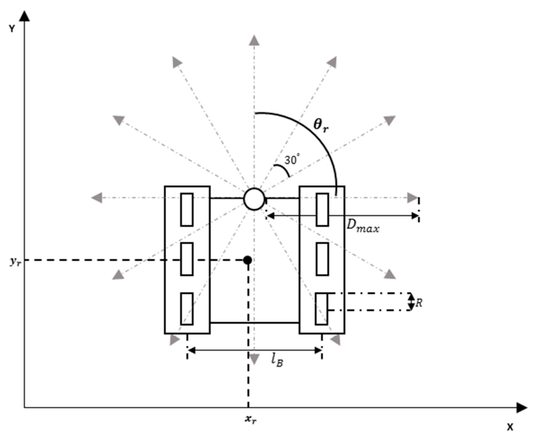
In this paper, we adopt the Cartesian coordinate system. The structure of the tracked robot is shown in Figure 1. The position state of the tracked robot is defined as by the global coordinate of the map, where and are the tracked robot’s horizontal and vertical coordinates, respectively, and is the angle between the forward orientation of the tracked robot and the abscissa axis. Twelve laser sensors equipped at the front of the tracked robot can sense the nearby surroundings 360 degrees. The detection angle of each laser sensor is 30 degrees. The max detection distance is . The robot is controlled by the left and right tracks. The kinematic equations were as follows:
where R is the radius of the driving wheels in the tracks; and denote the angular velocity (rad) of left tracks and right tracks; and respectively denote the angular acceleration of left tracks and right tracks (rad), and denotes the distance between the left and right tracks.
3.2. The Architecture of the Proposed Algorithm
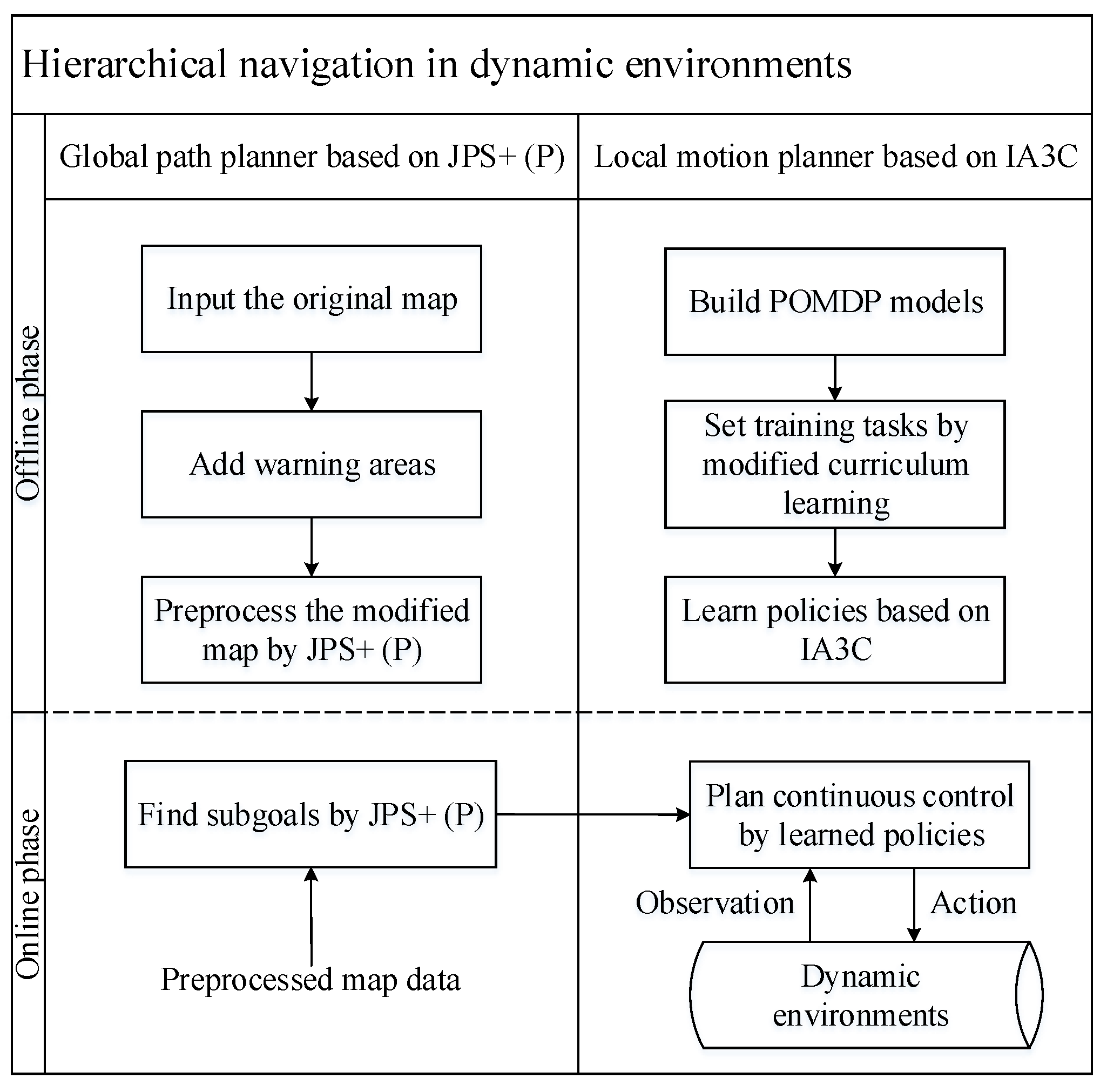
As mentioned above, JPS-IA3C resolves the robot navigation in a two-level manner: the first for the efficient global path planner, and the second for the robust local motion controller. Figure 2 shows the architecture of the proposed algorithm.
As shown in Figure 2, at the offline phase of the path planner whose goal is to efficiently find subgoals, we first define a warning circled area for every obstacle by taking the self-defined safety distance and sizes of robots into consideration. It is perilous for robots to touch these areas, since they are close to obstacles. Then, based on the modified map, JPS+ (P) calculates and stores the topology information of a map by preprocessing. In the online phase, JPS+ (P) uses canonical ordering known as diagonal-first to efficiently find subgoals based on preprocessed map data.
At the offline step of the motion controller whose task is planning feasible paths between adjacent subgoals, we firstly extract key information about robots and environments to build a partially observable Markov decision process (POMDP) model, which is a kind of formal description about partially observable environments for IA3C. Then, we quantify the difficulty of navigation and set training plans via a modified curriculum learning. Next, IA3C is used to learn navigation policies with high training efficiencies. At the online step, which is guided by subgoals, the robot receives sensor data about local environmental observations and then plans continuous control by learned policies. Next, the robot executes actions in dynamic environments and simultaneously updates its trajectories by kinematic equations. The online phase of the local motion planner denotes the interaction between robots and environments. Note that IA3C works on the original map, because warning areas cannot be detected by sensors.
There are two advantages of our method for robot navigation. The first advantage is that its high-level path planner can plans subgoals by preprocessing data and canonical ordering averagely within dozens of microseconds, so as to quickly respond to online tasks and avoid the so-called first-move lags [28]. Besides, it decomposes a task of long-range navigation into a number of local controlling phases between every two consecutive subgoals. Actually, traversing each of these segments, where there are no twisty terrains, rids our RL-driven controller of local minima. Therefore, benefitting from the path planner, the proposed algorithm can adapt to large-scale and complex environments.
The second advantage is that IA3C can learn near-optimal policies to navigate agents through adjacent subgoals in dynamic environments with kinematic and task constraints satisfied. There are two strengths of IA3C regarding learning to navigate. (1) To estimate complete environmental states, IA3C takes the time dimension into consideration by constructing an LSTM-based network architecture that can memorize information at different timescales. (2) Curriculum learning is useful for agents to gradually master complex skills, but conventional curriculum learning has been proven to be ineffective at training LSTM layers [29]. Therefore, we improve curriculum learning by adjusting distributions of different difficult samples over time and combine it with reward shaping [30] to build a novel reward function framework that can address the challenge of spare rewards. Moreover, due to the generalization of the local motion controller, the proposed algorithm can navigate robots to unseen environments without retraining.
3.3. Global Path Planner Based on JPS+ (P)
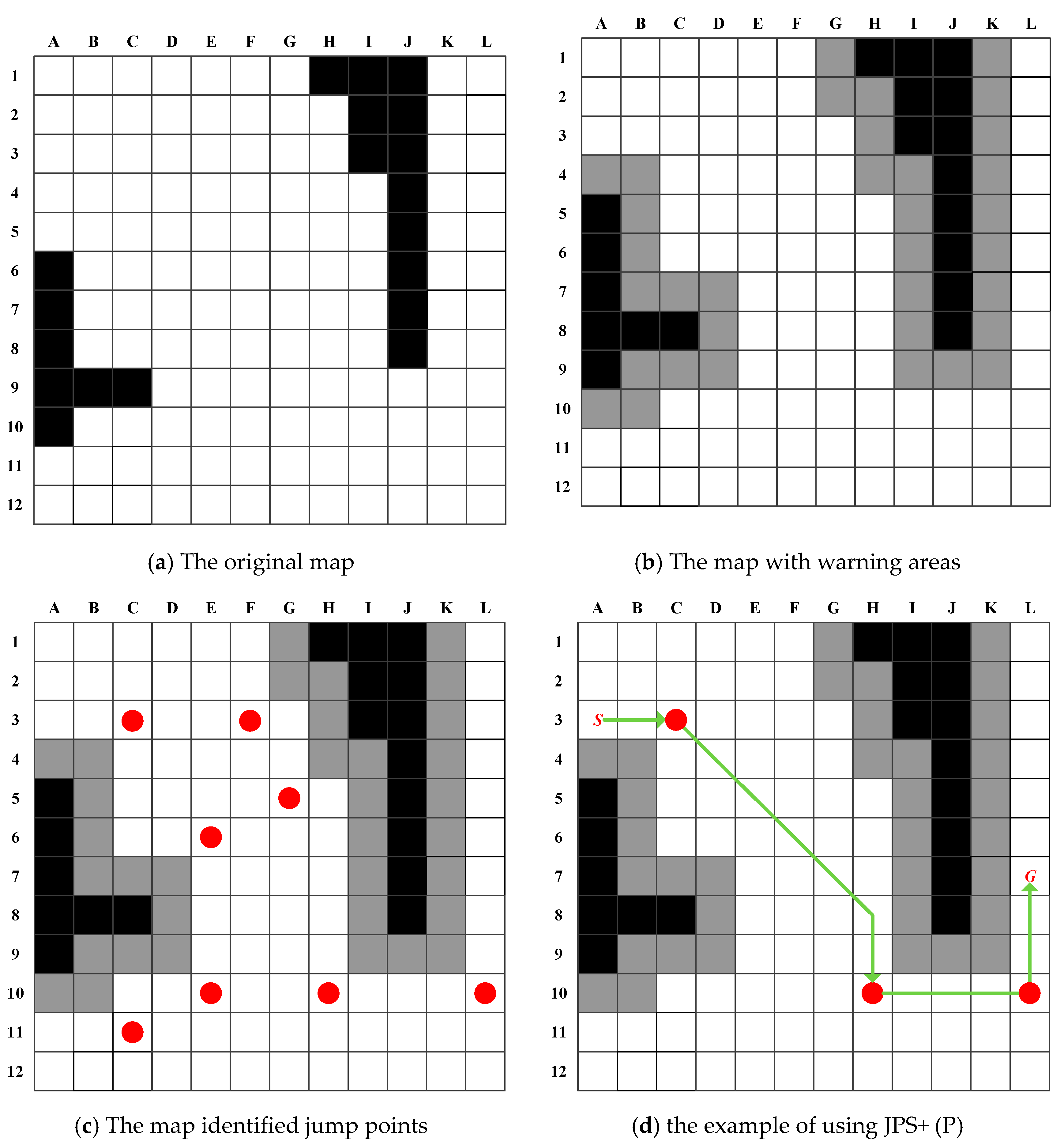
Figure 3a–c shows the offline work of the path planner, which includes constructing warning areas and identifying subgoals by preprocessing. Without the warning areas computed based on distance maps, the subgoals would be too close to the obstacles for moving robots, which increase the probabilities of colliding with walls.
During the process of constructing warning areas, the dynamic brushfire algorithm [31] is used to build the Euclidean distance map (EDM) based on the original map. The minimum distance between robots and obstacles is limited by the physical radius of robots; thus, a user-defined safety distance is required to increase insurance for robots that carry out important tasks. Therefore, the size of warning areas is determined by the above two factors (Figure 3b).
In the JPS family, jump points are the intermediate points that are necessary to travel through for at least one optimal path [14]. To put it simply, JPS and JPS+ call locations where a cardinal search can branch itself to wider areas due to obstacle disappearance in the incoming direction straight jump points. For example, in Figure 3c, an eastern search from A3 wraps around obstacles at C3, and then broadens itself to the southeastern areas. Besides straight nodes, they identify diagonal jump points linking two straight ones where the incoming diagonal search from the first can turn cardinally to reach the second. JPS+ improves JPS through exploiting diagonal-first ordering in the offline phase, and storing for each traversable cell the distance to the nearest jump point or obstacle that can be reached in every cardinal or diagonal direction. More details can be found in [14,32].
This paper applies JPS+ (P), which is an enhanced version of JPS+ with an intermediate pruning trick; thereby, the optimal path in Figure 3d will not generate and expand the diagonal jump point H8. JPS+ (P) requires the same preprocessing overheads to JPS+, but has stronger online efficiency.
To sum up, JPS+ (P)—which we borrow from [32]—has obvious advantages over other high-level planners of hierarchical methods in the literature [24,25,26], in terms of its low precomputation costs and outstanding online performance. Moreover, it serves as an ideal for the location distribution of jump points, providing a DRL-based controller with meaningful subgoals that can completely throw the problem of local minima out of consideration.
3.4. Local Motion Controller Based on IA3C
3.4.1. Construction of Navigation POMDP
In [26], the problem of local navigation is decomposed into two subproblems (i.e., approaching targets and avoiding obstacles), which easily leads to local optimal policies due to simplifying the problem by adding prior experiences. In JPS-IA3C, to acquire optimal navigation policies, the motion controller directly builds models for the entire navigation problem.
According to [24], current observations are regarded as states, whose representation is non-Markovian in the proposed navigation problem, since current observations including sensor readings do not contain all of the states of dynamic environments, such as the velocities of obstacles. To tackle the above problems, a POMDP is built to describe the process of navigating robots toward targets without colliding obstacles. It can capture dynamics in environments by explicitly acknowledging that sensations received by agents are only partial glimpses of the underlying system state [13].
A POMDP is formally defined as a tuple of , where , and , are the state, action, and observation spaces, respectively. The state-transition function, , denotes the probability of transferring the current state to next state by executing action . The reward function, , denotes the immediate reward obtained by agents, when the current state is transferred to the next state by taking action . The observation function denotes the probability of receiving observation after taking action in state [33].
In dynamic and partially observable environments, the robot cannot directly obtain exact environmental states. However, it can construct its own state representation about environments, which are called belief states . There are three ways of constructing belief states, including the complete history, beliefs of the environment state, and recurrent neural networks. Owing to the powerful nonlinear function approximator, we adopt a typical recurrent neural network: LSTM. The equation of constructing via LSTM is described as follows:
where denotes the activation function, and denote the weight parameters of neural networks, and denotes the observation at time .
The definitions of this POMDP are described in Table 1.
In this POMDP, observation () denotes the reading of sensor . The range of is [0, 5]. Observation denotes the normalization value of the distance between the robot and the target. The absolute value of observation denotes the angle between the direction of the robot toward the goal and the robot’s orientation. The range of is . When the goal is on the left side of the robot’s direction, the value of is positive; otherwise, it is negative. To support the navigation ability of our approach, the observation space of the robot is expanded to include the last angular accelerations and angular velocities. Observations are described in Section 3.1. The ranges of are both .
The action space is continuous, including the angular accelerations of the left and right tracks, so that the robot has great potential to perform flexible and complex actions. Besides, taking continuous angular accelerations as actions, trajectories updated by kinematic equations can preserve G2 continuity [34].
In the reward function, denotes the goal tolerance. . denotes the brake distance for the robot. When the distance between the robot and the subgoal is less than , the robot gets a +10 scalar reward. When the robot collides with obstacles, it gets a −5 scalar reward. Otherwise, the reward is 0. However, the reward function is not suitable for this POMDP, since fewer samples with positive rewards are collected during the initial learning phase, which incurs difficult training and even non-convergence in complex environments. Some improvements in reward functions will be discussed in Section 3.4.3.
3.4.2. A3C Method
In DRL, there are some key definitions [30]. The value function denotes the expected return for the agent in a given state . The policy function denotes the probability of an action executed by the agent in a given state .
Compared with valued-based DRL methods such as Deep Q Network (DQN) and its variations, A3C as a representative policy-based method can deal with continuous state and action spaces, and be more time-efficient. A3C is an on-policy and online algorithm that can use samples generated by current policies to efficiently update network parameters and increase robustness [12].
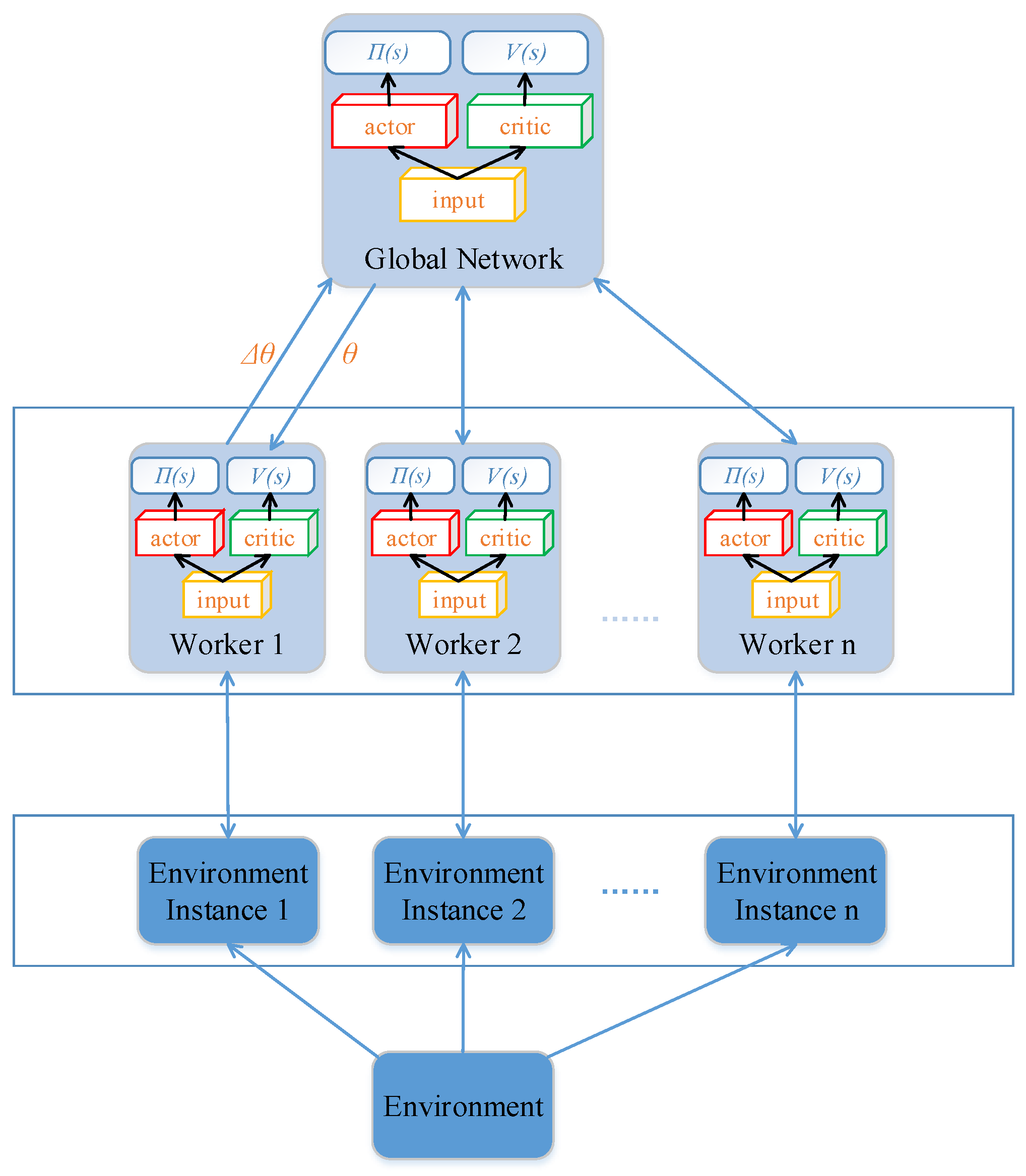
As shown in Figure 4, A3C asynchronously parallel executes multiple agents on multiple instances of the environment. All of the agents have the same local network architecture as the global network that is used to approximate policy functions and value functions. After the agent collects certain samples to calculate the gradient of its network, it uploads this gradient to the global network. Then, the agent downloads the global network to substitute its current network, after the global network updates its parameters by the uploaded gradient. Note that agents cannot upload their gradient simultaneously.
It is difficult for the predecessor of A3C, Actor-Critic (AC), to converge, since consecutive sequences of samples used to update networks have strong temporal relationships. To solve this problem, A3C adopts an asynchronous framework to construct independent and identically distributed training data. Compared with Deep Deterministic Policy Gradient (DDPG) [8], which uses experience replay to reduce the correlation between training samples, A3C can better decorrelate the agents’ data by using asynchronous actor-learners interacting with environments in parallel.
A3C includes two neural networks, actor-network and critic-network. Actor-network is used to approximate the policy function (i.e., ); it outputs the expectation and variance of the action distribution in continuous action spaces, and then samples an action from the built distribution. Critic-network used to approximate the value function (i.e., ); it outputs the estimation of the value function of the current state to optimize probabilities of choosing actions. As seen in Algorithm 1 [12], each actor-learner can share experiences through communicating with the global network, which can greatly increase the training efficiency. The condition of updating is every step or reaching the end of episode. The gradient of the actor-network is:
where is the entropy of the policy , and the hyper-parameter controls the strength of the entropy regularization term. is an estimate of the advantage function given by:
where can vary from state to state, and is upper-bounded by [12].
| Algorithm 1. Pseudo-code of each actor-learner in Asynchronous Advantage Actor-Critic (A3C). |
| 1: // : global shared parameters of actor-network and critic-network |
| 2: // : thread-specific parameters of actor-network and critic-network |
| 3: // : thread step counter |
| 4: // : max value for |
| 5: // : global shared counter |
| 6: // : max value for |
| 7: // : an instance of the environment |
| 8: |
| 9: Repeat |
| 10: |
| 11: |
| 12: |
| 13: = env.reset() |
| 14: While True |
| 15: = |
| 16: , = env.step() |
| 17: |
| 18: |
| 19: If terminal or |
| 20: upload the gradients of to |
| 21: update |
| 22: download the parameters of to |
| 23: If terminal |
| 24: break |
| 25: until () |
3.4.3. IA3C Method
Although A3C can be successfully applied in Atari Game and robot manipulation [12], it cannot be directly used in this navigation scenario due to the mentioned challenges. In Section 3.3, we discussed the challenge of local minima solved by the high-level path planner in JPS-IA3C. In this section, IA3C is proposed to address other two challenges, which are described as follows.
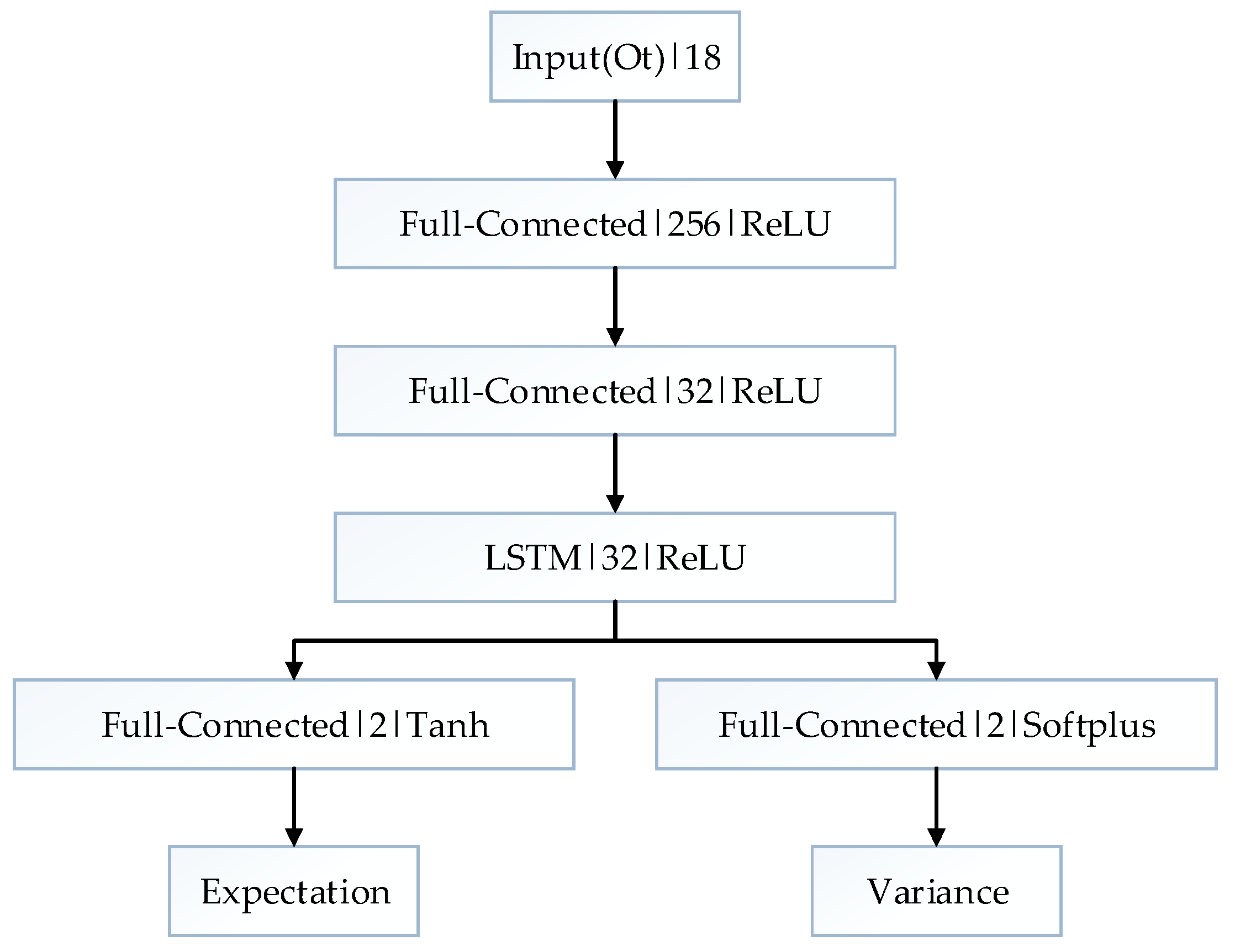
Firstly, an LSTM-based network structure can solve the problem of incomplete and noisy state information caused by partial observability. The original A3C is designed to solve MDPs that cannot precisely describe partially observable environments, but POMDPs can. In the proposed POMDP, the robot can only get range data about nearby environments by laser sensors, while velocities of obstacles as part of state information are unknown for the robot. The LSTM-based network architecture is constructed to solve the built POMDP, which takes current observation and abstract history information as input to estimate complete states. Since LSTM can store abstract information at different time scales, the proposed network can add the time dimension to infer hidden states. As shown in Figure 5, the observation is taken as the input of the network. The first hidden layer is a fully-connected (FC) layer with 215 nodes, and the second is an FC layer with 32 nodes. The last hidden layer is an LSTM layer with 32 nodes. The output layer outputs the expectation and variance of the Gaussian distributions of action spaces. Instead of directly outputting actions, the way of building distribution can introduce more randomness to increase the diversities of samples.
In the network architecture, FC layers can abstract key features from current observations. Then, an LSTM layer with recurrence mechanism takes current abstracted features and the last output of it as input, and then extracts high-level features based on complete state information. The last output layer is an FC layer that is used to determine the action distribution. In conclusion, the learning procedure of this network structure is first to abstract observation features, secondly to estimate complete state features, and finally to make decisions, which is similar to the process of memory and inference in human beings.
Secondly, to solve the problem of sparse reward, we make another improvement on A3C by building a novel reward function framework that integrates a modified curriculum learning and reward shaping. In the task of navigation, the robot only gets a positive reward when it reaches the goal, which means that positive rewards are sparsely distributed in large-scale environments. Curriculum learning can be used to speed up the process of training networks by gradually increasing the samples’ complexity in supervised learning [35]. In DRL, it can be used to tackle the challenge of sparse reward. Since original curriculum learning is not appropriate to train an LSTM-based network, we improve it by dividing whole learning tasks into two parts. The first part of learning tasks’ complexity is gradually increased, and the second part’s complexity is randomly chosen and not less than that of the first part. The navigation task is parameterized by distance (i.e., the initial distance between the goal and the robot) and the number of moving obstacles. Four kinds of learning tasks are designed through considering suitable difficult gradients, and each learning task has its own learning episodes (Table 2). Reward shaping is also a kind of useful way to reduce the side effects of the sparse reward problem. As shown in Table 3, the reward shaping means giving the robot early rewards before the end of the episode, but the early rewards must be much smaller than the reward received at the end of the episode [30].
Where denotes a hyper-parameter used to control the effect of early rewards, and denotes at time .
In summary, the above-mentioned reward function framework can increase the density of reward distribution in dynamic environments and improve the training efficiency to achieve better performance.
4. Experiments and Results
JPS-IA3C combines a geometrical path planner and a learning-based motion planner to navigate robots in dynamic environments. To verify the performances of the path planner, we evaluate JPS+ (P)’s ability to find subgoals on complex maps, and then compare it with the ability of A*. Then, to evaluate the effectiveness of the motion planner, we validate the capabilities of the LSTM-based network architecture and the novel reward function framework in the training process. Finally, the performance of JPS-IA3C will be evaluated in large-scale and dynamic environments. To acquire the map data of tested environments, we firstly constructed grayscale maps via real data from laser sensors, and then transform them to grid maps (if a cell is occupied by an obstacle, this cell is set to be untraversable; otherwise, it is traversable). The distance measurement accuracy can be improved by optimization methods [36]. The dynamics of environments are caused by moving obstacles that imitate the simple behaviors of people (i.e., linear motion with constant speed).
For simulation settings, we adopt numerical methods to compute the robot’s position via kinematic equations. Although smaller steps can achieve more precise results, they also lead to more computational consumptions and slower computation speed. To acquire high efficiencies, we select the step of simulation time as 0.1 .
The discounted factor is 0.99. The learning rates of the actor-network and critic-network are 0.00006 and 0.0004, respectively. The unrolling step is 7. The subgoal tolerance is 1.5, and the final goal tolerance is 1.0. Since subgoals roughly guide the robot, the subgoal tolerance is relatively large. In the training, we set the time interval of action choice to 2 , while the time interval decreases to 0.5 in the evaluation.
We run experiments on a 3.4-GHz Intel Core i7-6700 CPU with 16 GB of RAM.
4.1. Training Environment Settings
The training environment is a simple indoor environment whose size is 20 by 20 (Figure 6). A start point, a goal point, and the motion states of moving obstacles are randomly initialized in every episode so as to cover the entire state space as soon as possible. Moving obstacles denote people, robots, and other moving objects, which adopt the uniform rectilinear motion. The range of moving obstacles’ velocities is [0.08, 0.1]. The initial position is at the edge of the maximum detection distance of the robot, and the initial direction is roughly toward the robot. When the robot arrives at the goal or collides with obstacles, the current episode ends, and the next episode starts.
4.2. Evaluation of Global Path Planning
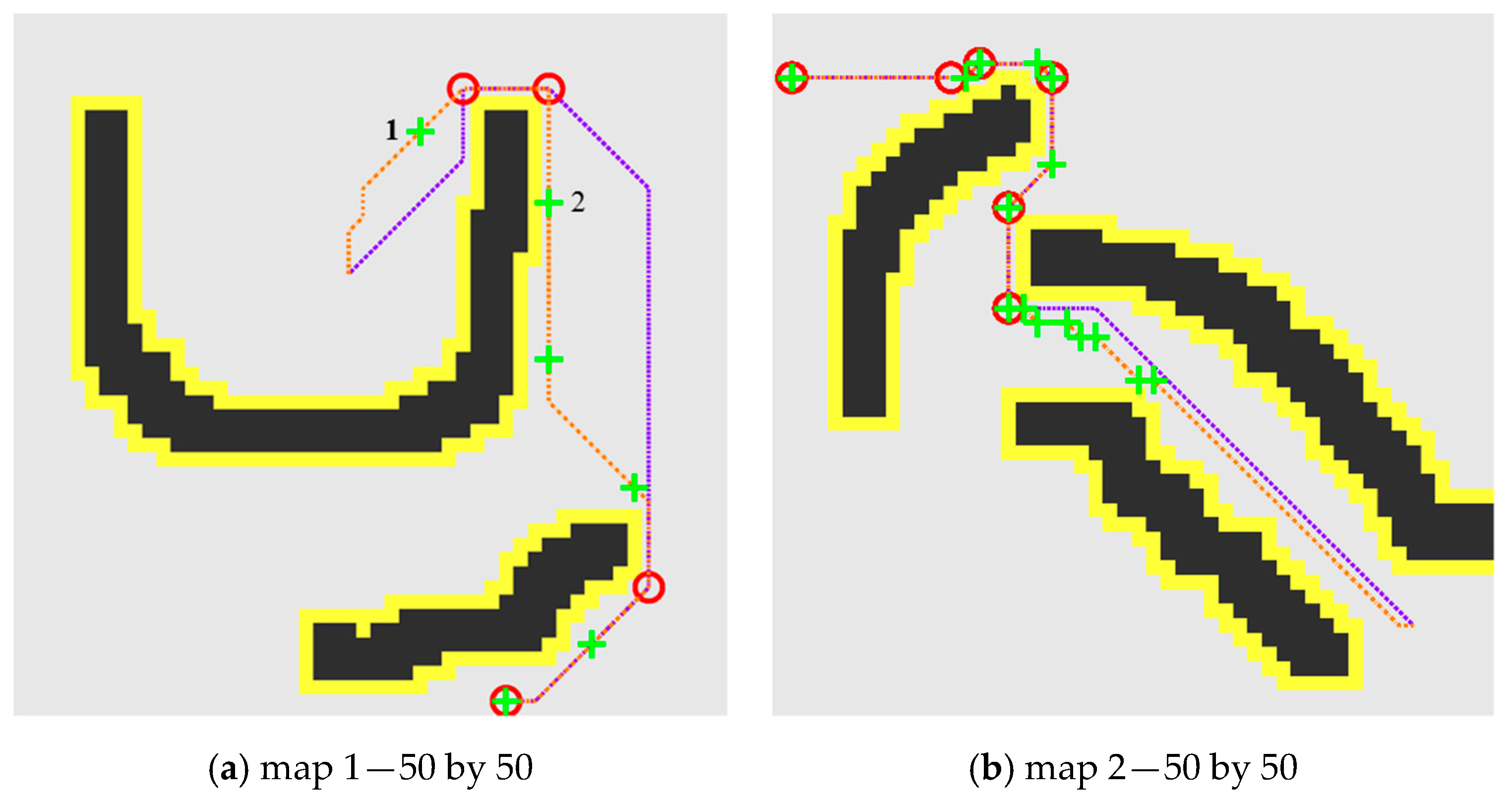
In Figure 7a, subgoals planned by A* are not placed at the exit of local minima due to ignoring the map topology, such as for example the local minimum caused by the concave canyon between subgoal 1 and subgoal 2. In Figure 7b, the number of subgoals of A* is over two times that of JPS-IA3C. Although the subgoals generated by A* cover all of the exits of local minima, they also include many unnecessary subgoals, which will hinder the ability to avoid moving obstacles. In conclusion, the subgoals planned by JPS-IA3C are essential waypoints that can help the motion controller handle the problem of local minima and simultaneously give full play to capabilities of the motion controller.
To avoid randomness, A* and JPS-IA3C are tested 100 times on large-scale maps (Figure 8), and the inflection points of optimal paths are regarded as subgoals of A*. First-move lags of A* include the time of planning optimal paths and finding subgoals by checking inflection points, while JPS-IA3C can directly finding subgoals without generating optimal paths. In Table 4, the first-move lags of A* are 271, 1309, and 860 times those of JPS-IA3C on these tested environments. Obviously, compared with A*, JPS-IA3C can more efficiently generate subgoals by the cached information about map topology and the canonical ordering way of search in JPS+ (P). Besides, the first-move lag of JPS-IA3C is below 1 millisecond on large-scale environments, which proves that the proposed approach can plan subgoals at low time costs to provide users with excellent experiences.
4.3. Evaluation of Local Motion Controlling
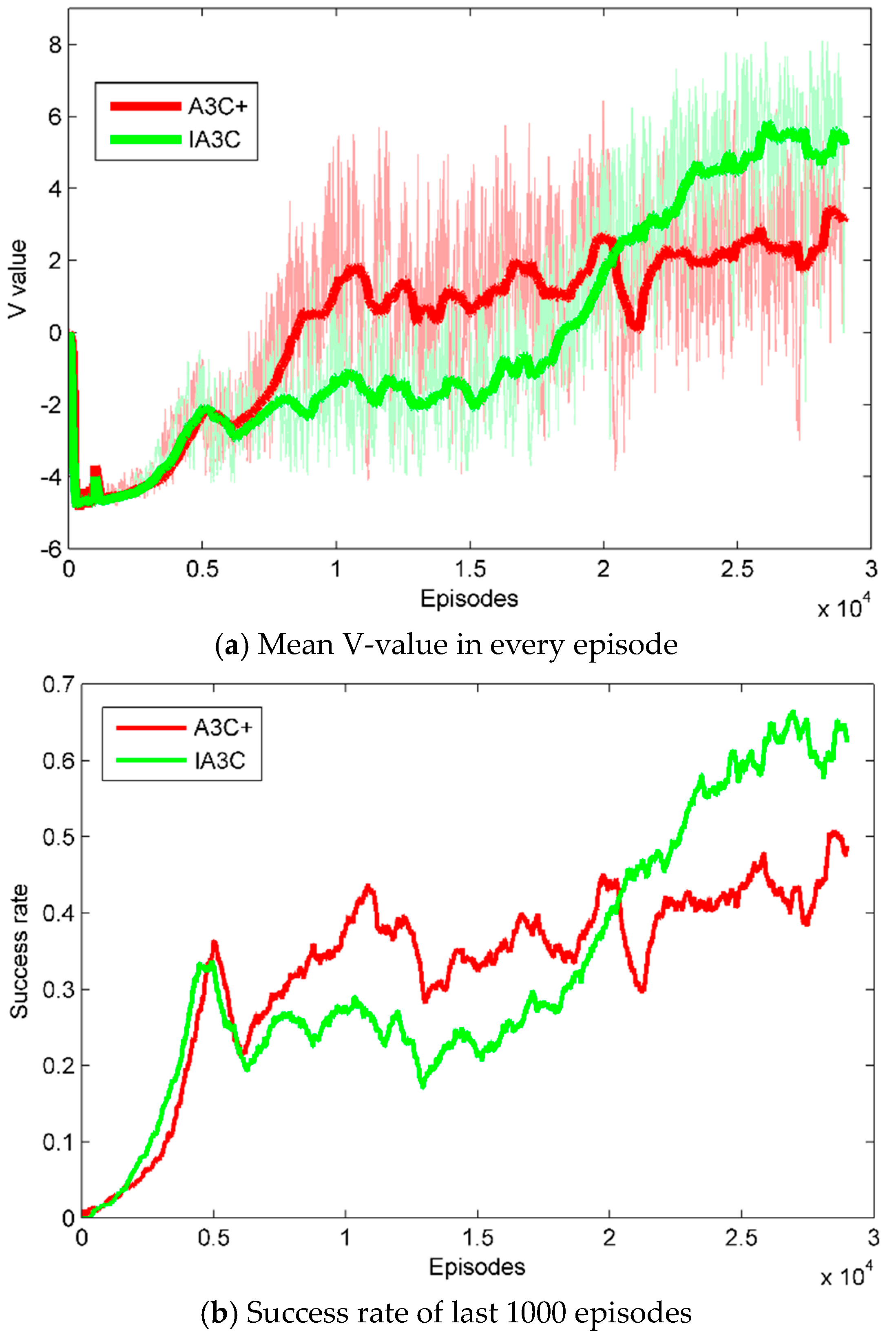
To evaluate the LSTM-based network, we compare IA3C with A3C+, which uses an FC layer to substitute an LSTM layer of IA3C’s network in the training process. State values denote the outputs of the critic-network, which can reflect the performances of learned policies [7]. Success rates are probabilities of accomplishing training tasks in the last 1000 episodes.
In Figure 8a, when the episode is less than 20,000, A3C+ performs better than IA3C. It demonstrates that A3C+ can learn reactive policies to deal with simple learning tasks that only require a robot to navigate for short distances while avoiding a few moving obstacles, and the learning efficiency of LSTM-based networks is slower than that of FC-based networks. When the complexity of learning tasks increases further (i.e., the episode increases to 20,000), the performance of IA3C is better than that of A3C+. It proves that the reactive policies generated by A3C+ only consider current observations, while IA3C can integrate current observations and abstract history information to learn more rational policies. Besides, modified curriculum learning can transfer experiences from learned tasks to new complex tasks, which is more suitable to accelerate the training efficiencies of LSTM-based networks. In Figure 8b, the data of success rates presents the same trend as that of the mean V-value, which further demonstrates the former conclusion.
To evaluate the effectiveness of the novel reward function framework, we remove individual reward shaping or single modified curriculum learning from the reward framework, but there is no way to converge. It shows that the proposed reward function framework can solve the problem of sparse reward and be beneficial for learning useful policies.
4.4. Performance on Large-Scale Navigation Tasks
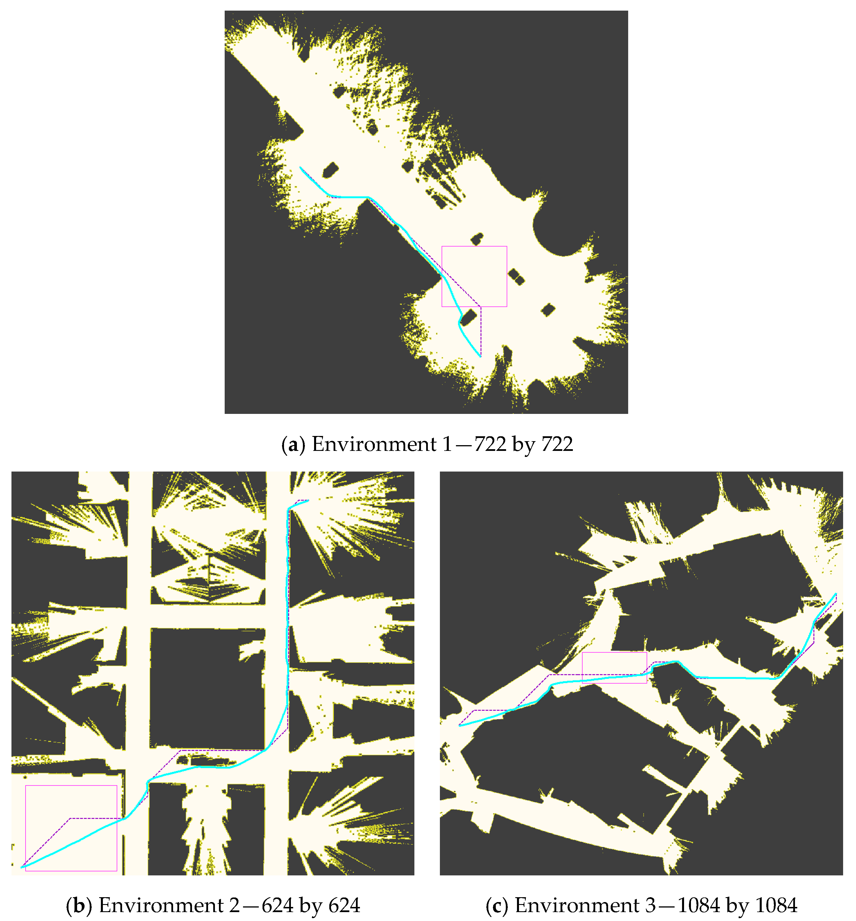
Finally, we evaluate the performance of JPS-IA3C on large-scale navigation tasks. JPS-A3C+ replaces IA3C with A3C+ in the proposed method. As shown in Figure 9, JPS-IA3C can navigate the nonholonomic robot with continuous control by dealing with both complex static obstacles and moving obstacles. Furthermore, navigation policies learned by JPS-IA3C have the notable generalization ability and can handle unseen tested environments that are almost three orders of magnitude larger than the training environment (Figure 6). We do not show trajectories generated by JPS-A3C+ for clear representation.
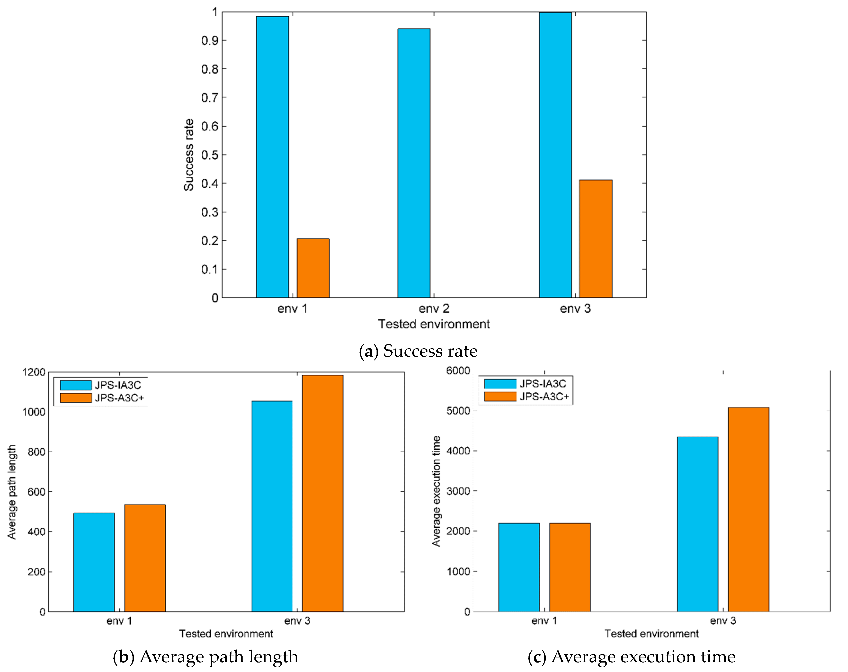
In Figure 10a, JPS-IA3C can achieve success rates of more than 94% in all of the tested environments and even 99.8% in environment 3, while the success rates of JPS-A3C+ are below 42% in all of the evaluations and even 0% in environment 2. Guided by the same subgoals, JPS-A3C+ only considers current observations and ignores hidden states (i.e., moving obstacles’ velocities and changes of map topology) from history observations, leading to collisions with complex static obstacles or moving obstacles. However, JPS-IA3C can use the LSTM-based network to construct accurate belief states by storing historical information over a certain length, which can handle environmental changes. In Figure 10b,c, compared with JPS-A3C+, JPS-IA3C can navigate robots in large-scale environments with shorter path lengths and less execution time, which concludes that constructing the LSTM-based network architecture can greatly improve the performance of the proposed algorithm by endowing the robot with certain memory.
5. Conclusions
In this paper, we proposed a novel hierarchical navigation approach to solving the problem of navigation in dynamic environments. It integrates a high-level path planner based on JPS+ (P) and a low-level motion controller based on an improved A3C (IA3C). JPS+ (P) can efficiently plan subgoals for the motion controller, which can eliminate first-move lag and address the challenge of the local minima trap. To meet the kinetic constraints and deal with moving obstacles, IA3C can learn near-optimal control policies to plan feasible trajectories between adjacent subgoals via continuous control. IA3C combines a modified curriculum learning and reward shaping to build a novel reward function framework, which can avoid learning inefficiency because of sparse reward. We additionally strengthen robots’ temporal reasoning about the environments by a memory-based network. These improvements make an IA3C controller converge faster and more adaptive to incomplete, noisy information caused by partial observability.
In simulation experiments, compared with A*, JPS-IA3C can plan more essential subgoals placed at the exit of local minima. Besides, JPS-IA3C’s first-move lag is between 271–1309 times shorter than A*’s on large-scale maps. Compared with A3C+ that remove IA3C’s memory-based network, IA3C can integrate current observation and abstract history information to achieve higher success rates and mean V-values in the training process. Finally, comparing JPS-A3C+, JPS-IA3C can navigate robots in unseen and large-scale environments with shorter path lengths and less execution time, with more than a 94% success rate.
In future work, we consider the more complex behaviors of moving obstacles in the real world. For example, in large shopping malls, people with different intentions can generate more complicated trajectories that cannot be predicted easily. The above problems can be solved by adding an external memory network [37] and feedback control mechanisms [38] into the network architectures of DRL agents, which estimates state-action values more accurately.
Author Contributions
J.Z. and L.Q. conceived and designed the paper structure and the experiments; J.Z. performed the experiments; Y.H., Q.Y., and C.H. contributed materials and analysis tools.
Funding
This work was sponsored by the National Science Foundation of Hunan Province (NSFHP) project 2017JJ3371, China.
Acknowledgments
The work described in this paper was sponsored by the National Natural Science Foundation of Hunan Province under Grant No. 2017JJ3371. We appreciate the fruitful discussion with the Sim812 group: Qi Zhang and Yabing Zha.
Conflicts of Interest
The authors declare no conflicts of interest. The founding sponsors had no role in the design of the study; in the collection, analysis, or interpretation of data; in the writing of the manuscript, or in the decision to publish the results.
References
- Mohanan, M.G.; Salgoankar, A. A survey of robotic motion planning in dynamic environments. Robot. Auton. Syst. 2018, 100, 171–185. [Google Scholar] [CrossRef]
- Mercorelli, P. Using Fuzzy PD Controllers for Soft Motions in a Car-like Robot, Advances in Science. Technol. Eng. Syst. J. 2018, 3, 380–390. [Google Scholar]
- Lavalle, S.M. Rapidly-exploring random trees: Progress and prospects. In Proceedings of the 4th International Workshop on Algorithmic Foundations of Robotics, Hanover, Germany, 16–18 March 2000. [Google Scholar]
- Kavraki, L.E.; Švestka, P.; Latombe, J.C.; Overmars, M.H. Probabilistic roadmaps for path planning in high-dimensional configuration spaces. IEEE Trans. Robot. Autom. 1994, 12, 566–580. [Google Scholar] [CrossRef]
- Van Den Berg, J.; Guy, S.J.; Lin, M.; Manocha, D. Reciprocal nbody collision avoidance. In Robotics Research; Springer: Berlin/Heidelberg, Germany, 2011; pp. 3–19. [Google Scholar]
- Lecun, Y.; Bengio, Y.; Hinton, G. Deep learning. Nature 2015, 521, 436. [Google Scholar] [CrossRef] [PubMed]
- Mnih, V.; Kavukcuoglu, K.; Silver, D.; Rusu, A.; Veness, J.; Bellemare, M.G.; Graves, A.; Riedmiller, M.; Fidjeland, A.K.; Ostrovski, G.; et al. Human-level control through deep reinforcement learning. Nature 2015, 518, 529. [Google Scholar] [CrossRef] [PubMed]
- Lillicrap, T.P.; Hunt, J.; Pritzel, A.; Heess, N.; Erez, T.; Tassa, Y.; Silver, D.; Wierstra, D. Continuous control with deep reinforcement learning. arXiv, 2016; arXiv:1509.02971. [Google Scholar]
- Mirowski, P.; Pascanu, R.; Viola, F.; Soyer, H.; Ballard, A.J.; Banino, A.; Denil, M.; Goroshin, R.; Sifre, L.; Kavukcuoglu, K.; et al. Learning to Navigate in Complex Environments. arXiv, 2016; arXiv:1611.03673. 2016. [Google Scholar]
- Mirowski, P.; Grimes, M.; Malinowski, M.; Hermann, K.M.; Anderson, K.; Teplyashin, D.; Simonyan, K.; Zisserman, A.; Hadsell, R. Learning to Navigate in Cities Without a Map. arXiv, 2018; arXiv:1804.00168. [Google Scholar]
- Zhu, Y.; Mottaghi, R.; Kolve, E.; Lim, J.J.; Gupta, A.; Fei-Fei, L.; Farhadi, A. Target-driven visual navigation in indoor scenes using deep reinforcement learning. In Proceedings of the International Conference on Robotics and Automation, Singapore, 29 May–3 June 2017; pp. 3357–3364. [Google Scholar]
- Mnih, V.; Badia, A.P.; Mirza, M.; Graves, A.; Lillicrap, T.; Harley, T.; Silver, D.; Kavukcuoglu, K. Asynchronous methods for deep reinforcement learning. In Proceedings of the International Conference on Machine Learning, New York, NY, USA, 19–24 June 2016; pp. 1928–1937. [Google Scholar]
- Hausknecht, M.J.; Stone, P. Deep Recurrent Q-Learning for Partially Observable MDPs. arXiv, 2015; arXiv:1507.06527. [Google Scholar]
- Rabin, S.; Silva, F. JPS+ An Extreme A* Speed Optimization for Static Uniform Cost Grids. In Game AI Pro, 2nd ed.; Rabin, S., Ed.; CRC Press: Boca Raton, FL, USA, 2015; Volume 3, pp. 131–143. ISBN 9781482254792. [Google Scholar]
- Otte, M.; Frazzoli, E. RRT-X: Real-time motion planning/replanning for environments with unpredictable obstacles. In Proceedings of the International Workshop on Algorithmic Foundations of Robotics (WAFR), Istanbul, Turkey, 3–5 August 2014. [Google Scholar]
- Kallman, M.; Mataric, M.J. Motion planning using dynamic roadmaps. In Proceedings of the IEEE International Conference on Robotics and Automation (ICRA), New Orleans, LA, USA, 26 April–1 May 2004; pp. 4399–4404. [Google Scholar]
- Chen, C.; Seff, A.; Kornhauser, A.; Xiao, J. Deepdriving: Learning affordance for direct perception in autonomous driving. In Proceedings of the IEEE International Conference on Computer Vision, Santiago, Chile, 7–13 December 2015; pp. 2722–2730. [Google Scholar]
- Gao, W.; Hsu, D.; Lee, W.S.; Shen, S.; Subramanian, K. Intention-Net: Integrating Planning and Deep Learning for Goal-Directed Autonomous Navigation. arXiv, 2017; arXiv:1710.05627. [Google Scholar]
- Pfeiffer, M.; Schaeuble, M.; Nieto, J.; Siegwart, R.; Cadena, C. From perception to decision: A data-driven approach to end-to end motion planning for autonomous ground robots. arXiv, 2016; arXiv:1609.07910. [Google Scholar]
- Guo, Y.; Liu, Y.; Oerlemans, A.; Lao, S.; Wu, S.; Lew, M.S. Deep learning for visual understanding: A review. Neurocomputing 2016, 187, 27–48. [Google Scholar] [CrossRef]
- Tai, L.; Zhang, J.; Liu, M.; Boedecker, J.; Burgard, W. A Survey of Deep Network Solutions for Learning Control in Robotics: From Reinforcement to Imitation. arXiv, 2016; arXiv:1612.07139. [Google Scholar]
- Tai, L.; Paolo, G.; Liu, M. Virtual-to-real deep reinforcement learning: Continuous control of mobile robots for mapless navigation. In Proceedings of the 2017 IEEE/RSJ International Conference on Intelligent Robots and Systems (IROS), Vancouver, BC, Canada, 24–28 September 2017. [Google Scholar]
- Chen, Y.F.; Everett, M.; Liu, M.; How, J.P. Socially aware motion planning with deep reinforcement learning. arXiv, 2017; arXiv:1703.08862. [Google Scholar]
- Kato, Y.; Kamiyama, K.; Morioka, K. Autonomous robot navigation system with learning based on deep Q-network and topological maps. In Proceedings of the IEEE/SICE International Symposium on System Integration, Taipei, Taiwan, 11–14 December 2017; pp. 1040–1046. [Google Scholar]
- Faust, A.; Oslund, K.; Ramirez, O.; Francis, A.; Tapia, L.; Fiser, M.; Davidson, J. PRM-RL: Long-range Robotic Navigation Tasks by Combining Reinforcement Learning and Sampling-Based Planning. In Proceedings of the International Conference on Robotics and Automation, Brisbane, QLD, Australia, 21–25 May 2018; pp. 5113–5120. [Google Scholar]
- Zuo, L.; Guo, Q.; Xu, X.; Fu, H. A hierarchical path planning approach based on A* and least-squares policy iteration for mobile robots. Neurocomputing 2015, 170, 257–266. [Google Scholar] [CrossRef]
- Canny, J. The Complexity of Robot Motion Planning; MIT Press: Cambridge, MA, USA, 1988. [Google Scholar]
- Bulitko, V.; Lee, G. Learning in real-time search: A unifying framework. J. Artif. Intell. Res. 2006, 25, 119–157. [Google Scholar] [CrossRef]
- Zaremba, W.; Sutskever, I. Learning to Execute. arXiv, 2014; arXiv:1410.4615. [Google Scholar]
- Sutton, R.S.; Barto, A.G. Reinforcement Learning: An Introduction, 2nd ed.; MIT Press: Boston, MA, USA, 2018. [Google Scholar]
- Lau, B.; Sprunk, C.; Burgard, W. Efficient grid-based spatial representations for robot navigation in dynamic environments. Robot. Autom. Syst. 2013, 61, 1116–1130. [Google Scholar] [CrossRef]
- Harabor, D.; Grastien, A. Improving jump point search. In Proceedings of the International Conference on Automated Planning and Scheduling, Portsmouth, NH, USA, 21–26 June 2014; pp. 128–135. [Google Scholar]
- Karkus, P.; Hsu, D.; Lee, W.S. QMDP-Net: Deep Learning for Planning under Partial Observability. arXiv, 2017; arXiv:1703.06692. [Google Scholar]
- Ravankar, A.; Ravankar, A.A.; Kobayashi, Y.; Takanori, E. SHP: Smooth Hypocycloidal Paths with Collision-Free and Decoupled Multi-Robot Path Planning. Int. J. Adv. Robot. Syst. 2016, 13, 133. [Google Scholar] [CrossRef] [Green Version]
- Bengio, Y.; Louradour, J.; Collobert, R.; Weston, J. Curriculum learning. In Proceedings of the 26th Annual International Conference on Machine Learning, ICML 2009, Montreal, QC, Canada, 14–18 June 2009. [Google Scholar]
- Garcia-Cruz, X.M.; Sergiyenko, O.Y.; Tyrsa, V.; Rivas-Lopez, M.; Hernandez-Balbuena, D.; Rodriguez-Quiñonez, J.C.; Basaca-Preciado, L.C.; Mercorelli, P. Optimization of 3D laser scanning speed by use of combined variable step. Opt. Lasers Eng. 2014, 54, 141–151. [Google Scholar] [CrossRef]
- Parisotto, E.; Salakhutdinov, R. Neural Map: Structured Memory for Deep Reinforcement Learning. arXiv, 2017; arXiv:1702.08360. [Google Scholar]
- Oh, J.; Chockalingam, V.; Singh, S.; Lee, H. Control of memory, active perception, and action in minecraft. arXiv, 2016; arXiv:1605.09128. [Google Scholar]
Figure 1.
Schematic diagram of the tracked robot. Gray dash-dotted lines denote the senor lines of the robot.
Figure 1.
Schematic diagram of the tracked robot. Gray dash-dotted lines denote the senor lines of the robot.

Figure 2.
Flowchart of the Jump Point Search improved Asynchronous Advantage Actor-Critic (JPS-IA3C) method.
Figure 2.
Flowchart of the Jump Point Search improved Asynchronous Advantage Actor-Critic (JPS-IA3C) method.

Figure 3.
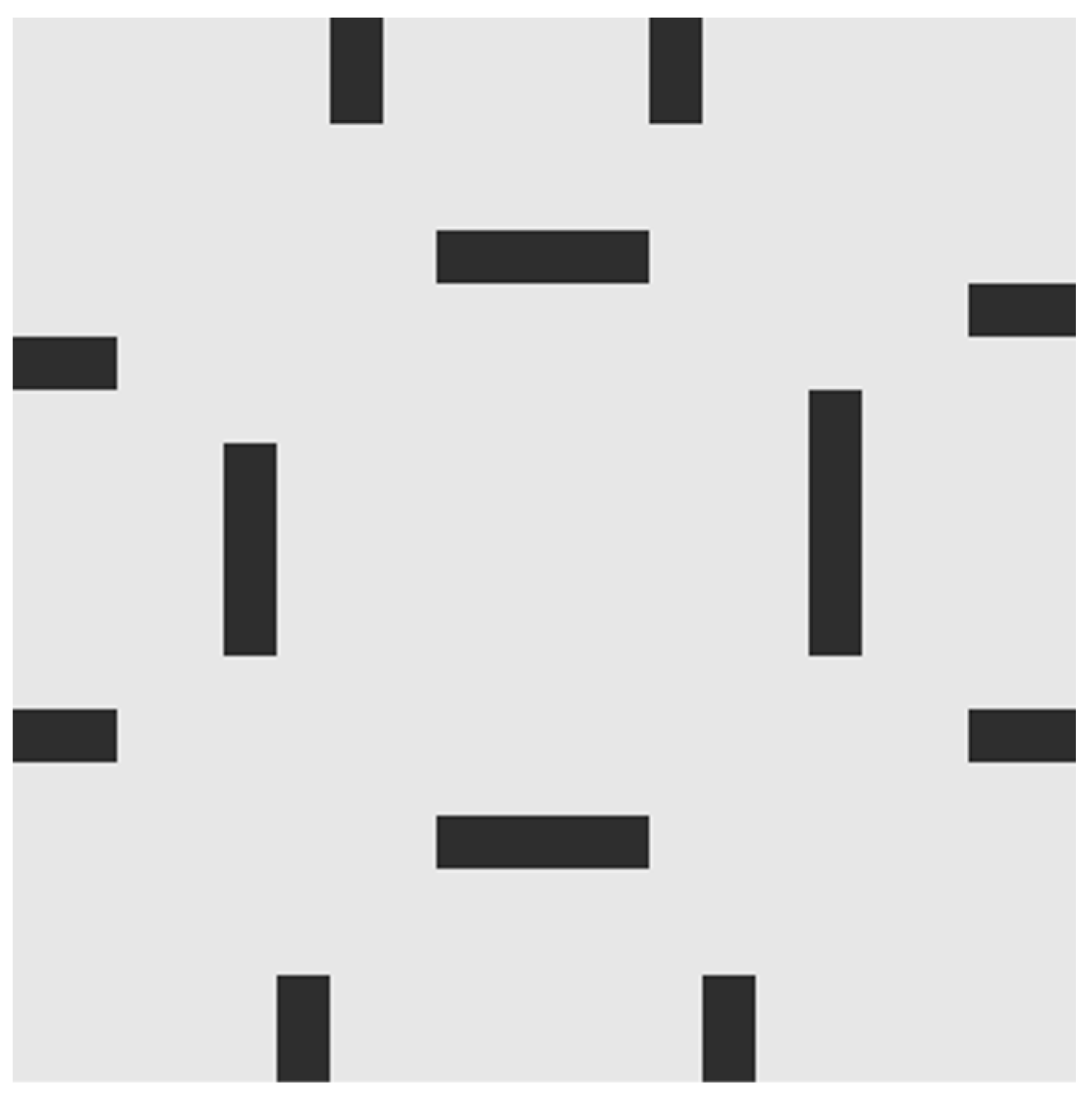
A graphical representation of how Jump Point Search+ (Prune) (JPS+ (P)) preprocesses an initially known grid-based map and what the paths that it plans look like. (a) An original map in which the white and black cells are unblocked and blocked locations, respectively. (b) Gray cells denote warning areas. (c) Jump points are marked as red. (d) Green lines denote an optimal path planned by JPS+ (P).
Figure 3.
A graphical representation of how Jump Point Search+ (Prune) (JPS+ (P)) preprocesses an initially known grid-based map and what the paths that it plans look like. (a) An original map in which the white and black cells are unblocked and blocked locations, respectively. (b) Gray cells denote warning areas. (c) Jump points are marked as red. (d) Green lines denote an optimal path planned by JPS+ (P).

Figure 4.
The flowchart of Asynchronous Advantage Actor-Critic (A3C).

Figure 5.
The network structure of IA3C.

Figure 6.
Training environment—20 by 20.

Figure 7.
(a–b) Orange lines denote paths planned by A*, and purple lines denote paths generated by the path planner in JPS-IA3C. Small red circles denote subgoals planned by JPS-IA3C. Yellow regions denote warning areas. (a) A* find subgoals (i.e., green crosses) by sampling optimal paths at fixed intervals. (b) A* plans subgoals (i.e., green crosses) through taking the inflection points of optimal paths.

Figure 8.
The performances of IA3C and A3C+ in the training phase.

Figure 9.
(a–c) Given the start position and the goal position, the purple line is the path planned by the Jump Point Search+ (Prune) (JPS+ (P)), and the blue line is the trajectory generated by JPS-IA3C. Black regions are unpassable, while light white regions are traversable for robots. Yellow regions close to obstacles denote warning areas. Moving obstacles appear in pink square areas, where there are 30 random moving obstacles.

Figure 10.
We generate 500 navigation tasks in each tested environment (in sum 1500) whose starting and goal points are randomly chosen. The distance between the initial starting and goal position is greater than half of the width of the environment. (a) Success rate denotes the probability of successfully finishing tasks. (b) Path length denotes the traveling length between the starting and goal position. (c) Execution time denotes the total execution time for the motion controller.


Table 1.
Definitions of the Partially Observable Markov Decision Process (POMDP).
| Observations | () | |
| Actions | ||
| Reward | +10 | if |
| −5 | if | |
| 0 | else | |
Table 2.
Learning plan of modified curriculum learning.
| Number of Obstacles | Distance | Training Episodes |
|---|---|---|
| 1 | 3 | 5000 |
| 2 | 5 | 7000 |
| 3 | 9 | 8000 |
| 3 | 13 | 9000 |
Table 3.
Reward shaping.
| Reward | +10 | if |
| −5 | if | |
| else |
Table 4.
First-Move Lag of A* and JPS-IA3C.
| Method | Environment 1 (ms) | Environment 2 (ms) | Environment 3 (ms) |
|---|---|---|---|
| JPS-IA3C | 0.097 | 0.134 | 0.230 |
| A* | 26.287 | 175.36 | 197.71 |
The first-move lag denotes the amount of planning time the robot takes before deciding on the first move (i.e., time of finding subgoals).
© 2019 by the authors. Licensee MDPI, Basel, Switzerland. This article is an open access article distributed under the terms and conditions of the Creative Commons Attribution (CC BY) license (http://creativecommons.org/licenses/by/4.0/).
Share and Cite
MDPI and ACS Style
Zeng, J.; Qin, L.; Hu, Y.; Yin, Q.; Hu, C. Integrating a Path Planner and an Adaptive Motion Controller for Navigation in Dynamic Environments. Appl. Sci. 2019, 9, 1384. https://0-doi-org.brum.beds.ac.uk/10.3390/app9071384
AMA Style
Zeng J, Qin L, Hu Y, Yin Q, Hu C. Integrating a Path Planner and an Adaptive Motion Controller for Navigation in Dynamic Environments. Applied Sciences. 2019; 9(7):1384. https://0-doi-org.brum.beds.ac.uk/10.3390/app9071384
Chicago/Turabian StyleZeng, Junjie, Long Qin, Yue Hu, Quanjun Yin, and Cong Hu. 2019. "Integrating a Path Planner and an Adaptive Motion Controller for Navigation in Dynamic Environments" Applied Sciences 9, no. 7: 1384. https://0-doi-org.brum.beds.ac.uk/10.3390/app9071384
Note that from the first issue of 2016, this journal uses article numbers instead of page numbers. See further details here.