Fashion Product Classification through Deep Learning and Computer Vision


IMP Lab, Department of Engineering and Architecture, University of Parma, 43121 Parma, Italy
*
Author to whom correspondence should be addressed.
Appl. Sci. 2019, 9(7), 1385; https://0-doi-org.brum.beds.ac.uk/10.3390/app9071385
Submission received: 13 February 2019
/
Revised: 12 March 2019
/
Accepted: 23 March 2019
/
Published: 2 April 2019
(This article belongs to the Section Computing and Artificial Intelligence)
Abstract
:Featured Application
This work has its application in the data analysis and classification of clothing products, into the fashion workflow of Adidas AG™.
Abstract
Visual classification of commercial products is a branch of the wider fields of object detection and feature extraction in computer vision, and, in particular, it is an important step in the creative workflow in fashion industries. Automatically classifying garment features makes both designers and data experts aware of their overall production, which is fundamental in order to organize marketing campaigns, avoid duplicates, categorize apparel products for e-commerce purposes, and so on. There are many different techniques for visual classification, ranging from standard image processing to machine learning approaches: this work, made by using and testing the aforementioned approaches in collaboration with Adidas AG™, describes a real-world study aimed at automatically recognizing and classifying logos, stripes, colors, and other features of clothing, solely from final rendering images of their products. Specifically, both deep learning and image processing techniques, such as template matching, were used. The result is a novel system for image recognition and feature extraction that has a high classification accuracy and which is reliable and robust enough to be used by a company like Adidas. This paper shows the main problems and proposed solutions in the development of this system, and the experimental results on the Adidas AG™ dataset.
1. Introduction
In fashion industries, obtaining a visual analysis of the overall production is a key aspect, both in developing marketing strategies and for helping fashion designers in the creative workflow of new products. As a first important step in order to proceed with a visual analysis, the various outcomes of the designers’ work must be collected and categorized. This applies especially if there are many different designer teams which are employed with outsourcing contracts, and located all around the world, as it usually happens with large companies. In particular, in Adidas AG™, the designers’ production comprises a consistent number of images which represent a very large variety of products, from clothing to footwear. Moreover, these works are usually independent from each other. Then, articles are of different types and come from different sources, but their characteristics must be analyzed and classified as a whole by data experts and analysts. Hence, a significant step in visual analysis is recognizing, classifying, and extracting features directly from final images or 3D-renderings of products, collected before the actual fabrication of the clothing. Categorizing apparel products is also useful for e-commerce purposes, as well as for avoiding duplicates, ranking product types, or doing statistical analysis [1].
The categorization of apparel products was, until now, manually performed by Adidas teams, since it requires both domain expertise and a comprehensive knowledge over the range of products. Such a manual classification is an error-prone task that may cause incorrect results, misleading the subsequent visual analysis, and which also requires too much time. As a matter of fact, over the years, the number of produced articles has grown significantly, and, currently, Adidas teams invent ~20 k different articles per season (twice a year). For all these products, about two dozen main attributes (or categories) were identified by Adidas data experts, such as the presence and position of logos or the three-stripes, which is the primary color, the presence of prints or clothing patterns, and so on. Each of these categories takes values in a different domain, and ranges across a set of possible classes. As expected, manually performing the classification of attributes for each article has become an unfeasible task. Due to the large amount of data, and the diversity of the source of images, the task of classifying and recognizing features of clothing images is not only hard to perform manually, but, at the same time, it is also difficult to automate properly. A subset of seven key attributes were chosen, which we will call features in the next, namely, (i) logo type and size, (ii) three-stripes presence and colors, (iii) three main colors palette, (iv) prints and patterns, (v) neck shape, (vi) sleeve shape, and (vii) material of the clothing. These features are the most important both for business reasons (e.g., detecting logos in clothing is a fundamental information for a brand), and for their significance in identifying a particular garment, so as to avoid or substantially reduce duplicates or similar products. The characteristics of each feature and the reasons for their importance are detailed later in the paper.
The core idea is to automate the classification process of these seven features by using machine learning techniques and computer vision, but many aspects in such a task raise concrete research problems. In fact, each clothing feature could eventually require a different method of classification, spacing from segmentation [2,3], image retrieval [4], to machine learning techniques, such as deep learning [5,6,7,8]. These algorithms must be applied to the under-investigated area of fashion, and must be refined for the specific domain. In addition, the automatization must have an accuracy comparable to manual methods in order to be useful for business purposes. Thus, the problem of automatic classification of apparel features turned out to be a challenging application of computer vision and machine learning techniques. The purpose of this paper is to describe a work that was developed by the authors to offer an effective solution to the aforementioned problem, by means of a computer vision software system, and to discuss challenges that arise in the development of that system, feature by feature.
The paper is structured as follows. First, a review on the state-of-the-art of the used techniques and a discussion on related works is done in Section 2. Then, Section 3 shows an overview of the developed system. In Section 4 and Section 5, feature extraction is described in detail, with an emphasis on logo detection. Experimental results are provided in Section 6, and, finally, a discussion of main achievements and future works concludes the paper.
2. Related Works
As briefly explained in the introduction, feature extraction from final images of products requires different methods and techniques, depending on which feature to extract. Two main fields are usually investigated, namely, the image classification (or recognition), and the detection of objects in the image. In the following, a brief outline of the major contributions in image classification, object localization and detection is provided. An outline of this related works section could be found in another authors’ work [9], which presents also a preliminary discussion on this project. However, the study of the state-of-the-art, as well as the development of the described system and the experimental results are substantially enhanced and expanded in this paper.
Many feature extraction tasks, such as recognizing logos and locating them, or detecting prints and clothing patterns, are sub-problems of the object detection task. Object detection is a well-known computer vision task [10] that is employed in many application contexts, such as face detection [11], visual search engines [1], image analysis [12], self-driving cars [13], and so on. A very popular competition which poses the object detection as a central challenge is the ImageNet competition [14,15]. A large dataset is provided, and the purpose of the competition is finding multiple objects for each image and classifying them properly. In particular, the candidate system must retrieve the five best-matching categories of objects in the input image, putting bounding boxes around recognized objects.
Early object detection algorithms were based on integral images [11,16], and feature descriptors [17,18]. In detail, the work of Viola and Jones [11] is a fast face detection algorithm based on integral images and that uses a learning algorithm. Such an approach proved successful, and showed the potentialities of computer vision in real world applications. Nevertheless, face detection is only a narrowed type of object detection, and an improvement is necessary in order to apply it in a more generic context. Then, Dalal and Triggs [17] enhanced previous methods by proposing feature descriptors called Histograms of Oriented Gradients (HOG) for pedestrian detection. The problem with such a method is the same: generalization to other domains, such as fashion, is hardly obtainable. Other descriptors are shown in the work of Lowe [18] that presents a method for image feature generation called Scale Invariant Feature Transform (SIFT), and Bay et al. [19] that propose SURF (Speeded-Up Robust Features), a detector and descriptor which is both scale and rotation invariant, and that speeds up detection using integral images. Nowadays, such approaches are useful in very specialized contexts, and in general—in the task of object detection—they are outperformed by more accurate learning algorithms.
As a matter of fact, most successful approaches are based on deep learning techniques, such as Convolutional Neural Networks (CNNs or ConvNets) [5,6,20,21,22,23,24,25,26], that achieve good results in detecting multiple objects, even of various classes, in a given image. Overfeat [24] is an early work that uses multi-scale sliding windows and deep learning (CNNs) for object detection. An enhancement of the CNN approach is a method developed by Girshick et al. [20], called Regions with CNN features (R-CNN), which uses a three-stage algorithm that is not entirely based on deep learning. As a matter of fact, the first step is a region proposal, while the second step uses a CNN for feature extraction. For the final classification, a SVM classifier is used. R-CNN significantly enhanced object detection w.r.t. training a CNN from scratch, but it still had many problems during the training phase. Girshick [21] then additionally proposed an improvement of R-CNN that deals with the speed and training problems of the previous model. Such an improvement was called Fast R-CNN, and conversely to R-CNN, it has a pure deep learning paradigm: it employs CNNs also for classification, and uses the Region of Interest (RoI) Pooling. As a further enhancement of the R-CNN approach, a Region Proposal Network (RPN) was added to the Fast R-CNN method. This development is called Faster R-CNN [23]. The Region-based Fully Convolutional Networks (R-FCN) [6] is somehow similar to Faster R-CNN, since it uses the same architecture, but relying also on CNNs. A work that substantially helps at developing our feature extractor system is the VGG19 network [8], the 2014 winner of the ImageNet challenge in the localization task. VGG19 has a simple architecture which consists of a plain chain of layers, and it owes its good performances—comparable to other more complicated networks—to the use of much more memory and to a slower evaluation time. Its simple structure makes it valuable for our work. Recently, a novel and deep learning based approach was proposed by Redmon et al. [5]. The project is called YOLO (You Only Look Once), and it is currently under development [27]. Another recent approach, named SSD (Single Shot Multibox Detector) [25], is based on a single deep neural network, as for YOLO, and it achieved better results and speed than it. The second enhancement of YOLO is YOLO9000 [22], and a new version was also released in 2018 [26].
As an important drawback, deep learning requires huge amount of data. This is due to two main reasons: first, a neural network with many layers has a lot of parameters (weights and biases), which could be properly trained only by using a high number of samples; second, a large and diverse dataset helps at preventing the overfitting of such a network. Moreover, using a supervised approach also requires data to be labeled. Unfortunately, there is a scarcity of labeled datasets from apparel industries, and all the previously detailed deep learning techniques suffer from these disadvantages [28]. Public datasets of colored images at an acceptable resolution for deep learning, such as the ImageNet one, have a high number of classes which have nothing to do with the fashion industry, and the Fashion-MNIST [29] dataset, which could appear more appropriate for the application domain, consists of very small grayscale images () divided in 10 classes, which are not sufficient for our purposes.
In this paper, we approach the problem of lack of data with two different methods. One is the use of Pearson Correlation Coefficient (PCC) [30] to perform a masked template matching. This method shows, in specific cases (e.g., recognition of small logos), more accurate results than a CNN approach. The other one is the fine-tuning of a pre-trained CNN, i.e., a method to specialize a neural model on personalized data by only training the last layers of the network. In this last case, a pre-processing step of data-augmentation [28] is also needed.
Other features require a more standard computer vision approach, since they are either based on the geometric properties of the garment contours (e.g., stripes recognition), or they involve the calculation of distances in color spaces. First, a border-following algorithm to retrieve the contour of the shape of the garment is needed. A great method for such a task is described in [31]. Then, the natural choice for reducing line shapes to a compact form is to apply a thinning algorithm [32]. Thinning variants are well described in the review [33]. Nevertheless, thinning algorithms suffer from a problem called skeletonization bias [33]. The unwanted bias effect arises when thinning is applied to strongly-concave angles. As described by Chen [34], the bias effect appears when the shape to be thinned has a contour angle steeper than 90 degrees. The original proposal in [34] is based, first, on the detection of steep angles and, then, on the application of a custom local erosion specifically designed to eliminate the so-called “hidden deletable pixels”. In the work [35], an overview of line extraction and vectorization of sketches is shown, and in particular a solution to the skeletonization bias problem is proposed. The same research topic has been explored in the work by Chen et al. [36], which showed remarkable results in the task of disambiguating parallel, almost touching, strokes, which is a very useful property in the sketch analysis domain. A great line extraction and thinning is of fundamental importance for reasoning on geometric characteristics of clothing, in terms of parallel or perpendicular strokes. A line extraction and thinning approach was used in this work for the recognition of the Adidas three-stripes.
3. System Overview
The proposed system aims at automatizing the classification of seven features, as previously mentioned. In the following, there is a more detailed description of these features:
- Logo size and type. There are three main Adidas logos, namely, the original “Badge Of Sports” (BOS), the trefoil, and the linear one (as shown in Figure 1); each of them could appear as a small, medium or large logo;
- Three-stripes presence and colors. A mark that is characteristic of Adidas consists of three equidistant bands of the same color, typically on the sleeves of shirts or on the side of pants. The three-stripes can be contrasted or tonal: this refers to the difference between their color and the color of the background;
- Three main colors palette. For each article, a maximum of three visible colors should be extracted, ordered by their importance, and the percentage of the area covered by such colors should be provided;
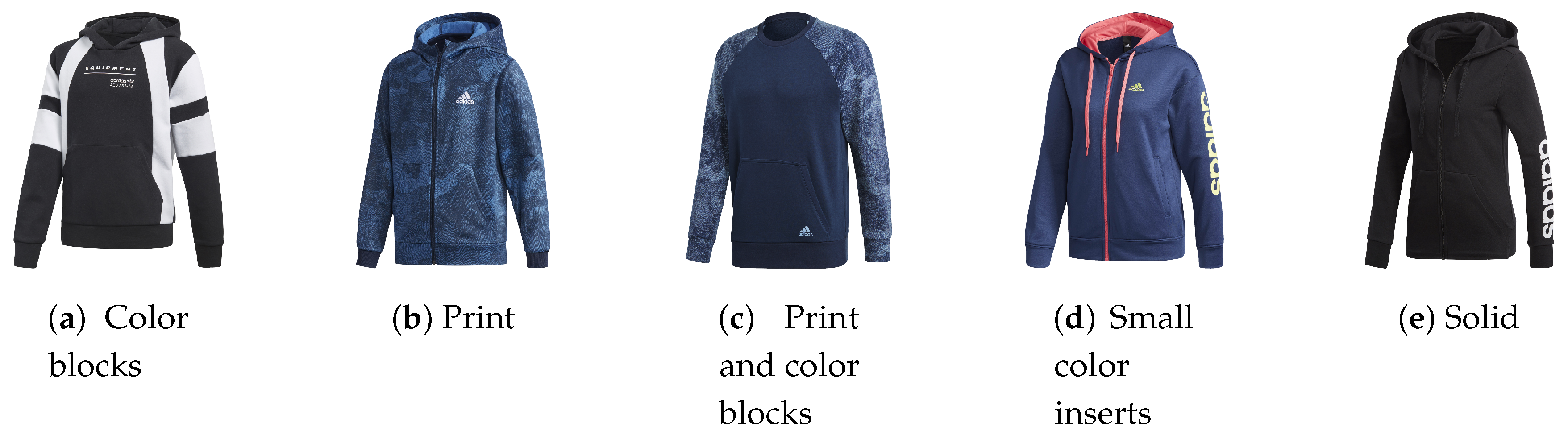
- Prints and clothing patterns. Besides colors, there could be prints over the clothing, textured fabrics, or geometric patterns: this is called the main-execution of the article (examples are shown in Figure 2);
- Neck shape. The type of the collar of a jacket, a sweatshirt or a shirt can be classified in major categories, like U-neck, V-neck, hooded, bomber, and so on (illustrated in Figure 3);
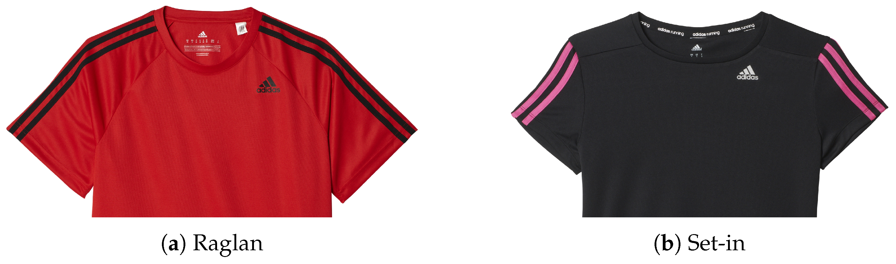
- Sleeves shape. Adidas teams need to differentiate between “raglan” and “set-in” sleeves, i.e., the shape of the junction between sleeves and body of the garment, as in Figure 4;
- Material of the clothing. Clothes have a lot of fabric types, but at this stage (recognition from final renderings), only cotton, (generic) synthetic, and viscose fabrics have to be distinguished.
Some preliminary considerations help at understanding the main problems that have to be faced in the development of the system. Thus, when choosing the right method for each feature, the following points have been carefully taken in account:
- The complete dataset that Adidas teams provide us with consists of about 11k images, where articles could be duplicated (e.g., for many of them, clothes back-view and front-view are depicted separately). The great majority of these images are unlabeled, i.e., no classification is provided for the aforementioned seven features. Not considering duplicates, only 2616 images of this dataset were manually labeled by Adidas data experts, thus indicating the correct classification of each feature. This small portion of 2616 images of the dataset was used as ground truth for all the proposed algorithms.
- Classifications are sometimes difficult to perform even by a human observer, since they depend on very small details, or not well-defined classes: e.g., recognizing the material (synthetic, cotton, or viscose) of a garment only from its rendering image is very hard;
- For some features, classes range in a high variety of values, as for color names, and examples for each class are very few; moreover, having many classes could mean that inter-class differences are small, and this may lead to inaccurate results.
For these reasons, a different module was developed for each feature. Features (1)–(3) have been approached with classic image processing methods, while the others have been approached with deep learning. As an exception, the logo search was also reinforced by using a deep network for certain types of logos. In Figure 5, a detailed schema illustrates the structure of the system. Note that the list of output classes in Figure 5 is not an exhaustive one, since in all cases the search could either fail, returning a NONE output (e.g., no logos have been found in the image), or may not make sense, returning a NOT APPLICABLE output (e.g., no neck shape has to be found in case the image depicts pants). In addition, implementation details are outlined in the following, but they are not shown in the diagram, for the sake of clarity.
Input images are colored 3D-renderings or pictures of the final products. The provided dataset consists of about 11k images depicting T-shirts, sweatshirts, short and long pants, and jackets, of which only 2616 are labeled and not duplicate. The diversity of such images is very high, meaning that the search for a feature may or may not make sense, depending on the input image given. Nevertheless, images are comparable in size, although they do not always have the same dimension (small products are stretched and big ones are shrunk). As another common point, the front-view or back-view of the clothing to be analyzed is the only picture in the image, with no noise in the background. Colors are well visible (brightness is uniform) and as realistic as a photo. An initial step of preprocessing is needed, for each image. Such a little prior step is necessary for each feature.
The preprocessing phase consists of two main operations: the extraction of the shape of the garment in the image, separating it from the background, and the size normalization of the article. Only when needed, the clothing depicted in the image must be preliminary classified as a shirt or a sweatshirt, a jacket, short or long pants, bra or tank tops, and so on. Well-known image processing algorithms are used in this preprocessing phase, as well as some low-level heuristics. The shape of the article is treated as a binary image to be passed as additional informative content in the following steps of the elaboration. Its extraction is an easy task, given the absence of noisy backgrounds. Size normalization is based on the waist size of the product. This normalization aims, in fact, at producing a homogeneous dataset for future computation. The objective is achieved by detecting the waist in various types of clothing—usually placed in the middle of the image—and rescaling the image according to a given waist size to be matched. The article type classification is made by training a deep neural network, using a supervised approach, where images are labeled as shirts, pants, tops, and sweatshirts. Then, the input image enters into an “executor” module, whose only purpose is the launch of one, some, or all feature extractors, as requested by the user. Feature extractors are divided into standard Computer Vision (CV) modules and Deep Learning (DL) modules.
Small, medium, and big logo classifiers contribute to the logo detection task: they output the type of the—small, medium, or large—logo, or NONE if the logo is not found. Types are BOS for the Adidas original logos, TREFOIL for the trefoil logo, and LINEAR if there is only the word “adidas” in place of the logo. The logo detection has a top-down logic: once the big logo classifier ends its execution, if there are no large logos, the medium logo classifier runs, and if there are no middle-sized logos, the final step is the small logo search. This is because, in the case of multiple logos, the priority should be given to the largest one, for business logics. In addition, this allows for better modularity. Printed and colors classifiers are put together to evaluate the main-execution of the clothing. The printed one is a binary classifier that detects prints anywhere in the image, while the color classifier detects the three main colors, obtaining a percentage of the area covered by each color. This fact allows us to divide the main-execution in three sub-classes, namely, SOLID, if the primary color cover equals or more than the of the area of the clothing, COLOR BLOCKS if the primary ranges from 75 to of the area, and SMALL INSERTS if the primary is less than of the area. Three-stripes are detected using the stripes classifier module, which outputs the presence or not of stripes in the garment, as well as the length of them. In addition, the stripes classifier takes advantage of the use of the color classifier, but in terms of color distance: it detects if stripes are contrasted or tonal w.r.t. the background. Neck and sleeve classifiers are only used for non-pants articles, and they output the classes shown in the diagram, or the NOT APPLICABLE one. Finally, the material classifier detects the fabric type, as shown in the diagram.
4. Logo Detection
Logo detection is the most important task for Adidas data experts because the logo is the most distinguishing mark on branded clothing, and, in fact, the great majority of articles produced have a well-visible logo. Recognizing its presence and, especially, its type and size, is a key problem also for developing marketing campaigns and business logics. Logos are very diverse in size, shape, and position: they vary from the original Adidas logo, to the trefoil or the linear one, and also some related marks, like “Terran” or “Tango” logos can be present; logos could be very small, in a corner of the sweatshirt/shirt/pants, or they could cover the whole garment in form of a large print; moreover, medium sized logos have to be recognized as different from the ones mentioned above, keeping in mind that the real dimension of a medium logo stays in a square box of side ∼10 cm, while a small one in ∼6 cm. As briefly explained in the previous section, three logo classifiers contribute to the task of logo detection. All classifiers output the type of logo, i.e., one of BOS, TREFOIL, or LINEAR classes, if a logo is found. Otherwise, they return a NONE output. Such classifiers are launched following a cascade logic. First, the classifier trained on large logos takes as input an image, and seeks for one of the types of logo. If its search is successful, then the type of logo is returned together with the LARGE class, indicating that the large logo classifier activates. Otherwise, there are no large logos on that image and the second classifier, trained on medium logos, searches for types of logos. If this second classifier activates, the MEDIUM class is returned in addition to its output. Otherwise, the last logo classifier is executed. Such a classifier consists of a template matching with small templates, thus its output (returning, again, the type of logo), is compelled with the SMALL class (if not none). The reason for not using the same kind of methods for all logo sizes resides in the specific application domain. Techniques we used are rather well-known, but not in the field of logo detection. In fact, the logo detection task in literature is very different from our problem. As a matter of fact, the reference dataset for standard logo detection is FlickrLogos-32 [37], which consists of 32 brands depicted in images. All these images contain logos, and the logo occupies almost the entire area of the image. The standard logo detection problem is usually addressed by using SIFT or other similar descriptors, and by using mixed methods that comprises also a CNN part, but not with a pure deep learning approach [38]. Conversely, in our problem, not all images contain logos, and the logo is not the main part of the image: this means also that a personalized approach is required, in order to achieve better performances. Results are shown in Section 6. Methodologies and techniques are detailed below, describing the computer vision approach and the deep learning one separately.
4.1. Logo Detection through Deep Learning Techniques
The search for a light and general solution to the logo detection problem leads us to the use of deep learning techniques, such as deep neural networks. In particular, CNNs are well-known for their properties that make them especially appropriate for object detection tasks. As a matter of fact, the characteristic convolutional layer of CNNs uses the convolution operation between the input and a kernel, resulting in sliding such kernels along the entire input and performing the dot product between each input units and a small set of weights. That is, the CNN learns which kernel to use to match the input. Moreover, CNNs reason in terms of matrices and volumes, which made them suitable for input like images, or input with grid-like topologies. Nevertheless, there is an important drawback: training a CNN, as for most of the deep neural networks, requires a very high number of samples, and high computational resources. For this reason, the adopted approach is a re-training one. The process of taking a learning model which was previously trained on some data, and to train it again, eventually on other data, is called fine-tuning. In some other contexts, this procedure takes the name of transfer learning, which is a similar concept. Applying a transfer learning algorithm means to adapt the model to a new task, i.e., retrain the network on such a new task. The slightly difference between the two terms resides in the precise definition of data and tasks, which is clearly out of the scope of this paper. In this work, the fine-tuning term is used so as to indicate the fact that, in the proposed approach, a pre-trained network (i.e., trained on ImageNet data) is re-trained on Adidas dataset, without training it from scratch.
Two classifiers for medium and large sized logos are developed using a fine-tuned CNN. Both classifiers output the type of logo found—not the size—and thus the size is deduced from which one of these two classifiers activates. The main idea of fine-tuning is to train a deep neural network that has already been trained on a certain dataset, which could be or could not be relevant in the application domain, e.g., the dataset for pre-training could contain images that are very distant from the fashion context. In this work, the CNN used is the VGG19 one, and some experiments were made also with the VGG16, as detailed in Section 6. The reason for choosing VGG19 above other deep networks resides in an empirical evaluation of its accuracy compared to some of the most popular networks (such as InceptionV3, ResNet50, and so on), on the specific Adidas dataset. Results, reported in Section 6, show that the maximum value of the validation accuracy is achieved using a fine-tuning on VGG19. Moreover, VGG19 is a rather simple network—it has a very straightforward topology—and uses kernels instead of those kernels used in the standard approach for large scale recognition, thus reducing substantially the number of parameters (weights and biases).
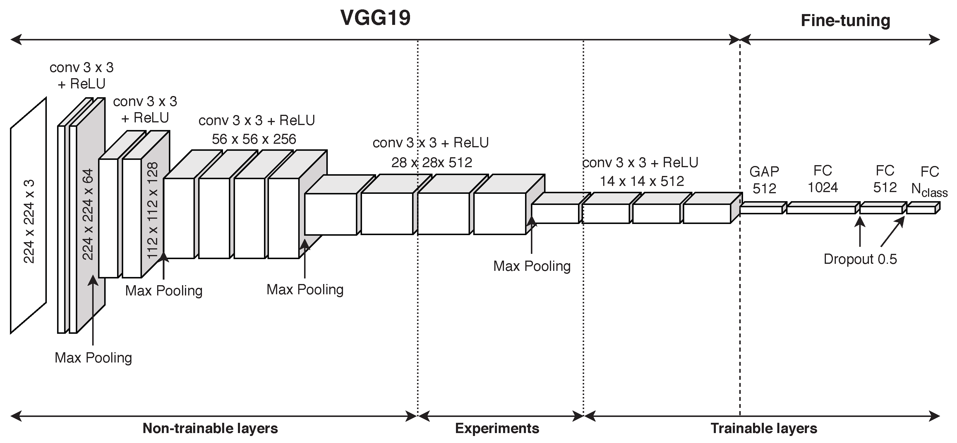
The first step of the fine-tuning process on VGG19 consists in the training of the network on the ImageNet competition dataset, though its evaluation classes have nothing in common with apparel, at first glance. Nevertheless, this first training provides the neural network with the ability to discriminate some basic features of images, which do not belong to any specific context, namely, lines, simple geometric shapes, and color stains. In this context, the term “features” refers to the mid-outputs of a CNN, obtained after the passage of the image in a single convolutional layer, and not to the list of seven features we described previously. Since, in this section, we approach only the logo detection, and the term “feature” is not ambiguous. The second step of fine-tuning consists of freezing the weights of a fixed number of initial layers of the network. The reason behind this choice is that simple features, such as edges, lines, and so on, are generally attributed to the very first layers of a neural network and they are useful in almost all image classifications and object detection tasks. Hence, a single training phase on the ImageNet dataset is sufficient to obtain acceptable weights for some of the first layers. The third phase, after having fixed the parameters of the first layers, is a second training on a barely different network topology. In this second training cycle, the last layer of the pre-trained VGG19 is removed and some fully-connected layers, loaded with random weights, are added in its place. As a matter of fact, the last layer of VGG19 is the one responsible for the classification itself, i.e., it outputs the ImageNet classes, which is certainly inappropriate for our scope. In detail, all convolutional layers of VGG19 are maintained, immediately followed by a Global Average Pooling (GAP), which reduces the size by taking only the average values of all the 512 output channels of the last convolution. Then, some experiments were made to detect the best Fully Connected (FC) layer dimension, and it comes out that a 1024 FC layer followed by a 512 FC layer is enough for our scopes (see Section 6). The last layer, as expected, is an FC one of size that equals the number of classes, 4 in the logo case (BOS, LINEAR, TREFOIL, and NONE). Between each FC layer, a Dropout layer of parameter is added. Those layers drop half connections, randomly, in order to prevent overfitting. The architecture of the network is illustrated in Figure 6. A batch size of eight images is used in the second training.
These added layers, together with the last ones of the base model, were the ones responsible to recognize more specific and elaborated features inside the input image, namely, logos themselves or part of them. The fact that layers increased the complexity of recognized features as the depth of the network increases was helpful in the development phase. As a matter of fact, this step allows us to extract some evaluation parameters for each layer, and to represent them by means of heatmaps, i.e., images that show which parts of the input image have been triggered at each layer. Figure 7 shows the heatmap obtained by the neuron activation values of the GAP layer, which is placed after the last convolutional layer of the network. The figure shows the original image, the overlap between the image and the heatmap, and the extracted heatmap.
Another technique that allows to work around the lack of images in a dataset, and that brings significant improvements in system accuracy at the same time, is the data-augmentation. Data-augmentation consists of applying some transformations to the training set images, before inputting them into the net. These transformations vary from rotations, stretches, zooms, splits, to channel shifts (in order to reach color variations). The benefit of using such a technique is that it provides the net with much more training information. Although it is a type of dummy information, it achieves the intended purpose. One last addition which leads to a slight increase in the overall accuracy percentage is the parameter called class-weight. The purpose of such a parameter is to apply an imbalance in the classification propensity of the net. Class-weight is applied because, by careful observation of the composition of Adidas AG™ datasets, it was discovered that clothes with the logo vastly outnumbered the ones without it. It is worth noting that assigning class-weights is a technique that may lead to biased results. For example, a accuracy on a validation dataset where logos are in a 9-to-10 ratio could mean that the network never outputs the no-logo class NONE, and this could happen if the logo class is heavily weighted during training. For this reason, confusion matrices and metrics such as precision and recall are also taken in account during experiments, checking the rate of false positives and false negatives. On the other hand, training a net on a highly imbalanced dataset is probably even worse, resulting in un-training the neural model on the less numerous classes. Thus, we choose to keep a balanced dataset, with about the same number of images for each class, but applying class-weights to take into account the fact that logos are very frequent in a real Adidas dataset. As a result, class-weight application has made the net more inclined to attributing a piece of apparel to a logo class (which can be one of the logo types, while MEDIUM or LARGE classes are inferred from which network has found the logo) than to the no-logo one (the class NONE).
4.2. Logo Detection through Standard Computer Vision Approaches
The method used for detecting small logos is a template matching method. This method was previously described by authors in [9], but it is reported here for clarity. The PCC [30] is used, with personalized kernels. Such personalized kernels are actually small images called templates. The approach of PCC has to be improved to search for such templates into the input images, instead of low-level kernels. The template of a logo is a grayscale image that represents the logo itself. One of the main problems is that logos in images are not always completely visible, or clear. Logos could be deformed by folds, or printed in a small corner of the garment. For these reasons, a plain image representing a logo is not sufficient for matching most of the logo occurrence in input images. Hence, templates are subject to rescaling, angular sliding, and rotations, prior to the PCC computation. In case of small logos, whose views can be easily occluded by other details in the apparel image, the left-hand side (LHS) and the right-hand side (RHS) of the logo are treated as two different templates. Each transformation of the template has to be matched with the input image. Such an approach has well-known limitations, which are outlined as follows:
- In input images, there is a wide variety of occlusions or deformations of the logo, e.g., rotations, angular sliding, and so on: this means that a large number of required transformations of the template;
- PCC is computed on each pixel of the input image, by sliding each template transformation on the whole image;
- false positive object detections are easy to obtain, since logos are composed mostly of geometric patterns, used also for other prints.
To approach the first two points, a downsampling is performed on the input image. The downsampling factor is specified later, when describing the algorithm. Then, the search area for computing the PCC is reduced to regions where logos are more likely to be found. There are also some drawbacks, e.g., if the downsampling reduces the image too much, some important information about the logo could be lost, and this could result in a decreasing of the method accuracy. Moreover, regions where a logo is expected to be found have to be chosen correctly to achieve good results using this algorithm. On the other hand, appropriate choices of the available regions and the sampling rate drastically reduce the computational time, leading to good results on the majority of the input images. As stated in the third point, false positives are easily obtainable, and they cannot be avoided using only the previously described downsampling and reduction. In our approach, we use a mask, which we apply to the given template. Such a mask puts weights, as a degree of importance, on each pixel of the template. In this specific application, a three-valued scale for masking a template is used, in order to differentiate three zones of the logo image: highly-relevant zones (which characterize well the logo—e.g., edges), common zones (which appear in each logo but also in other parts of the image—e.g., geometric patterns), and irrelevant zones (such as the background).
Precisely, the template is a grayscale image of the logo, which is usually much smaller than the input image. A mask is a three-valued grayscale image of the same size of the template. Let I be the two-dimensional matrix representing a grayscale version of the input image, and T the same for the template, and let n be the size of the template. M is a matrix of order n, representing a grayscale image used as a mask, whose values lie between 0 and 1. The punctual equation of PCC, applied to images, is as follows:
where j spans from to , and k from to , given and as the width and the height of the template T, respectively. is a portion of the image I with the same size of T and centered around . Scalars and are the average values of and T, respectively. (and, therefore, ) is the pixel value of that image at the coordinates computed from the center of that image. It is worth noting that the numerator is the covariance between I and T, and the denominator is the product of their standard deviations. Hence, the equation is invariant to affine transformations. This means that PCC is a robust method in case of varying light conditions, showing independence from several real-world lighting issues, since the main lighting contribution from objects is linear. Rearranging the Equation (1) allows us to gain a simplified equation that does not depend directly on the averages of the image and the template. This is useful to apply a mask M to the template, as follows:
where indexes are omitted for the sake of brevity. The value of PCC obtained in this way is still invariant to affine transformations.
The relevant region of the input image consists initially in the entire visible area of the garment in the image, obtained in the preprocessing phase: in fact, the binary image that represent the shape of the apparel product has value 0 on the background, and 1 otherwise. The initial template matching is performed on a downsampled grayscale version of the input image. The initial downsampling factor is 16. Equation (2) is computed for each pixel of coordinates in the search region, for each transformation of the template. It is worth noting that . Such a score has an immediate interpretation: a value close to 1 means a strong correlation between the portion of the input image and the template, whilst a value close to an inverse correlation. Since logos could have different backgrounds and colors, both correlation and inverse correlation denote a good match. In our approach, the PCC value is then transformed into a probability, between 0 and 1. A threshold is applied to find the most probable matching. Applying a threshold returns a set of regions, and these regions are used in the following step of the algorithm to perform the successive matching. Simultaneously, the downsampling on the input image is reduced to a factor of 8 in the second iteration and 4 in the third. Such an iterative process is repeated no more than three times in our system, in order to avoid high computational times. At the end of the iterative process, the remaining search regions become the regions where the logo was found, and a circle is drawn over it to indicate its position. Figure 8 shows the procedure for finding a small logo using PCC. Only the matching with the right-hand side of the logo is detailed, but the last image shows the results of both searches (LHS and RHS). In this case, the logo is clearly visible, but it could be confused with the background pattern: in fact, the first iteration of PCC in Figure 8c retrieves several false positives.
This approach is also applicable to other kinds of logos if other types of templates and masks are provided, giving very accurate results if appropriate template transformations are performed. Nevertheless, such a method is hardly generalizable to other datasets and an increasing number of iterations is required to generalize without losing accuracy, but predictably the computational cost of the algorithm increases too. A purely qualitative and visual analysis seems to confirm that the sum of all deep learning techniques and workarounds grants more appreciable results as the logo size increases, particularly with deformed or partially visible logos. On the other hand, it shows less sensitivity than PCC in detecting tonal logos (e.g., gray logos on a slightly lighter gray background)—those that are so tonal that they are barely recognizable even by human eyes. A more accurate evaluation of the results is presented in Section 6.
5. Other Features
Beside logos classification, methods for recognizing and classifying the other features are described in the following.
5.1. Stripes Recognition
Apart from logos, another notable feature to extract is the presence, location, and properties of the peculiar Adidas three-stripes. A description of brand relevant marks recognition is discussed in [9], where this approach was detailed first. The three-stripes detection needs specific geometric techniques, since their recognition is based on properties of parallelism and perpendicularity of strokes that compose the design. These properties, such as parallelism, perpendicularity, intersections between lines, could be evaluated by reasoning on the edges of the input image. Hence, the input image is transformed in a line image. The chosen methodology is the use of thinning algorithms and edge detection to perform this task.
The first step, whose goal is to obtain a rough approximation of the input image edges, is the computing of a gradient map. An opportune gradient map must be obtained, in order to preserve significant information about the clothing design. Clearly, colored realistic 3D-renderings or photographs do not have well-definite edges: instead, borders are recognized by discontinuity between a color and another. For this reason, a distance metric between two adjacent colors, which define different regions of the depicted clothing, should be defined. The first option would be to use the Euclidean distance of the RGB colors, but a better option consist of using a more accurate distance (such as [39]).
As expected, input images are mapped in the RGB color space. To perform the color distance, images must be mapped into the CIELAB color space, instead. Such a color space is also three-dimensional, and it is capable of denoting all visible color by a human eye. It consists of two channels and a lightness value. Two channels range from red color to green (A channel), and from yellow to blue (B channel). Thus, each pixel in an image is coded by using three parameters: L, A, and B. A peculiar metric, distance , is defined on CIELAB space by [39]. The distance is negligible between colors which are perceived as the same by our eyes, but it takes high values when these colors have “just noticeable differences”. Such a property grants that small color differences are measured precisely.
Using this distance, we compute the adjacent difference of each pixel to its neighbor on the left and its neighbor below, obtaining two different real valued images: and , respectively horizontal gradients and vertical gradients (defined for each pixel of the input image). Finally, with the formula , we compute the global gradient map, defined for each pixel (a first approximation of the input image borders). Thresholding this gradient map with an adaptive Gaussian threshold gives a binary output image representing the edges.
The obtained thresholded image is now a sort of sketch, a border image, which has to be thinned. After thinning, a pruning phase follows, to obtain all paths that compose the borders. Paths are useful to reason in geometric terms, and to match some specified patterns. In our case, the pattern to be retrieved consists of three parallel bands of the same width, i.e., six equidistant and parallel lines, in terms of paths. As for logos, the visibility of the three-stripes could be variable, and they are in the majority of cases partially hidden or deformed by the garment folds. Those visibility issues could affect their equidistance and parallelism properties. The three-stripes recognition is performed in two different steps. First, the image is segmented in order to obtain a set of significant regions where stripes are more likely to be found. Second, the algorithm performs the actual search in such significant regions, using the geometric properties of stripes.
Thanks to the preprocessing phase, a preliminary recognition of the type of the garment is performed. Then, relevant regions are extracted depending on such a type: in pants, stripes are searched on the side of the legs, while, for shirts and sweatshirts, the important regions correspond to sleeves. Finding relevant regions is of utmost importance in avoiding excessive computational times in the next step. The second step, in fact, analyze all paths in each relevant region. For each point of a path, the algorithm computes its neighborhood. The direction of the line is obtained by the orientation of its associate path. Knowing the direction, the algorithm goes across each point of the path, focusing only on points of the neighborhood that are perpendicular to the direction. A parallel path is recognized if and only if for each analyzed point in a certain range there is another point in the perpendicular direction and on the same side. Given a fixed distance, if a minimum of three and a maximum of seven parallel lines are detected in that range, the algorithm marks these lines as “three-stripes”. Such a heuristic is deliberately a rough estimate of the real geometric shape of the stripes, in order to prevent false negatives caused by occlusions, folds, deformations and so on.
5.2. Colors Segmentation
The color, or colors, of an article is another important feature to be extracted. It is a feature by itself, as explained in Section 3, but it is also used in determining the contrast between stripes and the background, and the composition of clothing prints and patterns. A brief overview of this approach was previously illustrated in [9]. Fashion industries develop new color names before each season, and the colors of articles are identified by such color names. As a result, the color palette of a product is composed according to that classification, which consists of thousands of color names, collected over the years. An appropriate mapping between each color name and its color code is required to correctly perform the segmentation. In order to provide data experts with meaningful statistical information from colors classification, defining a basic color palette of about 20 or 30 color names is advisable. Ref. [40] proposes another approach, which tries to learn the names of colors directly from the input images. In this work, we study a different solution, i.e., the creation of a small set of color names which are not related with those of Adidas, but that groups color shades and nuances in only 26 categories. This choice means a less accurate colors segmentation, but it has the advantage of being a more generalizable approach, and of preparing the dataset for successive statistical inferences.
As for stripes, an appropriate color space must be used, with its associated color distance. The color names are then mapped into that color space. A property of photograph or realistic renderings, as the images in Adidas dataset, is that their colors are not in solid blocks, but the regions that our eyes perceive as containing the same color are full of shades and nuances, which may invalidate the result of the segmentation algorithm. A distance that measures such shades as parts of the same color is then necessary. An appropriate choice, as discussed for three-stripes recognition, is the CIELAB color space, together with its color distance . The search of three most important colors in the article is performed in three phases. Region growing [41] is used in the first phase to perform an initial rough segmentation. Such a segmentation is operated on RGB input images. In order to measure the distance among these regions, a conversion transforms the input image into a LAB image. The distance is computed for regions two by two. For each region, the average color value is extracted, and the distance is measured between these values. Similar colors are thus grouped together, according to the CIELAB standard. The output of this second phase of the algorithm is a set of larger regions which better approximate the color area than the RGB regions. In the third and last phase, the distance between the average LAB value of each region and each color name code is computed. Hence, each region takes the name of the nearest color name. The algorithm returns the names of the three larger regions, and the percentage of covered area by such regions.
5.3. Deep Learning Based Feature Extraction
The extraction of prints, neck and sleeves’ shape is approached through deep learning techniques. In these cases, the availability of labeled images is sufficient to adopt this approach—although there are few in number, as in the logo case—and the separation among classes is clear enough. In particular, for prints and clothing patterns recognition, a fine-tuned VGG19 model is used, as for logo classification. Details are explained in Section 4.1.
During the training process, depending on which feature to detect, numerous adjustments are applied, varying from the number of FC layers that have been added to the starting VGG19 model, to the number of neurons for each of those, to the editing of datasets composition, or tuning parameters (e.g., the learning rate). Most of the work done regards the editing of the dataset composition. Together with Adidas data experts team, images were chosen from different seasons and collections, to achieve the best possible variety. This applies to all features (prints, neck, and sleeves). For example, heater pants and shirts have to be classified as not-printed (NORMAL) by the prints classifier, but most of the heater apparel images are pretty much the same, depicting gray solid clothes. To prevent the network to associate solid gray to heater type fabric, other non-solid or colored article images were required to Adidas team and added. Of course, data augmentation is also used, as for logo detection. As a matter of fact, the training dataset must be varied and consistent, and as less redundant as possible.
As previously outlined, not only dataset editing was used, but also variations on the number of FC layers and their sizes. For prints, after the GAP layer, four FC layers were added, with size 1024, 728, 512, and 2, respectively. For neck and sleeves, the 728 neurons layer was removed. The reasons for these adjustments is an empirical evaluation of the network accuracy after each experiment, which confirms that a first FC layer of 1024 neurons works better (as shown in the next section). The second FC layers of size 728 slightly increases accuracy of the prints classifier, and thus it is maintained since such a little improvement does not affect significantly the training time of the network. On the contrary, enhancement on neck and sleeves classification by this second FC layer are negligible.
Finally, the learning rate parameter was also tuned depending on the achieved accuracy. This parameter was set to a value of for all features. In Section 6, some accuracy tables are reported, containing examples of attempts that were done in order to reach the highest possible accuracy, implemented in the final modules.
6. Experimental Results
Modules of the above described system were tested separately, and experiments gain useful insights for improving the accuracy of each module. In addition, the detailed feedback that Adidas teams provide us were taken in account in the enhancement of the feature extraction system. In this section, some of the performed experiments on CNNs are reported, using the accuracy metric, to give a sense to the main decisions behind the deep learning approach we used. Then, the results of the standard computer vision modules are detailed, in terms of confusion matrices and accuracy metrics. The final accuracy values of all methods are highlighted in boldface font in the main text.
6.1. DL Modules
The very first experiment was the evaluation of a simple CNN architecture trained from scratch. The chosen architecture is a standard one where convolutional layers are followed by dense ones, as in a LeNet [42]. The dataset used for this first experiment is the one composed of 2616 images. The availability of a (manual) classification of those images allows us to divide the dataset in classes for logo detection. Only the type of logo was considered in this phase. In Table 1, accuracy results are reported, varying the number of dense and convolutional layers, as well as the learning rate. A dropout is applied at each training epoch, to prevent overfitting. The dataset was divided equally into a training and a test (or validation) sets, i.e., both sets contain the same number of images (1308). Accuracy is always measured on a validation set, consisting of different images from those in the training set. The table reported is related to the classification of type of logos. Similar results were obtained for other features.
Experiments with CNNs trained from scratch were intentionally left simple, since training a large deep network requires a huge amount of images and high computational time. Unfortunately, an accuracy value of about is not good enough for our scope.
The fine-tuning process brought significant improvements in accuracy percentage in comparison with deep learning approaches from scratch. The main reason behind this major enhancement is the use of the pre-trained network ability to recognize low-level features, reducing the impact of the lack of images in the dataset. In these subsequent experiments, the dataset is the same as in the previous case. There are 2616 images, half in the training set and half in the validation one, labeled with the logo types classification. Although the very first attempts were accomplished adopting a VGG16 network topology, it turned out that VGG19 was eventually a more efficient starting model. In Table 2 and Table 3, results of the fine-tuning with VGG16 and VGG19 architectures are shown, varying the number of frozen layers and the number of the fully-connected layers added at the end of the network. Moreover, the training time reduced substantially. All experiments were made on a Nvidia GTX 1070 GPU, and the average computational time per epoch is of s for logo types classifier, which was run for 80 epochs. Other classifiers based on VGG19 have similar execution time.
In Table 4, a further investigation on VGG19 fine-tuning was made, to choose the best value of the learning rate (i.e., the one that achieves better results in terms of accuracy, in an very low number of epochs).
An example result for the deep learning approach is shown in Table 5, for large logo types. The network recognize correctly of the images in a dataset of 86 unseen images, chosen by Adidas data experts (how the 86 number come out is explained later, in Section 6.2). Those images are unseen to the extent that are part of a new dataset provided by Adidas after the training phase. Thus, it does not contain any of the previous images in the 2616 dataset. The classification of these images is acceptable, with only a little misclassification of linear and original (BOS) logos. Table 5 shows the confusion matrix, with prediction classes on the first column and the reference on the first row. The number of images per class and their frequency percentages are also indicated. The inference of the class of an image takes usually 1–2 s of execution time, on a GTX 1070 GPU, for each feature to obtain by means of neural models. Thus, the expected average computational time for processing the whole validation dataset for large logo ranges from 86 s to 172 s. The exact computational times are unavailable, since in fact the validation tests were made by Adidas team on Adidas servers.
As another example, the very different problem of prints recognition is analyzed. The validation dataset contains 250 images, and the overall accuracy of the printed classifier is . The 250 images dataset is different from both the previous logo dataset (consisting of 86 images), and the manual classified dataset of 2616 images. The confusion matrix, as well as class frequencies are reported in Table 6. For computational times, the previous mentioned considerations hold.
Validation results from Adidas team for neck shape, sleeves, and material are not yet available. However, their models were trained using the datasets and the parameters specified in the following:
- Neck shape. A smaller dataset whose images were extracted from the 2616 images dataset is used. In detail, both test and training set consist of 630 images. All images were cropped in order to depict only the neck and a little portion of the article around the neck (examples are in Figure 3). A batch size of 2 is used for 80 epochs, and the learning rate had a value of . Data augmentation was used, as specified in the previous section. The final accuracy achieved is on the test dataset.
- Sleeves. As for neck shape, the dataset used for sleeves is a slightly smaller portion of the original one. It consists of 2400 images, of which 1550 belong to the training set, and 850 to the test set. A batch size of 2, and a training performed over 180 epochs with a learning rate of , grants the model an accuracy of on the validation dataset.
- Material. Since the material of an article is one of the most difficult feature to recognize even for a human observer, a larger dataset was required to Adidas data experts. Thus, they provide us with a dataset of 6300 images, which were then divided into a training set consisting of 2000 cotton, 2000 synthetic, and 200 viscose articles; and a test set consisting of 1000 cotton, 1000 synthetic, and 100 viscose articles. A batch size of 4 was used, and an 80 epochs training was performed with learning rate . The final accuracy achieved is .
The average times per epoch are of s for the neck shape classifier training; s for sleeves’ classifier training; and s for a material classifier. All processing times are evaluated on a PC with a GTX 1070 GPU.
Finally, a legitimate question would be the reason why a VGG19 should be used, stating that many other architectures are available, and some of these architectures are also better rated than VGG19 on surveys like [43]. An experiment on middle sized logos was made in order to determine the most appropriate network topology in our context. Results are shown in Table 7.
6.2. CV Modules
In logo detection, the type is not the only class to be predicted. The system searches first for large logos, and if nothing is found, the medium and the small logo searches are performed in the same cascade logic. The total execution time for logo detection depends on which logo is recognized first. If a large logo is detected, it takes only the inference time of the large logos neural model (i.e., 1–2 s). Otherwise, the time of inferring a medium logo is spent. The running time of the CV template matching algorithm, instead, is of about 30 s for each iteration. There are three Iterations for each template, i.e., for each type of logo to be detected. There are three logo types (see Section 3), but not all nine iterations are performed for each image, since the algorithm stops after finding one of them. Adidas data experts test this logic on a dataset of 290 images, and then they analyze separately the results of each classifier on logo types. In Table 8, predictions are compared to references in the confusion matrix, and the frequencies for each class is indicated.
The type of classification of the 86 over 95 images that depict large logos was shown in the previous section in Table 5. Performance of the template matching approach gains overall accuracy on small logos on the 200 images that were classified as REGULAR.The confusion matrix is shown in Table 9. It is worth noting that there are no small linear logos. In this particular dataset, there are none, but normally these logos are not recognized by our template matching algorithm. This is because a linear logo template must depict a sub-part of both BOS and trefoil logos (the “adidas” writing on the bottom of the logo, as shown in Figure 1), and this fact may generate a huge number of false positives.
Regarding the three-stripes module, results were obtained by comparing the output of the classification with a ground truth of 1375 images. Such a dataset contains also of images that does not belong to neither FULL LENGTH nor PARTIAL classes. The overall accuracy of stripes length is on that dataset.
Colors, instead, do not have a precise accuracy value, since both the color names and the coverage percentage are subjective attributes. On the contrary, the color module in combination with the prints and three-stripes classifiers gains measurable results. In the first case, the color module has to recognize the type of “composition”, choosing among SOLID, COLOR BLOCKS, and SMALL INSERT classes, as outlined in Section 3 and in Figure 5. On the 213 not-printed products recognized using the prints classifier, as in Table 6, the overall accuracy is . The confusion matrix and class frequencies are shown in Table 10.
The most frequent misclassification, in this case, regards solid color garments. The reason is the presence of small regions, such as logos, of a different color. Better results are achieved in the classification of tonal or contrasted stripes. As a matter of fact, the distance between the colors of the stripes and the background is used at this scope, and gains accuracy on the 1375 images dataset.
7. Conclusions and Future Works
In this work, main motivations, techniques and methods, and final results of a feature extraction software system were presented. The application domain is the fashion creative workflow of apparel industries, and in particular the visual analysis of the large amount of data obtained as outcomes of designer works, prior to the actual fabrication of the garment. The application was conceptualized and developed in synergy with Adidas AG™ data expert teams, who highlight main directions and most important features. The study had pointed out the diversity of features to be extracted, and the emerging of some challenging research problems. Above all, the lack of datasets and an insufficient literature on fashion domain led to the implementation of some state-of-the-art techniques in a personalized approach, until a robust and reliable system had been proposed. As a matter of fact, most of the presented techniques are well-known and extensively tested and described in literature, but the real challenge of this work is to choose wisely among the wide variety of existing solutions, since many of them are general techniques that are unreliable, unfeasible, or give poor results in the specific application domain of fashion. The novelty of this work resides mainly in the domain of application, although original methods were used in every system module. Extensive tests and experiments were performed both by authors and by Adidas teams. As a matter of fact, the system was refined at experimental time, showing finally good accuracy results in all its tasks. As future work, these results could be further enhanced, based on Adidas teams’ feedback. Moreover, an interesting future development could be the introduction of more cases/classes (e.g., other types of logos, or other types of clothes, such as bra or tank tops), thus refining the search to a wider variety of products. As another relevant future work, the proposed system could be applied to the social network domain, in order to detect logos, three-stripes, prints and other features in public images or photos posted by users. This information is useful for tasting the general sentiment of users about products with certain characteristics, discovering trends and tendencies, and thus promoting new articles.
References
Author Contributions
Conceptualization, L.D.; Data curation, L.D. and E.I.; Formal analysis, L.D. and E.I.; Funding acquisition, A.P.; Investigation, L.D., E.I. and G.M.; Methodology, L.D., E.I. and G.M.; Project administration, A.P.; Resources, A.P.; Software, L.D., E.I. and G.M.; Supervision, A.P.; Validation, L.D., E.I. and G.M.; Visualization, L.D., E.I. and G.M.; Writing—original draft, E.I.; Writing—review & editing, L.D., E.I., G.M. and A.P.
Funding
This research received no external funding
Acknowledgments
This work is funded by Adidas AG™. We are really thankful to Adidas for this opportunity.
Conflicts of Interest
The authors declare no conflict of interest.
References
- Jing, Y.; Liu, D.; Kislyuk, D.; Zhai, A.; Xu, J.; Donahue, J.; Tavel, S. Visual search at Pinterest. In Proceedings of the 21th ACM SIGKDD International Conference on Knowledge Discovery and Data Mining, Sydney, Australia, 10–13 August 2015; pp. 1889–1898. [Google Scholar]
- Pal, N.R.; Pal, S.K. A review on image segmentation techniques. Pattern Recognit. 1993, 26, 1277–1294. [Google Scholar] [CrossRef]
- Shi, J.; Malik, J. Normalized cuts and image segmentation. IEEE Trans. Pattern Anal. Mach. Intell. 2000, 22, 888–905. [Google Scholar]
- Smeulders, A.W.; Worring, M.; Santini, S.; Gupta, A.; Jain, R. Content-based image retrieval at the end of the early years. IEEE Trans. Pattern Anal. Mach. Intell. 2000, 22, 1349–1380. [Google Scholar] [CrossRef]
- Redmon, J.; Divvala, S.; Girshick, R.; Farhadi, A. You only look once: Unified, real-time object detection. In Proceedings of the 2016 IEEE Conference on Computer Vision and Pattern Recognition (CVPR 2016), Las Vegas, NV, USA, 26 June–1 July 2016; pp. 779–788. [Google Scholar]
- Dai, J.; Li, Y.; He, K.; Sun, J. R-FCN: Object detection via region-based fully convolutional networks. arXiv, 2016; arXiv:1605.06409. [Google Scholar]
- Szegedy, C.; Liu, W.; Jia, Y.; Sermanet, P.; Reed, S.; Anguelov, D.; Erhan, D.; Vanhoucke, V.; Rabinovich, A. Going deeper with convolutions. In Proceedings of the 28th IEEE Conference on Computer Vision and Pattern Recognition (CVPR 2015), Boston, MA, USA, 8–10 June 2015; pp. 1–9. [Google Scholar]
- Simonyan, K.; Zisserman, A. Very deep convolutional networks for large-scale image recognition. arXiv, 2014; arXiv:1409.1556. [Google Scholar]
- Donati, L.; Iotti, E.; Prati, A. Computer Vision for Supporting Fashion Creative Processes. In Recent Advances in Computer Vision; Springer: Berlin, Germany, 2019; pp. 1–31. [Google Scholar]
- Borji, A.; Cheng, M.M.; Jiang, H.; Li, J. Salient object detection: A survey. arXiv, 2014; arXiv:1411.5878. [Google Scholar]
- Viola, P.; Jones, M. Rapid object detection using a boosted cascade of simple features. In Proceedings of the 2001 IEEE Conference on Computer Vision and Pattern Recognition (CVPR 2001), Kauai, HI, USA, 8–14 December 2001; Volume 1, pp. I511–I518. [Google Scholar]
- Blaschke, T. Object based image analysis for remote sensing. ISPRS J. Photogramm. Remote Sens. 2010, 65, 2–16. [Google Scholar] [CrossRef]
- Geiger, A.; Lenz, P.; Urtasun, R. Are we ready for autonomous driving? The KITTI vision benchmark suite. In Proceedings of the 2012 IEEE Conference on Computer Vision and Pattern Recognition (CVPR 2012), Providence, RI, USA, 16–21 June 2012; pp. 3354–3361. [Google Scholar]
- Russakovsky, O.; Deng, J.; Su, H.; Krause, J.; Satheesh, S.; Ma, S.; Huang, Z.; Karpathy, A.; Khosla, A.; Bernstein, M.; et al. ImageNet Large Scale Visual Recognition Challenge. Int. J. Comput. Vis. 2015, 115, 211–252. [Google Scholar] [CrossRef]
- ImageNet Challenge Website. Available online: http://www.image-net.org/ (accessed on 28 March 2019).
- Viola, P.; Jones, M.J. Robust real-time face detection. Int. J. Comput. Vis. 2004, 57, 137–154. [Google Scholar] [CrossRef]
- Dalal, N.; Triggs, B. Histograms of oriented gradients for human detection. In Proceedings of the 2005 IEEE Conference on Computer Vision and Pattern Recognition (CVPR 2005), San Diego, CA, USA, 20–25 June 2005; Volume 1, pp. 886–893. [Google Scholar]
- Lowe, D.G. Object recognition from local scale-invariant features. In Proceedings of the 7th IEEE International Conference on Computer Vision (ICCV), Kerkyra, Greece, 20–27 September 1999; Volume 2, pp. 1150–1157. [Google Scholar]
- Bay, H.; Ess, A.; Tuytelaars, T.; Van Gool, L. Speeded-up robust features (SURF). Comput. Vis. Image Underst. 2008, 110, 346–359. [Google Scholar] [CrossRef]
- Girshick, R.; Donahue, J.; Darrell, T.; Malik, J. Rich feature hierarchies for accurate object detection and semantic segmentation. In Proceedings of the 27th IEEE Conference on Computer Vision and Pattern Recognition (CVPR 2014), Columbus, OH, USA, 24–27 June 2014; pp. 580–587. [Google Scholar]
- Girshick, R. Fast R-CNN. 2015. In Proceedings of the 2015 IEEE International Conference on Computer Vision (ICCV), Santiago, Chile, 13–16 December 2015; pp. 1440–1448. [Google Scholar]
- Redmon, J.; Farhadi, A. YOLO9000: Better, faster, stronger. In Proceedings of the 2017 IEEE Conference on Computer Vision and Pattern Recognition (CVPR 2017), Honolulu, HI, USA, 21–26 July 2017; pp. 6517–6525. [Google Scholar]
- Ren, S.; He, K.; Girshick, R.; Sun, J. Faster R-CNN: Towards real-time object detection with region proposal networks. arXiv, 2015; arXiv:1506.01497. [Google Scholar]
- Sermanet, P.; Eigen, D.; Zhang, X.; Mathieu, M.; Fergus, R.; LeCun, Y. Overfeat: Integrated recognition, localization and detection using convolutional networks. arXiv, 2013; arXiv:1312.6229. [Google Scholar]
- Liu, W.; Anguelov, D.; Erhan, D.; Szegedy, C.; Reed, S.; Fu, C.Y.; Berg, A.C. SSD: Single shot multibox detector. In Proceedings of the 14th the European Conference on Computer Vision (ECCV), Amsterdam, The Netherlands, 8–16 October 2016; pp. 21–37. [Google Scholar]
- Redmon, J.; Farhadi, A. YOLOv3: An Incremental Improvement. arXiv, 2018; arXiv:1804.02767. [Google Scholar]
- YOLO Website. Available online: https://pjreddie.com/darknet/yolo/ (accessed on 28 March 2019).
- Perez, L.; Wang, J. The Effectiveness of Data Augmentation in Image Classification using Deep Learning. arXiv, 2017; arXiv:1712.04621. [Google Scholar]
- Fashion-MNIST Dataset. Available online: https://github.com/zalandoresearch/fashion-mnist (accessed on 28 March 2019).
- Pearson, K. Note on regression and inheritance in the case of two parents. Proc. R. Soc. Lond. 1895, 58, 240–242. [Google Scholar]
- Suzuki, S.; Keiichi, A. Topological structural analysis of digitized binary images by border following. Comput. Vis. Graph. Image Process. 1985, 30, 32–46. [Google Scholar] [CrossRef]
- Gonzalez, R.C.; Woods, R.E. Digital Image Processing, 3rd ed.; Pearson Education: Upper Saddle River, NJ, USA, 2007. [Google Scholar]
- Saeed, K.; Tabedzki, M.; Rybnik, M.; Adamski, M. K3M: A universal algorithm for image skeletonization and a review of thinning techniques. Int. J. Appl. Math. Comput. Sci. 2010, 20, 317–335. [Google Scholar] [CrossRef]
- Chen, Y.S. The use of hidden deletable pixel detection to obtain bias-reduced skeletons in parallel thinning. In Proceedings of the 13th International Conference on Pattern Recognition, Vienna, Austria, 25–29 August 1996; Volume 2, pp. 91–95. [Google Scholar]
- Donati, L.; Cesano, S.; Prati, A. An Accurate System for Fashion Hand-Drawn Sketches Vectorization. In Proceedings of the 16th IEEE International Conference on Computer Vision Workshops (ICCVW), Venice, Italy, 22–29 October 2017. [Google Scholar]
- Chen, J.; Guennebaud, G.; Barla, P.; Granier, X. Non-Oriented MLS Gradient Fields; Computer Graphics Forum; Wiley Online Library: Hoboken, NJ, USA, 2013; Volume 32, pp. 98–109. [Google Scholar]
- FlickrLogos-32 Dataset. Available online: http://www.multimedia-computing.de/flickrlogos/ (accessed on 28 March 2019).
- Bianco, S.; Buzzelli, M.; Mazzini, D.; Schettini, R. Deep learning for logo recognition. Neurocomputing 2017, 245, 23–30. [Google Scholar] [CrossRef]
- Sharma, G.; Wu, W.; Dalal, E.N. The CIEDE2000 color-difference formula: Implementation notes, supplementary test data, and mathematical observations. Color Res. Appl. 2005, 30, 21–30. [Google Scholar] [CrossRef]
- Van De Weijer, J.; Schmid, C.; Verbeek, J.; Larlus, D. Learning color names for real-world applications. IEEE Trans. Image Process. 2009, 18, 1512–1523. [Google Scholar] [CrossRef] [PubMed]
- Adams, R.; Bischof, L. Seeded region growing. IEEE Trans. Pattern Anal. Mach. Intell. 1994, 16, 641–647. [Google Scholar] [CrossRef]
- LeCun, Y.; Bottou, L.; Bengio, Y.; Haffner, P. Gradient-based learning applied to document recognition. Proc. IEEE 1998, 86, 2278–2324. [Google Scholar] [CrossRef]
- Canziani, A.; Paszke, A.; Culurciello, E. An analysis of deep neural network models for practical applications. arXiv, 2017; arXiv:1605.07678. [Google Scholar]
Figure 1.
Types of Adidas logos.

Figure 2.
Prints and clothing patterns’ examples.

Figure 3.
Types of neck shapes.

Figure 4.
In “raglan” shirts, the junction between the body and the sleeves starts from the armpits and goes to the neck; the term “set-in”, instead, refers to those shirts that have the sleeves sewn with the body of the garment with a vertical closure.
Figure 4.
In “raglan” shirts, the junction between the body and the sleeves starts from the armpits and goes to the neck; the term “set-in”, instead, refers to those shirts that have the sleeves sewn with the body of the garment with a vertical closure.

Figure 5.
Detailed organization of system modules. Uppercase statements highlight inputs and outputs, while boxed ones emphasize the actual modules of the system. Solid arrows denote conceptual connections among modules, while dashed arrows denote inputs or outputs.
Figure 5.
Detailed organization of system modules. Uppercase statements highlight inputs and outputs, while boxed ones emphasize the actual modules of the system. Solid arrows denote conceptual connections among modules, while dashed arrows denote inputs or outputs.

Figure 6.
Network architecture used for logo detection. On top of the figure, which layers have been kept from the VGG19 architecture and which ones were added in the fine-tuning re-training phase are indicated. In such a second training, some layers are frozen, thus maintaining the ImageNet weights, and others are not. On bottom of the figure, frozen and trainable layers are specified. The decision of training or not some of these layers was made at experimental time (see Section 6).

Figure 7.
Heatmap of a nearly invisible medium logo.

Figure 8.
An example of logo detection using template matching.


Table 1.
Training of a simple Convolutional Neural Network (CNN) from scratch.
| # of Conv. Layers | # of Dense Layers | Learning Rate | Dropout | Accuracy |
|---|---|---|---|---|
| 4 | 3 | 0.001 | 0.5 | 0.731 |
| 4 | 4 | 0.001 | 0.5 | 0.733 |
| 5 | 4 | 0.01 | 0.5 | 0.742 |
| 5 | 5 | 0.01 | 0.5 | 0.738 |
Table 2.
Some tests on fine-tuning with VGG16 topology and relative accuracy values. The best choice of parameters in terms of validation accuracy is highlighted in boldface font.
Table 2.
Some tests on fine-tuning with VGG16 topology and relative accuracy values. The best choice of parameters in terms of validation accuracy is highlighted in boldface font.
| # of Added Layers | # of Frozen Layers | # of First Layer Neurons | Accuracy |
|---|---|---|---|
| 1 | 10 | 256 | 0.853 |
| 1 | 11 | 512 | 0.846 |
| 2 | 10 | 128 | 0.850 |
| 2 | 11 | 512 | 0.846 |
| 3 | 12 | 256 | 0.869 |
| 3 | 12 | 512 | 0.848 |
Table 3.
Some tests on fine-tuning with VGG19 topology and relative accuracy values. The best choice of parameters in terms of validation accuracy is highlighted in boldface font.
Table 3.
Some tests on fine-tuning with VGG19 topology and relative accuracy values. The best choice of parameters in terms of validation accuracy is highlighted in boldface font.
| # of Added Layers | # of Frozen Layers | # of First Layer Neurons | Accuracy |
|---|---|---|---|
| 2 | 11 | 256 | 0.889 |
| 2 | 12 | 512 | 0.890 |
| 3 | 12 | 512 | 0.893 |
| 3 | 13 | 1024 | 0.908 |
| 3 | 14 | 512 | 0.902 |
Table 4.
Learning rate parameter variations. The best choice of parameters in terms of validation accuracy is highlighted in boldface font.
Table 4.
Learning rate parameter variations. The best choice of parameters in terms of validation accuracy is highlighted in boldface font.
| Learning Rate | Accuracy | # of Epochs |
|---|---|---|
| 0.01 | 0.824 | 14 |
| 0.001 | 0.947 | 8 |
| 0.0001 | 0.68 | 19 |
Table 5.
Results on large logo detection on an unseen validation dataset, performed by Adidas team. The numbers of correct predictions per class (on the main diagonal of the matrix) are highlighted in boldface font.
Table 5.
Results on large logo detection on an unseen validation dataset, performed by Adidas team. The numbers of correct predictions per class (on the main diagonal of the matrix) are highlighted in boldface font.
| Prediction/Reference | BOS | TREFOIL | LINEAR | Frequency # | Frequency % |
|---|---|---|---|---|---|
| BOS | 0 | 0 | 46 | ||
| TREFOIL | 0 | 2 | 28 | ||
| LINEAR | 0 | 4 | 12 |
Table 6.
Results on prints classification on an unseen validation dataset, performed by Adidas team. The numbers of correct predictions per class (on the main diagonal of the matrix) are highlighted in boldface font.
Table 6.
Results on prints classification on an unseen validation dataset, performed by Adidas team. The numbers of correct predictions per class (on the main diagonal of the matrix) are highlighted in boldface font.
| Prediction/Reference | PRINTED | NORMAL | Frequency # | Frequency % |
|---|---|---|---|---|
| PRINTED | 7 | 220 | ||
| NORMAL | 7 | 30 |
Table 7.
Results on medium logo detection, using different architectures. The best choice of network and frozen layers in terms of validation accuracy is highlighted in boldface font.
Table 7.
Results on medium logo detection, using different architectures. The best choice of network and frozen layers in terms of validation accuracy is highlighted in boldface font.
| Network | # of Frozen Layers | Total # of Layers | Validation Accuracy |
|---|---|---|---|
| VGG19 | |||
| DenseNet | 369 | 714 | |
| InceptionV3 | 164 | 318 | |
| NASNetLarge | 401 | 776 | |
| ResNet50 | 94 | 182 |
Table 8.
Results on logo size detection on an unseen validation dataset, performed by the Adidas team. Overall accuracy is on 290 images. The numbers of correct predictions per class (on the main diagonal of the matrix) are highlighted in boldface font.
Table 8.
Results on logo size detection on an unseen validation dataset, performed by the Adidas team. Overall accuracy is on 290 images. The numbers of correct predictions per class (on the main diagonal of the matrix) are highlighted in boldface font.
| Prediction / Reference | REGULAR | MEDIUM | LARGE | Frequency # | Frequency % |
|---|---|---|---|---|---|
| REGULAR | 4 | 2 | 197 | ||
| MEDIUM | 0 | 0 | 9 | ||
| LARGE | 3 | 1 | 84 |
Table 9.
Results on small logo detection on an unseen validation dataset, performed by Adidas team. The numbers of correct predictions per class (on the main diagonal of the matrix) are highlighted in boldface font.
Table 9.
Results on small logo detection on an unseen validation dataset, performed by Adidas team. The numbers of correct predictions per class (on the main diagonal of the matrix) are highlighted in boldface font.
| Prediction/Reference | BOS | TREFOIL | Frequency # | Frequency % |
|---|---|---|---|---|
| BOS | 1 | 183 | ||
| TREFOIL | 15 | 17 |
Table 10.
Results on not-printed color combination on an unseen validation dataset, performed by the Adidas team. The numbers of correct predictions per class (on the main diagonal of the matrix) are highlighted in boldface font.
Table 10.
Results on not-printed color combination on an unseen validation dataset, performed by the Adidas team. The numbers of correct predictions per class (on the main diagonal of the matrix) are highlighted in boldface font.
| Prediction/Reference | SOLID | COLOR BLOCKS | SMALL INSERTS | Frequency # | Frequency % |
|---|---|---|---|---|---|
| SOLID | 0 | 0 | 166 | ||
| COLOR BLOCKS | 8 | 2 | 30 | ||
| SMALL INSERTS | 43 | 10 | 17 |
© 2019 by the authors. Licensee MDPI, Basel, Switzerland. This article is an open access article distributed under the terms and conditions of the Creative Commons Attribution (CC BY) license (http://creativecommons.org/licenses/by/4.0/).
Share and Cite
MDPI and ACS Style
Donati, L.; Iotti, E.; Mordonini, G.; Prati, A. Fashion Product Classification through Deep Learning and Computer Vision. Appl. Sci. 2019, 9, 1385. https://0-doi-org.brum.beds.ac.uk/10.3390/app9071385
AMA Style
Donati L, Iotti E, Mordonini G, Prati A. Fashion Product Classification through Deep Learning and Computer Vision. Applied Sciences. 2019; 9(7):1385. https://0-doi-org.brum.beds.ac.uk/10.3390/app9071385
Chicago/Turabian StyleDonati, Luca, Eleonora Iotti, Giulio Mordonini, and Andrea Prati. 2019. "Fashion Product Classification through Deep Learning and Computer Vision" Applied Sciences 9, no. 7: 1385. https://0-doi-org.brum.beds.ac.uk/10.3390/app9071385
Note that from the first issue of 2016, this journal uses article numbers instead of page numbers. See further details here.