Adaptive Compensation of Bandwidth Narrowing Effect for Coherent In-Phase Quadrature Transponder through Finite Impulse Response Filter

Abstract

Coherent in-phase quadrature (IQ) transponders are ubiquitous in the long-haul and the metro optical networks. During the transmission, the coherent signal experiences a bandwidth narrowing effect after passing through multiple reconfigurable optical add-drop multiplexers (ROADMs). The coherent signal also experiences a bandwidth narrowing effect when electrical or optical components of the coherent IQ transponder experience aging. A dynamic method to compensate the bandwidth narrowing effect is thus required. In the coherent optical receiver, signal bandwidth is estimated from the raw analog-to-digital converter (ADC) outputs. By adaptively adjusting the tap coefficients of the finite impulse response (FIR) filter, simple post-ADC FIR filters can increase the resiliency of the coherent signal to the bandwidth narrowing effect. The influence of chromatic dispersion, polarization mode dispersion, and polarization dependent loss are studied comprehensively. Furthermore, the bandwidth information of the transmitted analog signal is fed back to the coherent optical transmitter for signal optimization, and the transmitter-side FIR filter thus changes accordingly.

1. Introduction

Coherent line-cards using the polarization-division-multiplexed quadrature amplitude modulation (PDM-QAM) have been the de-facto standards for the metro and the long-haul optical fiber communications systems [1]. When a modulated signal passes through multiple reconfigurable optical add-drop multiplexers (ROADMs), the bandwidth of the propagating signal narrows down due to two effects. One is the spectral shape of the ROADM filter, and the other is the misalignment between the central frequency of the signal and the ROADM passband [2,3]. This inevitably leads to an increase in the observed bit error ratio (BER) at the receiving end and eventually causes the receiver to lose track of the signal. Moreover, the bandwidth narrowing effect due to the ROADM is relatively dynamic.

Several methods have been studied to quantify the effect of cascading ROADMs. In [4], an accurate model is developed to predict the final bandwidth of the signal after passing through multiple cascaded ROADMs. In [5,6], the weighted crosstalk method is used to estimate the transmission penalty, including the effects of signal bandwidth narrowing, crosstalk filtering, and nonlinear-enhance crosstalk. In [7], the impact of the random group delay ripple on multiple cascading ROADMs is thoroughly studied. In [8], one observes signal-to-noise ratio (SNR) for n times and determines the minimal SNR. Then, the probability of this minimal SNR being smaller than a specified target is evaluated through extreme value statistics. This approach improves the reliability to access the performance of cascaded ROADMs. In [9], the influence of the bandwidth narrowing effect on a probabilistically shaped 64-QAM system is evaluated using generalized mutual information (GMI). The shaping parameters can be optimized to improve the tolerance to the bandwidth narrowing effect.

With a comprehensive understanding from the theoretical models and experimental results above, different schemes to compensate the effects of the bandwidth narrowing have been demonstrated. In [10], digital pre-equalization is applied to the coherent transmitter based on the estimation of the signal’s bandwidth using an analytical model. The parameters in the analytical model are determined by the statistics from the measurement results. In [11], the maximum likelihood sequence estimation (MLSE) is used to mitigate inter-symbol interference (ISI) induced by the bandwidth narrowing effect. In [12], time-domain digital pre-equalization is used for a bandwidth-limited coherent communications system. The characteristics of the channel are generated from the coherent receiver through a digital adaptive equalizer. In [13], the bandwidth narrowing effect is studied in the context of elastic optical network. Different techniques, like bandwidth-variable transmitter and optical spectrum shaping, are used to compensate the bandwidth narrowing effect. In [14], the bandwidth-variable transceivers offer flexibility in adjusting both the symbol rate and the spectral efficiency. With the cascaded ROADMs, the balance between the optical filtering tolerance and the required SNR can be optimized. In [15], the data stream from the transmitter passes through a digital filter and generates the duobinary data pattern, which is more tolerant to the bandwidth narrowing effect.

In this work, we propose a novel scheme to compensate the bandwidth narrowing effect by simply using the finite impulse response (FIR) filters. First, we demonstrate that the bandwidth of the received signal can be estimated from the raw analog-to-digital converter (ADC) data samples. Then, we adaptively adjust the FIR filter in the coherent receiver to provide compensation according to the received signal bandwidth. The tolerance of the coherent receiver to the bandwidth narrowing effect is improved by 5 GHz, which is equivalent to the bandwidth degradation of the signal passing through >10 ROADMs [16]. Furthermore, the estimated signal bandwidth can be fed back to the coherent transmitter. By adaptively adjusting the FIR filter in the coherent transmitter, one can dynamically change the spectral shape of the coherent signal. The system tolerance to the bandwidth narrowing effect through the cascaded ROADMs is further improved. This scheme is relatively simple to implement, and it is also complementary to the other methods discussed above [10,11,12,13,14,15].

2. Experimental Setup and Signal Bandwidth Estimation

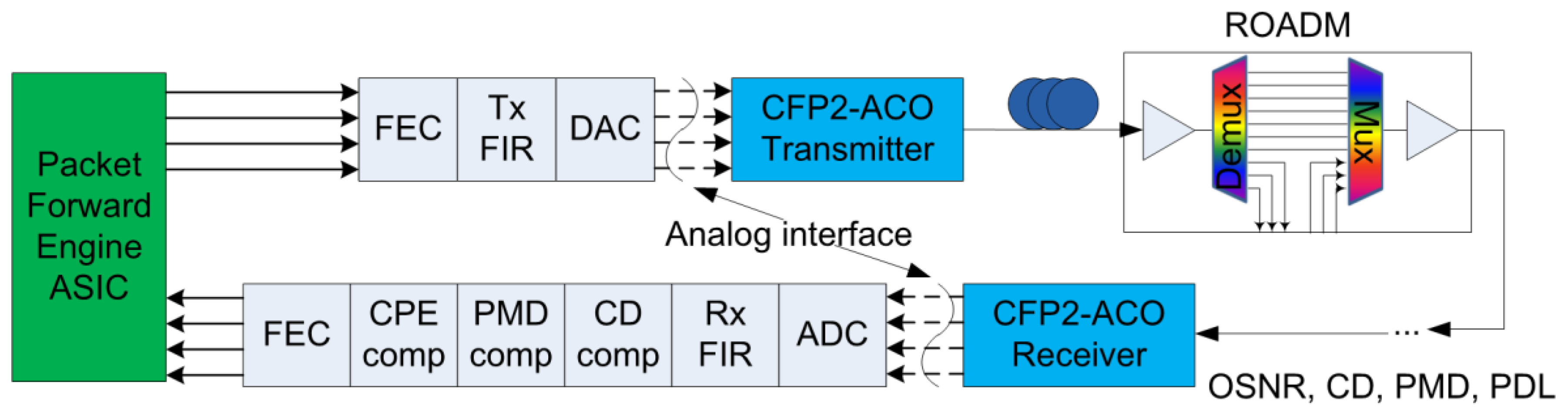
On top of the optical transport network, there is an Internet protocol (IP) network utilizing the packet forwarding engine (PFE) application-specific integrated circuit (ASIC) to forward the IP packets. It is very desirable to physically integrate the coherent transponder with the PFE, which will remove any client-side optical transponders to reduce the cost and power consumption. Figure 1 shows the architecture, which closely integrates the PFE, the digital signal processing (DSP) ASIC, and the coherent optical transponders. The client’s signal is received by the DSP and converted to the polarization-division-multiplexed quadrature phase shift keying (PDM-QPSK) modulation format at 30.1 giga-baud (GBd). The coherent optical transponder is a highly integrated C form factor two analog coherent optics (CFP2-ACO) module [17]. The payload of each transponder is either 100 gigabit Ethernet (GbE) or Optical Channel Transport Unit 4 (OTU4).

The IP traffic is converted into optical signal through the coherent transmitter and then transmitted through the long-haul optical communications system, which can have multiple cascading ROADMs. During the transmission, multiple optical impairments, such as chromatic dispersion (CD), polarization mode dispersion (PMD), and polarization dependent loss (PDL), can accumulate. At the receiver, the optical signal is coherently detected by beating with the local oscillator (LO). Then, the signal is converted back to the digital domain through the ADC. Most of the optical impairments are compensated by the DSP ASIC. Figure 1 depicts this detailed configuration. In addition, a network management layer oversees the whole long-haul system.

The digital analog converter (DAC), the circuit trace, the connector for pluggable optics, the radio-frequency (RF) amplifier, and the electro-optical modulator form the analog interface between the DSP chip and the coherent transmitter (Tx). Together with the ADC, the photodiode, the trans-impedance amplifier, the circuit trace, and the connector in the pluggable ACO form the analog interface between the coherent receiver (Rx) and the DSP chip. The received signal bandwidth is influenced by the bandwidth of both these analog interfaces. Although this influence is relatively static, it might degrade over the lifetime of the coherent transponder. Thus, a dynamic mechanism to compensate the bandwidth narrowing effect would also improve the tolerance to the component degradation.

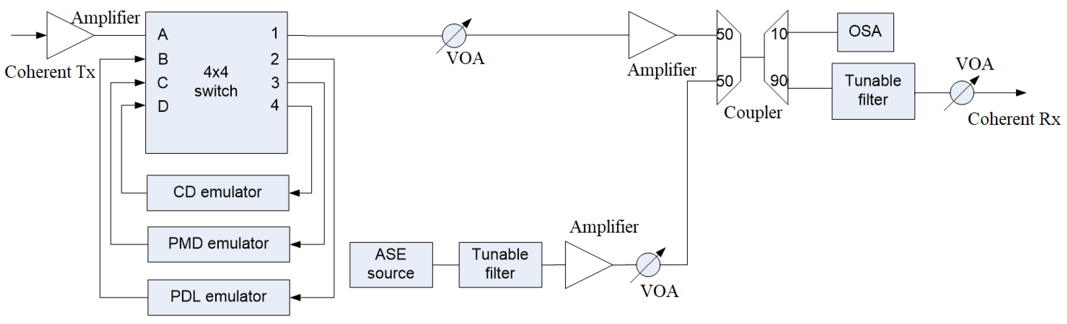
Figure 2 shows the experimental setup to study the bandwidth narrowing effect. CD, PMD, and PDL emulators are used to emulate various impairments in the transmission system. The 4 × 4 non-blocking optical switches can reconfigurably load either individual impairment or combined impairments. The noise produced by the amplified spontaneous emission (ASE) is added to adjust the optical signal-to-noise ratio (OSNR). An optical filter whose center frequency and pass-band are tunable is placed in front of the coherent receiver. The tunable filter is Finisar’s WaveShaper built on the liquid crystal on silicon (LCOS) technology. The filter’s passband closely resembles that of a wavelength selective switch (WSS), which is widely used in modern ROADM [4]. One noticeable difference is that with multiple cascading ROADMs, there is a steep roll-off at high-frequency content of the filter’s frequency response, which cannot be emulated by the WaveShaper. Despite this slight difference, one can adjust the pass-band of the tunable filter, allowing the emulation of the bandwidth narrowing effect to the coherent signal.

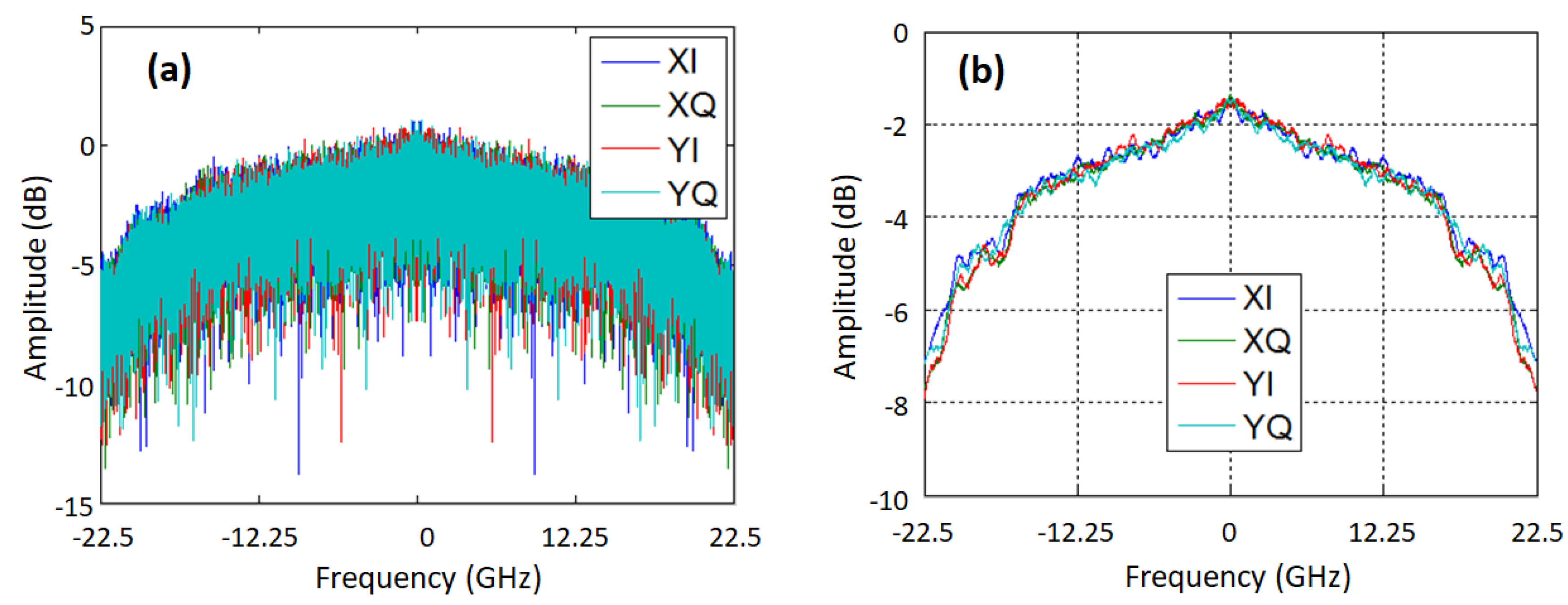
To achieve adaptive compensation of the bandwidth narrowing effect, we firstly estimate the signal’s bandwidth. The coherent DSP ASIC can provide a snapshot of the ADC raw data and store them in the random-access memory (RAM). The network management layer can extract the ADC raw data and perform fast Fourier transform (FFT) to calculate the spectrum of the modulated signal. The sample rate of the ADC is 45 GHz. There are 16,384 points for the ADC raw data, and FFT is then applied to the whole data set. The raw spectra from FFT are shown in Figure 3a. However, the data modulation makes it difficult to estimate the exact bandwidth. Thus, we apply the Savitzky-Golay filter [18] to smooth the raw spectrum. The length of the filter tap is 11, and the polynomial order of the filter is three. The Savitzky-Golay filter can improve the SNR with minimum distortion to the signal. It performs much better than the averaging filter, which filters out a significant portion of high frequency content of the signal. Figure 3b shows the spectrum after the Savitzky-Golay filter being applied.

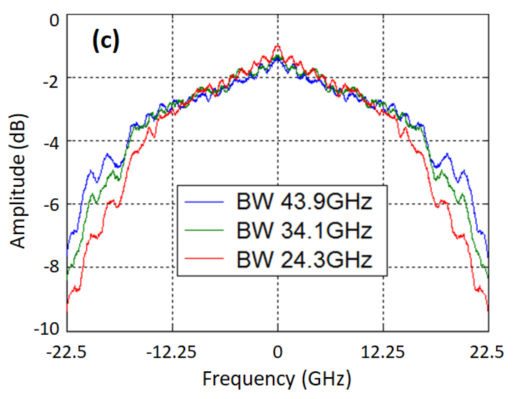
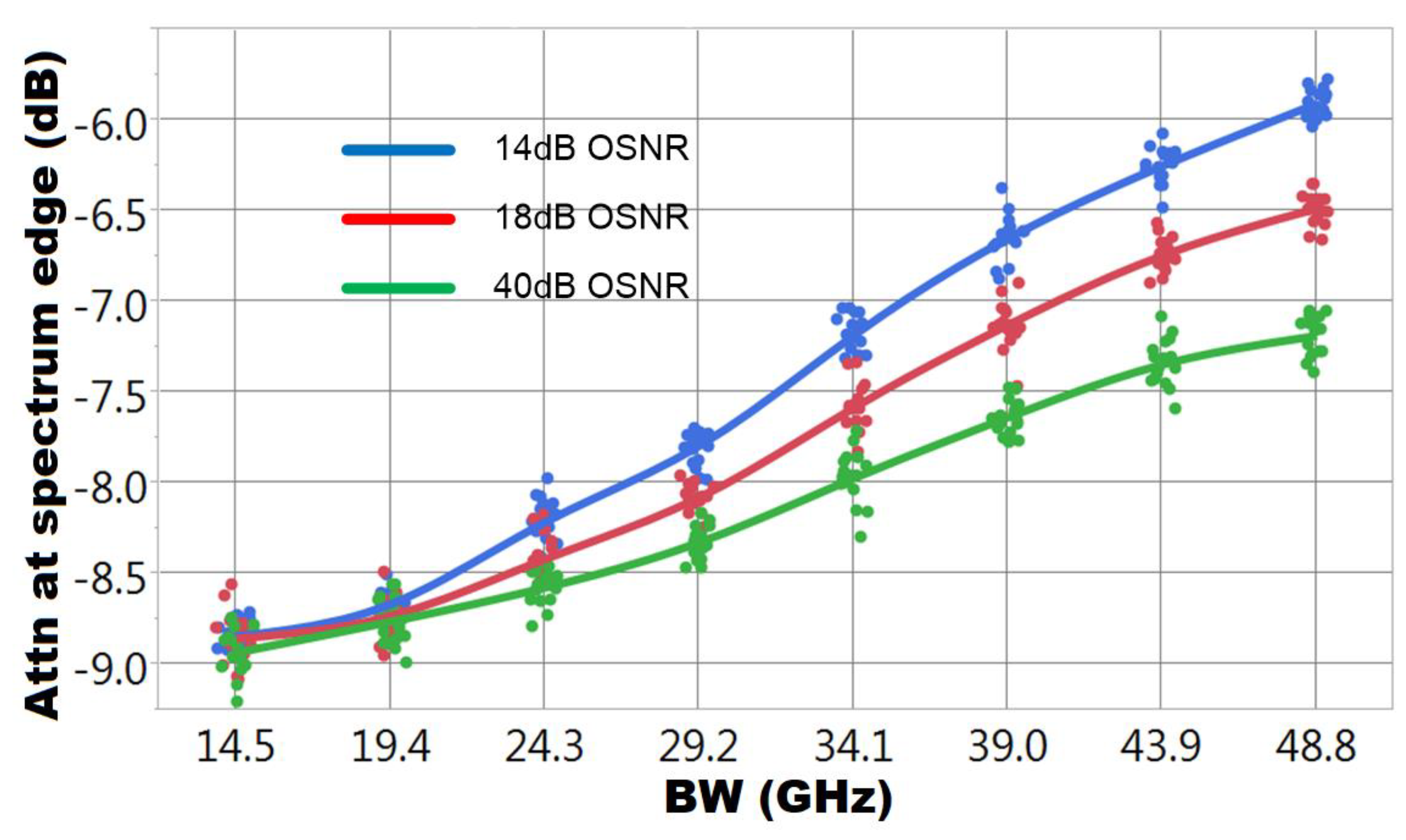
Next, we adjust the bandwidth of the optical tunable filter to emulate the narrowing effect for the coherent signal’s bandwidth. We define this parameter as the signal’s bandwidth. The spectra of the X-polarization in-phase tributary (XI) under different bandwidth are shown in Figure 3c. Clearly, the bandwidth narrowing effect is presented in the spectrum of the received signal. We defined the difference between the signal’s power at the spectrum’s edge (Nyquist frequency) and the one at the spectrum’s center as Attn_Edge. This parameter is closely related to the spectral shape of the signal and can be used to characterize the bandwidth of the signal. This value was further averaged over four tributaries to improve the accuracy. Figure 4 shows a roughly linear relationship between Attn_Edge and the signal’s bandwidth. There is small variation for Attn_Edge over different measurements, thus multiple measurements are used to improve the accuracy.

It is also noticeable that Attn_Edge is dependent on the SNR level. To estimate the signal’s bandwidth (BW) from Attn_Edge, one must approximately determine the SNR. In our experiment, the noise is emulated by an external ASE source. In such a condition, the SNR is approximately equivalent to the OSNR. One can thus use the pre-FEC BER to estimate the SNR [19].

In the long-haul optical communications system utilizing dense wavelength division multiplexing (DWDM), the noise is also coming from the nonlinear effect. In a modern DWDM system where coherent transponder is widely deployed, CD is continuously accumulated, and it is not compensated by the inline dispersion compensation module (DCM) anymore. Consequently, uncompensated CD broadens the spectrum of a coherent signal to a Gaussian-like shape. In the nonlinear regime where the per-channel power is larger than the optimal launching power, cross phase modulation (XPM) is the main source of fiber nonlinearity. However, most systems operate in the linear regime or weakly nonlinear regime where the per-channel power is smaller than the optimal launching power. Here, four wave mixing (FWM) is the main source of fiber nonlinearity. The noise generated from FWM approximately acts as the additive white Gaussian noise (AWGN) to the channel under consideration due to its Gaussian-like spectrum [20]. As a result, SNR is further reduced to a value smaller than OSNR. A well-known Gaussian noise (GN) model has been developed as a simple yet reliable tool to predict the performance of uncompensated coherent systems [21]. Thus, the pre-FEC BER can also be used to estimate SNR using the GN model.

Based on the discussion above, the measured Attn_Edge can be used to reversely estimate the signal’s bandwidth at the coherent receiver. In turn, the FIR filter in the receiver’s data path can be adaptive adjusted to compensate the bandwidth-narrowing effect based on the value of Attn_Edge.

3. Adaptive Compensation through Digital Filters

Simple FIR filters can be placed right after the ADC and before the frequency-domain CD compensation module. The typical usage of those simple FIR filters is to compensate the RF losses of the analog interface, and the tap values of the FIR filters usually remain unchanged during the lifetime of the coherent transponder. However, in this work, the tap coefficients of the FIR filters are dynamically optimized, particularly to compensate the bandwidth narrowing effect. As discussed in Section 2, the value of Attn_Edge is directly correlated to the signal’s bandwidth. One can use this value to see whether the signal’s bandwidth is limited. If so, one can adjust the simple FIR filter to provide more peaking to compensate the limited bandwidth.

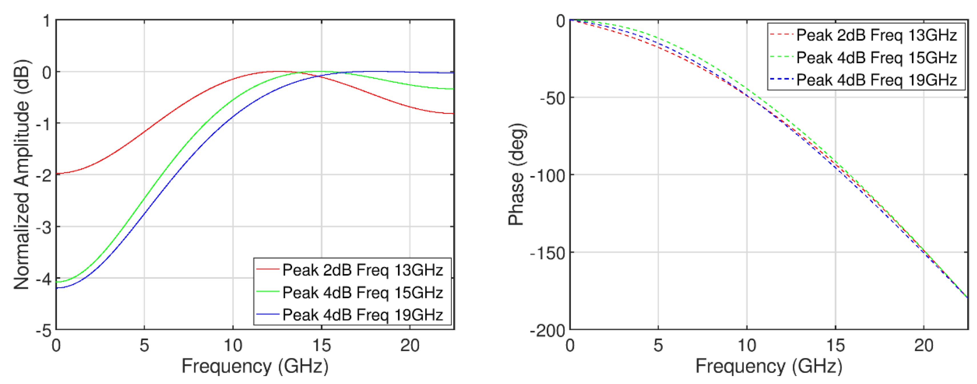
Two key parameters determine the shape of channel filters—peaking frequency and peaking amount. The peaking amount is the difference between the maximal frequency response and the frequency response close to the direct current (DC). The peaking frequency is where the maximal response locates in the frequency domain. The output of the FIR filter is a convolution between the input signal and the FIR’s impulse response, as shown in the equation below.

$$y(n)={\displaystyle \sum _{j=1}^{N}h\left(j\right)x\left(n-j\right)}$$

(1)

Here, x is the input signal to the FIR filter, h is the tap coefficient of the FIR filter, and N is the total number of taps. In the current DSP ASIC, N is equal to three. The FIR filter is T_s/2 spaced, where T_s is the symbol period. The tap coefficients of those digital filters are real numbers only. Also, four sets of the FIR filters (for four tributaries) share the same tap coefficients. These simplifications greatly reduce the complexity in the hardware implementation.

Next, we search different combinations of the tap coefficients and identify the desired spectral shapes. The desired range for the peaking frequency is from 13 GHz to 19 GHz, and the one for the peaking amount is from 1 dB to 5 dB. To obtain the target spectral shape, we first set the value of main tap to be one. Next, we perform a coarse scan on the values of precursor and postcursor. We adjust those values between −0.5 to 0.5 at the step of 0.1. By performing a Z-transform, the frequency response of FIR filter is determined. Then, we identify a small range of precursor and postcursor. Within this small range, the peaking amount and the peaking frequency are close to the target values. Furthermore, we optimize the values of precursor and postcursor by performing a fine scan within this small range. With only three taps, we sometimes cannot obtain both the desired peaking amount and the peaking frequency simultaneously. In those situations, we prioritize the peaking amount over the peaking frequency. Finally, we convert the representation of tap coefficients from floating-point number to signed-integer number. The conversion is based on the following rules—the tap coefficients are implemented by 8-bits registers with the most significant bit (MSB) being the sign bit; for the remaining seven bits, two bits are used to represent integer value, and five bits are used to represent fractional value. Figure 5 shows spectral shape dependence of a few FIR filters on the peaking frequency and the peaking amount. One advantage of those simple FIR filters is their approximately linear phase response, which minimizes the ripple in the frequency domain.

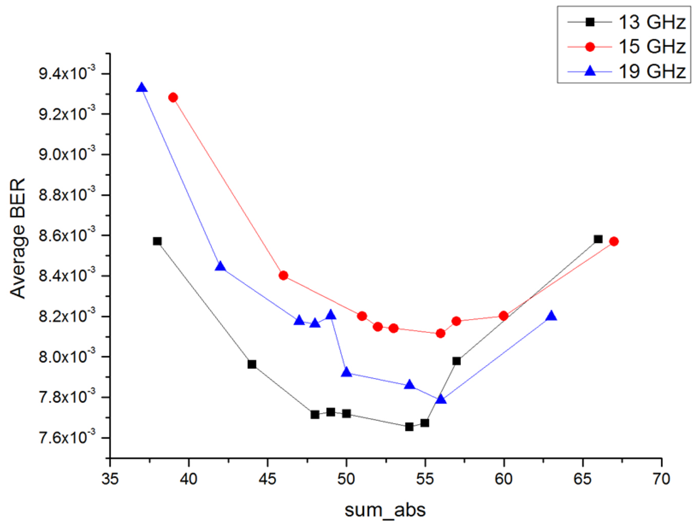
For each filter shape, there are multiple sets of tap coefficients satisfying the requirement. It is also important to consider the DC gain of the FIR filter, which is determined by the summation of the absolute value of those tap coefficients. A FIR filter with a high DC gain will lead the signal to being clipped, while a FIR filter with a low DC gain will lead the signal to being submerged under the noise. We optimize the DC gain of the FIR filter to achieve the best performance. We choose three typical filters: 2-dB peaking at 13 GHz, 4-dB peaking at 15 GHz, and 4-dB peaking at 19 GHz, corresponding to the three filters shown in Figure 5. We adjust the DC gain of the FIR filter while maintaining the spectral shape in the frequency domain. We measure the BER under different DC gain and summarize the results in Figure 6. As seen, for each filter’s shape, there is an optimal DC gain setting leading to minimum BER. In the following sections, we set the DC gain of the FIR filter to the optimal point.

In general, the spectral response of the FIR filter should be inverse to the overall frequency response of the cascaded ROADMs for equalization. When a signal has a relatively high bandwidth with a small number of cascading ROADMs, the optimal filter has a small peaking amplitude and a small peaking frequency. Otherwise, more noise will be amplified. When a signal has a low bandwidth due to larger number of cascading ROADMs, the optimal filter should have a large peaking amplitude and a large peaking frequency. In this way, any reduction of the signal’s bandwidth will be compensated by this adaptive FIR filter.

We first study the scenario where no FIR filter is applied. However, we obtain a subpar BER result. The performance degradation is much more severe when various impairments are included. The reason is that the optical and the electrical components in the receiver’s data path accumulate the limitation on the received signal’s bandwidth. Even when the receiver’s signal bandwidth is not limited by the filter-narrowing effect due to the cascading ROADMs, a FIR filter with certain peaking amount is still needed to compensate the bandwidth limitation introduced by various components in the receiver’s data path, as discussed in the introduction. We experimentally identify that a mild FIR filter with 2-dB peaking at 13 GHz provides the optimal results across different scenarios. The performance is similar to that reported in [22], where a coherent transponder is built with discrete premium components. This demonstrates that the mild FIR compensates the bandwidth limitation of integrated coherent receiver.

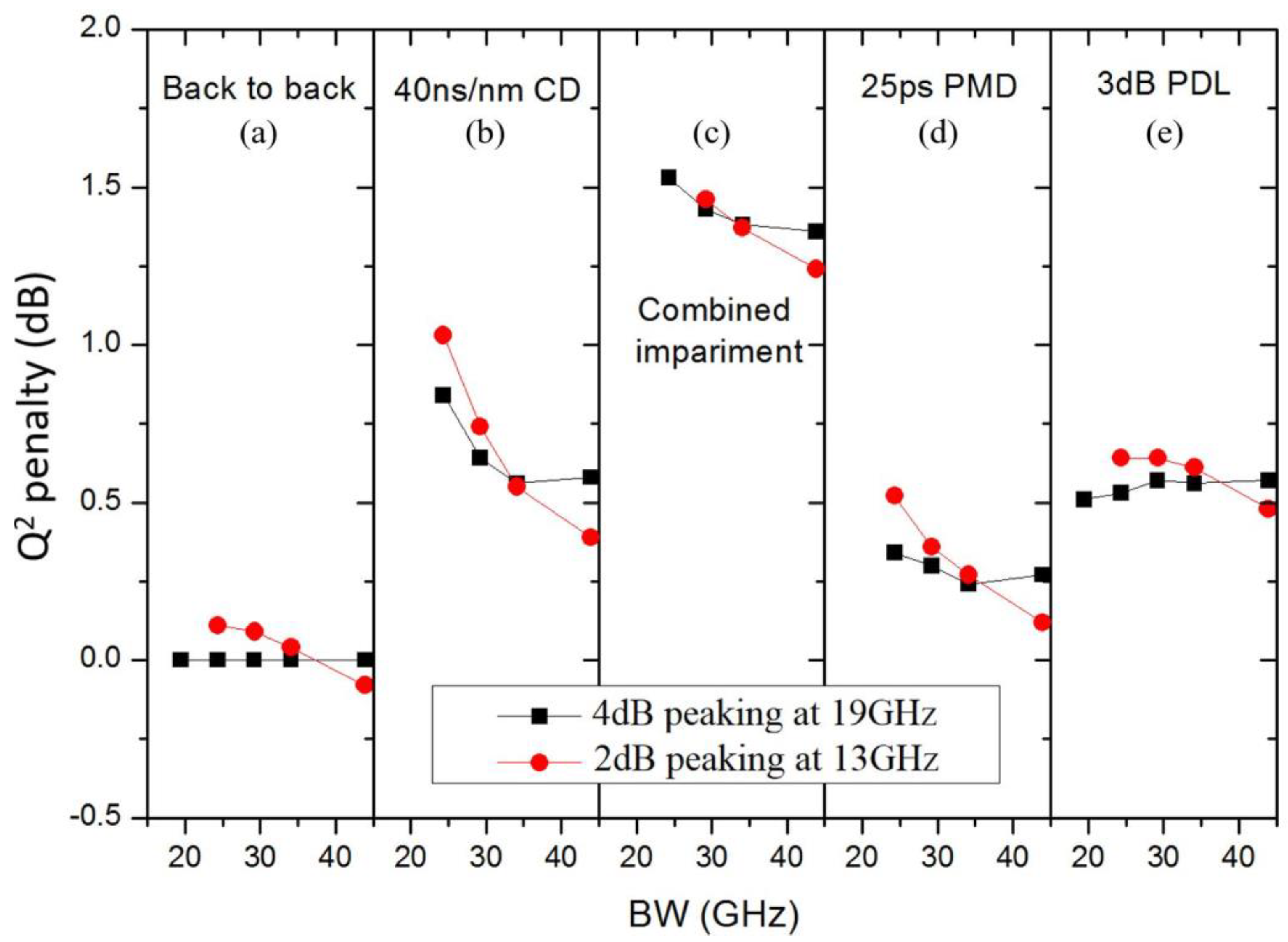
To demonstrate the advantage of our proposed method, we also select a strong FIR filter with 4-dB peaking at 19 GHz for further study. It is expected that the mild FIR filter will perform better when the signal’s bandwidth is large, while the strong FIR filter will perform better when the signal’s bandwidth is small. Through the experimental measurements under different transmission impairments, we validate this prediction. The results are summarized in Figure 7.

For these two settings, we measure the pre-FEC BER at 16-dB OSNR with a receiver optical power of −18 dBm. This is close to our system’s end-of-life specification, which is the summation of the required OSNR for the coherent receiver and the reserved margin for operation. The pre-FEC BER is reported by the DSP ASIC using the output of the FEC decoder. Furthermore, one can use the pre-FEC BER to estimate the SNR. We first convert the measured BER to the Q² factor. Next, we choose the baseline as the measured Q² factor in the back-to-back scenario with the strong FIR setting. We determine the penalty by calculating the difference between the Q² factor under the specific scenario and the Q² factor of the baseline scenario.

In the subplot of the back-to-back scenario, the penalty of the Q² factor under the strong FIR setting is always zero, since this is chosen as the baseline. With the signal’s bandwidth larger than 40 GHz, we obtain a negative penalty for the mild setting, which indicates a better BER performance. However, when the signal’s bandwidth is smaller than 30 GHz, we obtain a positive penalty for the mild setting, which indicates a worse BER performance. In the other scenarios, the penalty in the Q² factor is always positive due to the fact that the transmission impairments such as CD, PMD, and PDL cause the degradation in the BER. Still, we can notice that the mild FIR setting performs better with the signal’s bandwidth larger than 40 GHz, while the strong FIR setting performs better with the signal’s bandwidth smaller than 30 GHz. Those experimental results agree with the analysis above. In the scenarios of back-to-back, 3-dB PDL, and combined impairment, as shown in Figure 7a–c, a coherent receiver using a strong FIR setting can still recover the signal with 20-GHz signal’s bandwidth; however, a coherent receiver using the mild FIR setting fails to recover this signal. This indicates that the operation range of the coherent receiver using 4-dB peaking at 19 GHz (strong FIR setting) is 5 GHz larger than that of the coherent receiver using 2-dB peaking at 13 GHz (mild FIR setting). A 5-GHz improvement on the tolerance to the bandwidth narrowing effect will allow the coherent signal to pass 10 additional ROADMs [16].

In the data path of the coherent receiver, there is another adaptive equalizer (AEQ) to track the state of polarization (SoP), de-multiplex the orthogonal polarizations, and compensate the PMD. It is illustrated as the “PMD Comp” block in Figure 1. The AEQ also has multiple taps, thus a large amount of PMD can be compensated. To some degree, the bandwidth-narrowing effect can be partially compensated by this AEQ. The advantages of AEQ are high loop bandwidth and small response time. Thus, the equalizer can quickly track and dynamically compensate the bandwidth narrowing effect. However, there are certain limitations associated with the AEQ. The first limitation from AEQ is its complexity. The AEQ is a 2 × 2 equalizer with tap coefficients being complex numbers. It has large power consumption and long latency as well. The second limitation is that AEQ is placed after the CD compensation block. Thus, the bandwidth narrowing effect will increase the noise floor of the CD compensation block. The third limitation is that the quality of the signal impacts whether AEQ converges. When the bandwidth of the signal is severely narrowed down to <20 GHz, we notice that the coherent receiver cannot lock due to the fact that the AEQ cannot converge anymore. This can be seen from Figure 7a,c,e, where there are no data points for the mild FIR setting. When we apply the strong FIR setting to partially compensate the bandwidth narrowing effect, the AEQ converges, and the coherent receiver locks. We summarize the difference between two types of equalizers in

Table 1. Comparison between Rx FIR filter and PMD adaptive equalizer.

Parameters	Rx FIR Filter	PMD AEQ (Adaptive Equalizer)
Main function	Static loss compensation for RF channel	SoP tracking and PMD compensation
Location	Before CD block	After CD block
Tap coefficients	Real value	Complex value
Power consumption	Small	Large
Complexity	Simple tap-and-delay	Complicate 2 × 2 butterfly
Feedback mechanism	Spectrum from ADC raw data	Blind equalization or data-aided equalization
Loop bandwidth	Low	High
Number of taps	Small	Moderate
Impact of signal’s bandwidth	Minimal	AEQ may not converge with small bandwidth

.

The influence of these two types of equalizers on the optical performance of the coherent transponder can also be viewed in the experimental results above. For example, in Figure 7d, where the impairment of 25-ps PMD is presented, we notice that the penalty in Q² factor for the mild FIR setting is increased from 0.1 dB to 0.5 dB when the signal’s bandwidth is reduced from 50 GHz to 20 GHz. This shows that, even though the AEQ for PMD compensation can adjust its spectral response, the impairment due to the signal’s bandwidth narrowing effect cannot be fully mitigated by the AEQ alone. By changing the simple Rx FIR filter from the mild setting (2-dB peaking at 13 GHz) to the strong setting (4-dB peaking at 19 GHz), the penalty in Q² factor is reduced from 0.5 dB to 0.3 dB with 20 GHz signal’s bandwidth, demonstrating the performance improvement from the simple Rx FIR filter on top of the AEQ. Similarly, this performance improvement can also be observed when other types of optical impairments are introduced, as shown in Figure 7. Overall, both the AEQ for PMD compensation and the Rx FIR for channel loss compensation can be simultaneously used to improve the tolerance to the bandwidth narrowing effect of the coherent signal passing through multiple cascading ROADMs. A complementary method is to use the PMD equalizer to compensate the dynamic change of the signal’s bandwidth and use the simple FIR filter to compensate the slow drift of the signal’s bandwidth.

In addition to post-compensation at the Rx side, it is beneficial to apply pre-compensation on the Tx side as well. The Tx FIR is located after the FEC layer and before the DAC input. Most applications use those FIR filters to compensate the relatively static loss of the RF channel between the DAC’s output and the Mach-Zehnder modulator (MZM) in a set-and-forget approach. Since we can estimate the BW of the signal, we can also adaptively adjust the Tx FIR to pre-compensate the narrowing effect of signal’s bandwidth. In addition, the Nyquist filter is widely used to improve the spectral efficiency, which is usually a raised cosine (RC) filter or a root raised cosine (RRC) filter. The roll-off factor for the RC filter or the RRC filter determines the spectral response [23]. Thus, the key parameters of the FIR in the coherent transmitter are the peaking amplitude, the peaking frequency, and the roll-off factor. To determine the tap coefficients, the frequency response of the FIR filter with the desired peaking frequency and the peaking amount is first multiplied with the frequency response of the Nyquist filter. Next, a reverse Z-transform is performed to solve the coefficients of the combined filter.

As a demonstration, we apply the peaking filter and the Nyquist filter together to the Tx FIR. The number of taps in the Tx FIR is 17, and the FIR filter is T_s/2 spaced. We use the RRC filter with the roll-off factor of one as the Nyquist filter. We adjust the peaking amount from 1 dB to 9 dB while keeping the peaking frequency at the Nyquist frequency. We measure the optical spectra using a high-resolution optical spectrum analyzer (Finisar Wave Analyzer 1500) and summarize the results in Figure 8. As seen, the optical spectra clearly show the influence of different peaking values, demonstrating the feasibility of using Tx FIR to pre-compensate the bandwidth narrowing effect.

The capability of the FIR filter to adjust the signal’s spectrum is limited by the total number of taps. Usually, the FIR filters in the Tx have many taps and are independently controlled for each tributary. Thus, the Tx FIR allows great capability and flexibility for pre-compensation of the bandwidth narrowing effect. In general, with the bandwidth narrowing effect, one should increase the peaking amplitude, increase the peaking frequency, and reduce the roll-off factor. These parameters can be adjusted independently or simultaneously.

We summarize the experimental parameters in

Table 2. Experimental parameters for the Rx FIR filter and the Tx FIR filter.

Parameters	Value and Range
Receiver Optical Power (dBm)	−18
Transmitter Optical Power (dBm)	1
Optical Signal to Noise Ratio (dB)	16
Baud Rate (GBd)	30.1
Chromatic Dispersion (ns/nm)	40
Polarization Mode Dispersion (ps)	25
Polarization Dependent Loss (dB)	3
Signal Bandwidth (GHz)	20 to 50
Rx FIR Peaking Frequency (GHz)	13 to 19
Rx FIR Peaking Amount (dB)	1 to 5
Tx FIR Peaking Amount (dB)	1 to 9

below for both the Tx FIR filter and the Rx FIR filter.

4. Application Scenarios for Different Network Topologies

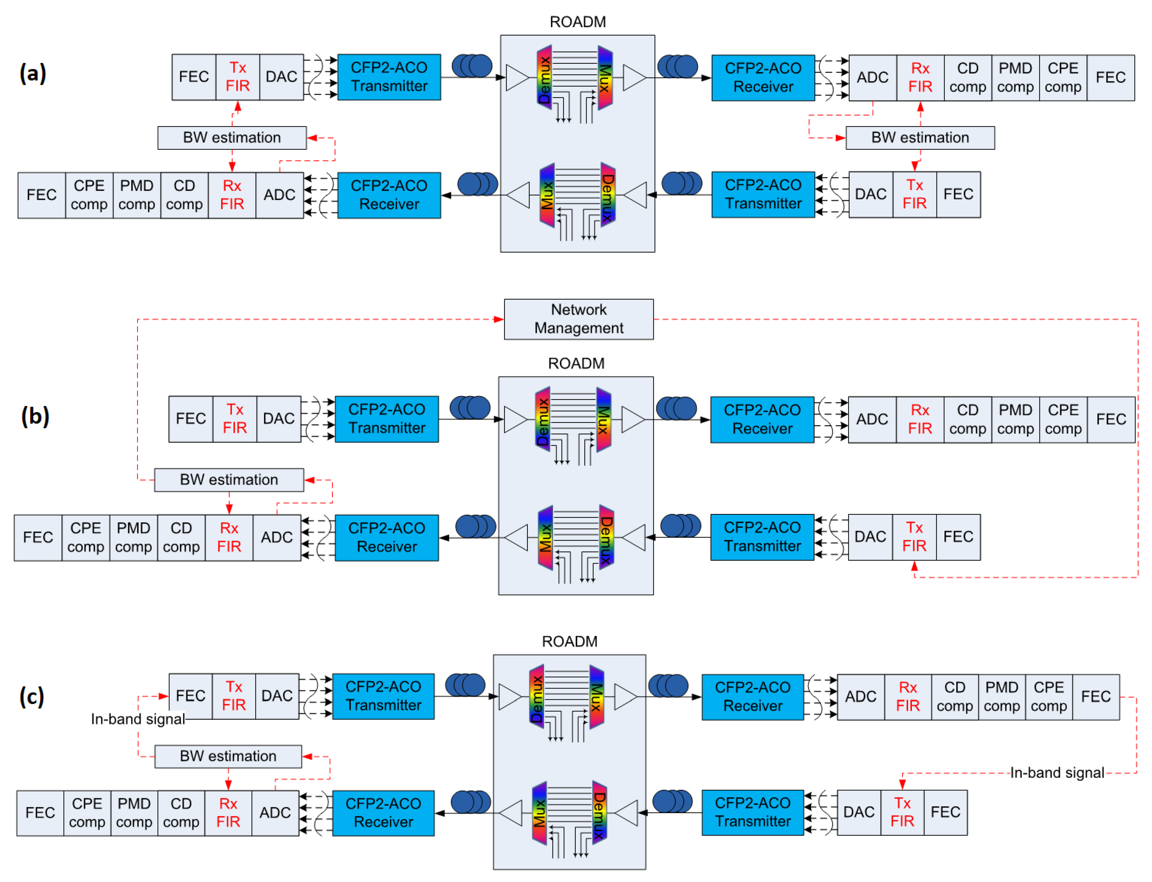
Different application scenarios exist with various network topologies. For each network topology, there is a different approach to apply the demonstrated method, as depicted in Figure 9. For most of the scenarios in the network, there are bi-directional links. Here, the transmitter of the network node one on the east end goes to the receiver network node two on the west end, while the transmitter of the network node two on the west end goes to the receiver of the network node one on the east end. The links in both directions go through the same number of ROADMs. The ROADMs in both directions are usually of the same type, from the same vendor, and under the same ambient environment. Thus, we can assume that the bandwidth narrowing effect in the east–west direction is the same as that in the west–east direction. In this case, one can estimate the bandwidth from the Rx of node 2 on the west end and use this information to adjust the FIR filter on the Tx of node 2. Hence, the characteristics of the west–east link are improved. This approach is shown in Figure 9a.

Furthermore, one can also send the estimated information of the signal’s bandwidth to the network management layer. The network layer will relay the information to the other end of the link accordingly. This approach is shown in Figure 9b. In addition, another approach is to send the information of the bandwidth in the reverse direction through the in-band signal, which can be embedded in Internet protocol (IP) packet or optical transport network (OTN) frame. This approach is shown in Figure 9c. Once the information is received by the other end, the FIR filter on the Tx side can be configured accordingly. For example, the Rx side of node two estimates the signal bandwidth in the east–west direction. This information is sent through the Tx of node two to the Rx of node one in the west–east direction through two approaches above. Once the node one receives the bandwidth information, it can adaptively adjust its Tx FIR for the pre-compensation that improves the performance of the east–west link. These two approaches can extend the application to any network scenario, although it will take longer time to adjust the Tx FIR to the appropriate setting.

A typical process is depicted below. Initially the FIR filters at both the Rx and the Tx sides are loaded with the default tap coefficients to compensate the channel loss of the analog interfaces. Next, the bandwidth of the received signal is estimated, and the Rx FIR is adaptively adjusted. Since one can calibrate the optical spectrum of the Tx signal and estimate the electrical spectrum of the Rx signal based on the raw data from the ADC, one can derive the degradation due to multiple cascading ROADMs. This information can be then fed back to the Tx directly in the bi-directional case or through the in-band signal/network management layer in the other case. Then, one can adjust the Tx FIR filter in one step based on a certain pre-calibrated table. Next, the Rx FIR filter can be adaptively adjusted to compensate any dynamic bandwidth narrowing effect.

The adaptive nature of the demonstrated method is well suited for real deployment. In the case with cascaded ROADMs, the spectral response of multiple filters will vary inadvertently. By estimating the spectrum of the received signal from the raw data of the ADC samples, one can dynamically adjust the simple FIR filter, which is implemented after the ADC, to compensate the bandwidth narrowing effect. This leads to an improved performance for the long-haul optical communications system.

5. Conclusions

Both the pre-compensation from the transmitter’s FIR filter and the post-compensation from the receiver’s FIR filter are demonstrated to compensate the bandwidth narrowing effect. The bandwidth of the received coherent signal is estimated from the raw output of the ADC with the improved accuracy by using Savitzky-Golay digital filter. No coherent receiver locking or data recovery is needed. The adaptive equalization of the FIR filter can improve the system’s tolerance to the bandwidth narrowing effect. This process can be done in real time with running traffic. The proposed method is critical for the coherent signal with high baud rate and high spectral efficiency, such as a single-carrier 64-GBd 16-QAM signal running with 400-Gb/s information bits.

6. Patents

A US patent was granted for the work presented in this paper.