Regularized Urdu Speech Recognition with Semi-Supervised Deep Learning

Abstract

Automatic Speech Recognition, (ASR) has achieved the best results for English, with end-to-end neural network based supervised models. These supervised models need huge amounts of labeled speech data for good generalization, which can be quite a challenge to obtain for low-resource languages like Urdu. Most models proposed for Urdu ASR are based on Hidden Markov Models (HMMs). This paper proposes an end-to-end neural network model, for Urdu ASR, regularized with dropout, ensemble averaging and Maxout units. Dropout and ensembles are averaging techniques over multiple neural network models while Maxout are units in a neural network which adapt their activation functions. Due to limited labeled data, Semi Supervised Learning (SSL) techniques are also incorporated to improve model generalization. Speech features are transformed into a lower dimensional manifold using an unsupervised dimensionality-reduction technique called Locally Linear Embedding (LLE). Transformed data along with higher dimensional features is used to train neural networks. The proposed model also utilizes label propagation-based self-training of initially trained models and achieves a Word Error Rate (WER) of 4% less than that reported as the benchmark on the same Urdu corpus using HMM. The decrease in WER after incorporating SSL is more significant with an increased validation data size.

1. Introduction

Automatic Speech Recognition (ASR) can be a vital component in artificially-intelligent interactive systems. After more than 50 years of research, ASR is still not a completely solved problem. ASR consists of three main components. These are, (a) extraction of useful features from speech for recognition of language phonemes or words, (b) classification of extracted features into words and (c) probabilistic modeling of predicted words based on language grammar and dictionary. The most famous features used for ASR are the Mel Frequency Cepstral Coefficients (MFCC). MFCC are found by taking the Discrete Cosine Transform (DCT) of logarithm values of energies in filter banks applied on a Mel scale to Power Spectral Density (PSD) of speech. Lower MFCC coefficients correspond to slow changing frequencies in sound and are used for speaker independent speech recognition as they represent vocal tract response creating phonemes. This work is focused on pattern recognition of extracted speech features to classify isolated Urdu words.

Pattern recognition finds patterns in data to perform certain tasks, while processes to learn patterns present in data can be referred to as machine learning. All machine learning algorithms can be represented as a general model with tunable hyper parameters which are learned during the training phase using available data. The model with learned parameters is then used to perform required tasks in the test phase. Machine learning algorithms are generally categorized as supervised or unsupervised. Supervised learning algorithms use labeled data as the training set. For labeled data, each point is manually marked with a target label. Supervised learning tasks usually perform either classification or regression. Unsupervised learning algorithms learn features or patterns from unlabeled data. The unsupervised learning generally performs clustering, density estimation and dimension reduction tasks. Utilizing both supervised and unsupervised techniques for data classification is called Semi-Supervised Learning (SSL).

ASR got its early success using the statistical pattern classification technique Gaussian mixture distributions with Hidden Markov Models (HMMs). Despite the earlier success of HMMs, they have the limitations of being complex and having unrealistic assumptions about distribution shapes of observed speech features. Recently, using neural networks for speech recognition has achieved the best results [1]. For neural networks to generalize well they need huge amounts of labeled training data. Most of the English ASR research utilizes the Texas institute global corpus, which is used and updated by researchers around the globe. Such resources are missing for low-resource languages like Urdu. Recently the Urdu Corpus has been developed containing 250 isolated words spoken by 10 different speakers and is being used for Urdu ASR research [2]. Asadullah et al. reported 25% mean Word Error Rate (WER) using HMM models for speech recognition on the corpus in speaker independent setup with 90% of speech used as training and 10% as test data [3].

This paper describes the performance of an end-to-end neural network-based speech recognition model tested on the same corpus. The model uses dropout, ensemble averaging, Maxout and SSL for better generalization with limited data. The proposed model achieves a mean WER, 4% lower than Asadullah et al. [3]. The model is also tested using as low as 50% of the available corpus as training data for the first time and the performance does not deteriorate drastically with the limited training data portion because of SSL. This is quite significant for low-resource languages like Urdu.

The rest of the paper is organized as follows. In Section 2, optimization and regularization techniques, recently proposed, for deep learning have been reviewed and SSL techniques like Label Propagation and Locally Linear Embedding (LLE) are elaborated. The proposed model is discussed in Section 3. The mechanism for extracting feature vectors from speech, neural network architecture and the methodology for utilizing SSL are explained. In Section 4, the model performance is analyzed. WER is recorded against different size and combinations of training and test data. The impact of neural network architecture and SSL on training convergence and test validation is discussed. The conclusion and scope for future work is presented at the end.

2. Literature Review

This paper proposes a hybrid approach with elements of deep learning and SSL to achieve better results in ASR of low-resource languages. The following subsections list recent trends in deep learning and SSL regarding ASR.

2.1. Deep Learning

Speech recognition systems proposed for Urdu mostly use traditional statistical techniques like HMM. Asadullah et al. have used HMM models over 250 words in the Urdu corpus and have achieved 25% mean WER [3]. For English, on other hand, large vocabulary continuous speech recognition has recently achieved the best results, with WER down to 18% using deep Recurrent Neural Networks (RNNs) [1].

Deep neural networks approximate the same function with exponentially less units as compared to shallow networks [4]. In order to overcome optimization and generalization issues with deep networks, many optimization and regularization techniques have recently been presented in the literature. For large training datasets, neural network weights are optimized using randomly selected sets of training samples, called mini-batches, for each iteration. This is called Stochastic Gradient Descent (SGD). The SGD reduces computational complexity and randomly sampled mini-bathes give equally good direction of gradient for training error over complete data sets. Using different learning rates for network parameters also improves optimization. Adaptive learning proposes an increase in the learning rate for a parameter if the sign of partial error derivative with respect to that parameter has not changed in the previous few iterations, otherwise the learning rate is decreased. Momentum moves the parameters in a direction based on the mean of the gradients over previous iterations. This overcomes gradient fluctuations caused by SGD [5]. The Adam algorithm has been proposed for model optimization; it uses adaptive learning rates and momentum [6]. Neural networks have been shown to perform very well using piecewise linear, Rectified Linear Units (Relu), as hidden layer activation functions [7]. Relu has either an unbounded linear sum of the previous layer as the output, if this sum is positive, or zero as the output, if the sum is negative. Leaky Relu is a variant of Relu and has a very small negative value output, instead of 0, for negative inputs. It is called leaky due to this very small negative output value for negative inputs. Another very useful variant of Relu is Maxout unit, which can adapt activation function shapes and has been shown to perform very well. Maxout has an activation function as the maximum of K linear sums of the previous layer. K is the number of affine feature maps, pool size or number of previous layer sums to choose from [8].

Generalization is defined as how well neural networks perform on unseen test data. Different regularization techniques are proposed for better generalization of neural networks, like adding penalties in cost function for network weights, input data augmentation, multi-task learning, model averaging and dropout. Averaging of multiple models gives better generalization due to the stochastic nature of gradient descent and parameters initialization. Neural networks with different architectures can also be averaged utilizing an ensemble of different functions [9]. Dropout randomly turns off some units of a layer during training to optimize different shapes of networks. While testing, accumulation of all these shapes is used to predict output, giving better generalization. Softmax activations keep outputs as an average of all trained models due to inherent normalization [10].

2.2. Semi-Supervised Learning

Besides supervised regularization techniques, SSL has also been proposed for generalization. SSL incorporates unsupervised learning techniques to utilize huge amounts of unlabeled data and uses the obtained information to aid supervised classification tasks [11]. Examples include constrained clustering, classification of input data with reduced dimensions and multitasking hybrid networks. Constrained clustering uses unsupervised clustering of complete data; it groups together closer data points but does so by adding constraints to cluster data points labeled with the same classes in the same groups [12]. Classification of datasets with dimensions reduced by unsupervised dimensionality reduction also improves generalization as it utilizes structures in complete data sets, whether labeled or unlabeled [13]. Multitasking hybrid networks is a proposed technique of sharing classification network layers with an unsupervised auto-encoder network which tries to regenerate unlabeled input data at the output [14].

Self-training is a simple SSL technique based on iterative training using confidently predicted test samples. Most confident test samples predicted by initially trained models are added to training sets along with their predicted labels as targets, and the model is trained for a few more iterations on the enhanced training set [15]. We have utilized self-training of neural network models using data points predicted with high probability using a semi-supervised clustering technique called label propagation.

Label propagation is a famous graph-based semi-supervised clustering algorithm and utilizes both labeled and unlabeled data. All data points are represented by fully a connected graph with edges indicating their geometric distance. In the first step, class labels from all labeled points are transferred to connected points with the label transfer probability assigned as inversely proportional to their distance. Net probability for each label against a point after this step is the sum of transfer probabilities of that label from connected points normalized across all labels. The same is repeated for unlabeled data points until convergence of label probabilities [16]. Label transfer probability from point i to point j is computed by Equation (1). k are all labeled and unlabeled points, and graph edges between points i and j have weight Dij indicating the distance between i and j.

$$\mathrm{Tij}=\mathrm{P}\left(\mathrm{i}\to \mathrm{j}\right)=\frac{\mathrm{Dij}}{{{\displaystyle \sum }}_{\mathrm{k}}\mathrm{Dki}}$$

(1)

Usually Euclidean distance is used as the distance metric between two points; however, any metric can be used provided it gives positive values, as distance values are used to measure the probability of label transfer.

Probability Pc for a point i against each class c is obtained by normalizing the sum of transition probabilities Tc for that class across transition probabilities for all classes. Equations (2) and (3) are used to find label transition probabilities and net class probabilities for each point, respectively.

$$\mathrm{Tc}={\displaystyle \sum }_{\mathrm{j}}\mathrm{Tij}$$

(2)

$$\mathrm{Pc}=\mathrm{Tc}/{\displaystyle \sum }_{\mathrm{c}}\mathrm{Tc}$$

(3)

Unsupervised dimensionality reduction is usually used to obtain important features from the data. Training on reduced dimensions improves the generalization of neural networks by utilizing the structures of labeled as well as unlabeled data [17]. Linear dimensionality reduction techniques project data on linear axes. Due to the nonlinear nature of speech, linear techniques are not very useful for ASR. Nonlinear dimensionality reduction, on the other hand, projects data onto a manifold that is a nonlinear, smooth and curved subspace within Euclidean space. Every manifold can be considered as linear very close to a point. LLE uses this and finds weights for a point in order to be represented linearly by k nearest neighbors. These weights contain information about local structures in the neighborhood of points. Collection of these weights for all points is used to find target d dimensional points that fit the same weights matrix obtained with the higher dimensional data [18]. The weight matrix Dij for J points in X, each having I neighbors, is found by minimizing the reconstruction error of X. The reconstruction error ΔX for higher dimensional data, X, is given by Equation (4).

$$\Delta \mathrm{X}={\displaystyle \sum }_{\mathrm{i}=1}^{\mathrm{I}}|\mathrm{Xi}-{\displaystyle \sum }_{\mathrm{j}=1}^{\mathrm{J}}\mathrm{DijXj}{|}^2$$

(4)

The weights matrix Dij is used to find the transformed data set Y in reduced dimensions such that the reconstruction error of Y with same weights Dij is minimized. The reconstruction error ΔY to be minimized is given by Equation (5).

$$\Delta \mathrm{Y}={\displaystyle \sum }_{\mathrm{i}=1}^{\mathrm{I}}|\mathrm{Yi}-{\displaystyle \sum }_{\mathrm{j}=1}^{\mathrm{J}}\mathrm{DijYj}{|}^2$$

(5)

This paper proposes to use LLE and self-training based on label propagation for better generalization of neural network models.

3. System Model

The proposed model consists of neural network with input data extracted using MFCC and delta speech features. The features matrix is projected on lower dimensions using LLE, and the compressed matrix is used to aid input data. The initially trained neural network is further trained using confidently predicted samples by label propagation. The primary objective of the proposed model is to utilize recently proposed neural network techniques in order to achieve lower WER as compared to the benchmark achieved by HMM [3]. A smaller portion of the same corpus is used as training data to analyze the impact of SSL for a scarce labeled-data availability scenario. The Urdu corpus used for testing is the same as that used by Asadullah et al. and consists of 250 isolated words spoken by 10 different speakers.

Lower 13 MFCC, corresponding delta and 26 logfbank coefficients are extracted from speech samples. The sliding window length to extract each set of coefficients is set as 25 milliseconds. This sliding window is applied every 10 ms. Delta or gradients of MFCC coefficients are computed with respect to 30 frames ahead and backwards. This gives a feature matrix for each speech sample with 52 rows and a number of columns equal to the number of feature extraction time frames for that sample. Feature matrices are flattened to obtain single dimensional vectors for each sample. Speech signals in the corpus have variable lengths, so in order to warp them in time they are scaled through linear interpolation to a fixed length chosen to be the minimum feature vector length.

The features matrix is compressed to 972 dimensions for each sample using LLE with the 21 nearest neighbors for each point. This LLE vector for each sample is concatenated to its original feature vector, so instead of reducing, dimensions of input vector are actually increased to the original plus the LLE dimensions. This adds useful information about vectors, obtained by incorporating all of the data set including test samples.

Table 1. Input data set.

Input Data

No. of words = 250, speakers = 10 No. of samples in corpus = 250 × 10 = 2500 Interval of extracting feature window, 10 ms Length of each speech sample, Ls milliseconds No. of 52 feature columns per sample, Nf = Ls/10 Length of flattened feature vector, Lf = 52 × f Scaled length of feature vectors, Lm = min (Lf) Target LLE dimensions = 972 Length of concatenated vectors, T = Lm + 972

Input linear interpolation: R2500 X Lf → R2500 X Lm Input LLE transformation: R2500 X Lm → R2500 X 972 For 2500 points and 21 neighbors Features matrix = X = R2500 X Lm Neighbor matrix of X = B=R2500 X 21 X LM Weight matrix = W = R2500 X 21, satisfying min |X-WB| Neighbor matrix of Y = C = R2500 X 21 X 972 LLE output = Y = R2500 X 972, satisfying min |Y-WC| Input data = I = (X appended with Y) = I (2500 X T) = R2500 X T

summarizes the input data set obtained for the experiments.

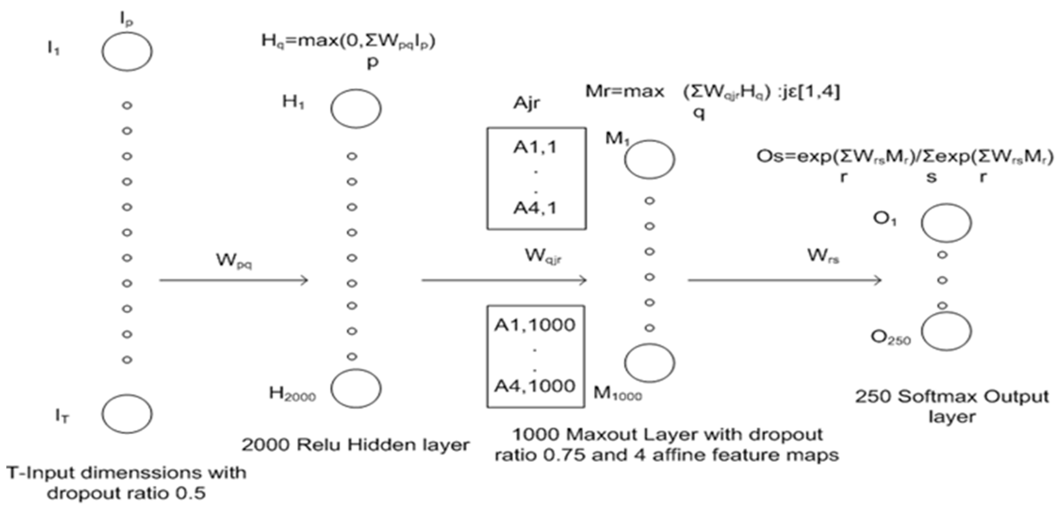
The Adam optimization algorithm is used for optimization [6] of neural network to try to minimize categorical cross entropy as the cost function for 150 iterations using stochastic gradient descent on a mini-batch size of 250 samples. Figure 1 illustrates the proposed neural network architecture graphically. The left-most layer is input layer ‘I’ with dropout ratio 0.5 and dimensions T. H represents the first hidden layer with 2000 neurons and Relu activation. M represents the second hidden layer with Maxout activation and 4 affine maps. O represents the output layer with 250 Softmax units, each representing one of 250 spoken words.

Table 2. Architecture.

Neural Network Architecture

Model Input = Ip = concatenate along 2nd axis (R2500 X Lm, R2500 X 972): pε[1,T] Hidden layer units: Hq = max (0,${\displaystyle \sum }_{\mathrm{p}=1}^{\mathrm{T}}\mathrm{Wpq}\ast \mathrm{Ip}$): qε[1,2000], Wpq = RT X 2000 Maxout affine map = Ajr = ${{\displaystyle \sum }}_{\mathrm{q}=1}^{2000}\mathrm{Wqjr}\ast \mathrm{Hq}$ Maxout layer units: Mr = max (Ajr): jε[1,4], rε[1,1000], Wqjr = R2000 X 4 X 1000 Output units: Os = exp $({{\displaystyle \sum }}_{\mathrm{r}=1}^{1000}\mathrm{Wrs}\ast \mathrm{Mr})$/${{\displaystyle \sum }}_{\mathrm{s}=1}^{250}(\exp {{\displaystyle \sum }}_{\mathrm{r}=1}^{1000}\mathrm{Wrs}\ast \mathrm{Mr})$: sε[1,250], Wrs = R1000 X 250

illustrates the architecture of the proposed neural network model mathematically. Mathematical expressions for each layer are outlined.

Six different neural networks with slight variations in the number of units for each layer are used for averaging. Two models with the above mentioned architecture, a 3rd with 2250 hidden and 1150 Maxout units, a 4th with 1750, hidden 850 Maxout units, a 5th with 1500 hidden, 750 Maxout units and a 6th with 1000 hidden and 500 Maxout units are trained. During testing all six models are used to predict the test data and the average of all outputs gives the target probabilities.

Label propagation is initialized with labels against the same training data set partition that is used for training of the neural network. The 21 nearest neighbors are used for label propagation. Test samples predicted with a label probability higher than 0.95 are selected and, among these selected samples, those which are also predicted as the same word by the initially trained neural network are chosen as the confidently predicted test set. These confidently predicted points are added to the initial training set along with their predicted labels as target words. The neural network model is trained again for 15 iterations on the enhanced training set. This further reduces the predicted WER. The model is initially trained on 9 speakers and tested on 1. Then the test set size is increased incrementally to 2, 3, 4 and 5 speakers and the WER is recorded with different training and validation set combinations. These steps are summarized in Algorithm 1.

Algorithm 1

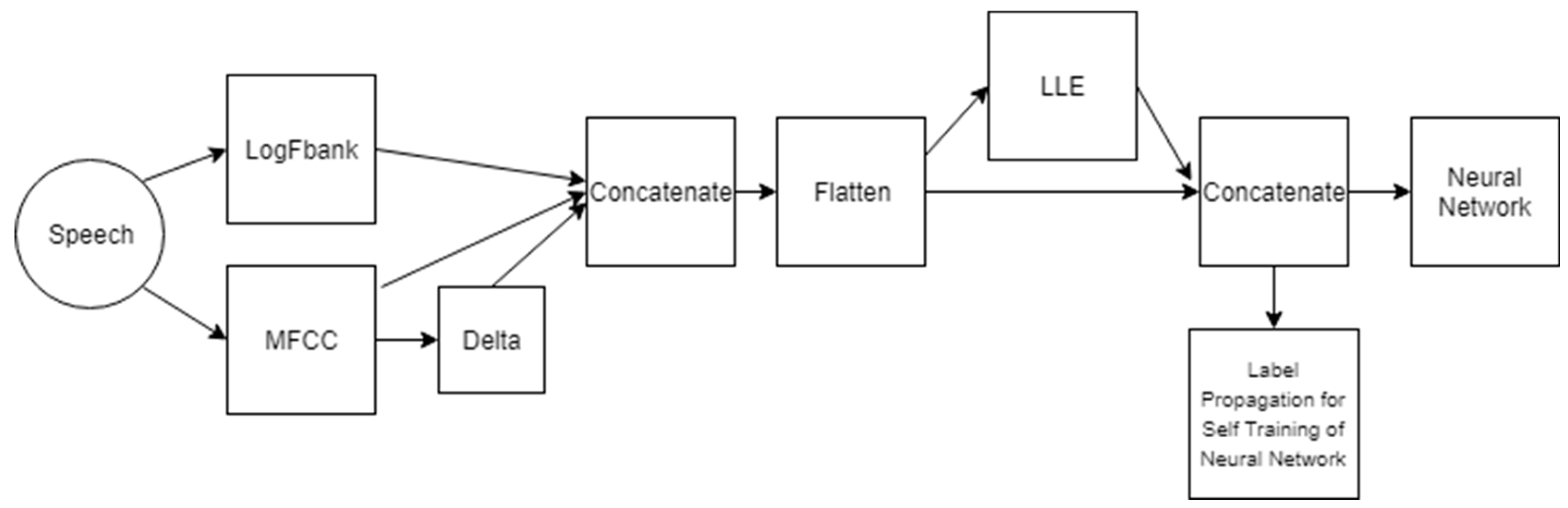
Compute Log Filter Bank, MFCC and Delta coefficients from raw speech Concatenate all coefficients calculated in step 1 Flatten across time into single coefficient vector for each speech sample Extract LLE dimensions from the coefficient matrix of the complete corpus data Concatenate LLE vectors with initial feature vectors Use concatenated vectors as input to the neural network Use same input data for Label Propagation and select confidently labeled samples Self-train neural network with confidently labeled points.

Figure 2 shows a block diagram of the proposed model illustrating the processing steps on raw speech to extract input data for a feed forward neural network with the architecture explained earlier.

4. Results and Analysis

In this section, results of the proposed model are discussed in three directions. First, the effectiveness of the proposed model is analyzed while evaluating the WER. Secondly, the performance of the neural network with different shapes and activation functions is explained. Finally, the impact of self-training and LLE is discussed.

4.1. WER

WER down to 22% is achieved by the proposed SSL-Neural Network (SSL-NN) model for speaker independent setup as compared to 25.42% achieved by HMM on the same corpus [3]. The WER comparison is presented below in

Table 3. Word Error Rate (WER) comparison with Asad-Hidden Markov Models (HMMs) [3].

Train Speakers	Test Speakers	Word Error Rate %
		Asad-HMM [3]	SSL-NN
1–9	0	17.6	35.6
0,2–9	1	20	13.6
0–1,3–9	2	12.8	20
0–2,4–9	3	36.4	17.2
0–3,5–9	4	35	9.6
0–4,6–9	5	13.6	33.2
0–5,7–9	6	38	19.6
0–6,8–9	7	24.8	20
0–7,9	8	26.8	27.2
0–8	9	29.2	24.8
Mean		25.42	22.08

. HMM has better performance for test speakers 0, 2, 5 and 8 while the proposed model predicts better for speakers 1, 2, 3, 4, 6, 7 and 9. Consequently the mean WER of the proposed model is lower than that of HMM.

The HMM model is tested with only 10% data reserved for validation. However, the proposed model is tested to calculate WER with a higher ratio of data from the same corpus reserved as the validation set. Up to 5 speakers are used to test on a model trained with 5 speakers for training. Even after using 2, 3, 4 and 5 speakers as test data, WER does not increase drastically due to unsupervised techniques being incorporated.

Table 4. Mean WER% for different validation dataset size.

Test Set Size	WER %
10%	22.08
20%	22.68
30%	27.34
40%	31.35
50%	34.65

summarizes the mean WER recorded for 20%, 30%, 40% and 50% partition as test data.

WER for different combinations of training and test data are recorded before and after incorporating SSL and model averaging. WER decreases after adding LLE dimensions, it further decreases after self-training using label propagation. Averaging over multiple models reduces WER further. While the lowest WER is obtained after self-training (ST) of ensemble models with LLE appended input data used for training and testing purposes.

Table 5. Word Error Rate for 10% data as test.

Train Speakers	Test Speakers	Word Error Rate %
		Features	Adding LLE	LLE + ST	Ensemble	Ensemble + ST
1–9	0	42	40.4	37.2	37.6	35.6
0,2–9	1	15.6	14.8	12.4	12.8	13.6
0–1,3–9	2	28.4	20.8	21.6	22.8	20
0–2,4–9	3	20.4	18.4	17.2	16.8	17.2
0–3,5–9	4	12.4	10.4	10	9.2	9.6
0–4,6–9	5	36	35.2	34.4	36.4	33.2
0–5,7–9	6	20	21.2	22	18.8	19.6
0–6,8–9	7	25.2	21.6	21.2	20.4	20
0–7,9	8	31.2	30	30.8	29.2	27.2
0–8	9	25.6	26.8	25.6	23.6	24.8
	Mean	25.68	23.96	23.24	22.76	22.08

shows WER details for the validation data set of 1 speaker with neural network trained on 9 speakers after using SSL and averaging.

Table 6. Word Error Rate for 20% data as test.

Train Speakers	Test Speakers	Word Error Rate %
		Features	Adding LLE	LLE + ST	Ensemble	Ensemble + ST
2–9	0,1	30.2	27.8	27.8	26.2	25
0,3–9	1,2	27.2	24	23.2	21.8	21.2
0–1,4–9	2,3	24.8	18.6	18.6	19.4	17
0–2,5–9	3,4	18.2	15.6	15.6	14.4	14.6
0–3,6–9	4,5	26.8	25.8	26	25	23.6
0–4,7–9	5,6	35	32.6	29.6	30.8	28.2
0–5,8–9	6,7	28.6	28.6	25.8	26	23.8
0–6,9	7,8	32	32.2	28.8	27.6	25
0–7	8,9	30.8	30.8	29.8	27	25.8
	mean	28.17	26.22	25.02	24.24	22.68

shows the WER for the validation data set of 2 speakers and the training data of 8 speakers before and after using regularization techniques.

Table 7. Word Error Rate for 30% data as test.

Train Speakers	Test Speakers	Word Error Rate %
		Features	Adding LLE	LLE + ST	Ensemble	Ensemble + ST
3–9	0,1,2	42.26	34.64	34	33.3	30.26
0,4–9	1,2,3	25.46	23.06	21.86	20	20.66
0–1,5–9	2,3,4	24.13	18.133	18.26	18.5	18.4
0–2,6–9	3,4,5	36.4	33.867	29.46	29.7	27.2
0–3,7–9	4,5,6	27.2	28.26	25.33	24.8	22.53
0–4,8–9	5,6,7	36.4	35.734	32.266	32.2	31.2
0-5,9	6,7,8	54.4	34.93	44.93	50	42.8
0–6	7,8,9	32.13	51.067	27.33	27.2	25.73
	Mean	34.79	32.46	29.17	29.46	27.34

shows the WER over the validation data set of 3 speakers. It can be observed that with an increasing validation set size, WER recorded without SSL starts increasing considerably as the corpus data is limited; however, after incorporating SSL, the WER increase is less significant.

Table 8. Word Error Rate for 40% data as test.

Train Speakers	Test Speakers	Word Error Rate %
		Features	Adding LLE	LLE + ST	Ensemble	Ensemble + ST
4–9	0–3,	39.8	31.4	27.7	30.3	26
0,5–9	1–4,	27.7	25.7	26.4	24.5	24.5
0–1,6–9	2–5,	36.8	29.9	30.2	29.6	28.2
1–2,7–9	3–6,	35.5	32	28.5	29.3	27.2
1–3,8–9	4–7,	31.6	32.2	28.8	29.2	27.5
1–4,9	5–8,	56	52.5	46.2	50.9	46.1
1–5	6–9,	44.8	45.8	42.5	42.4	39.3
	mean	38.88	35.64	32.9	33.74	31.25

shows the WER over the validation data set of 4 speakers. It is visible that with an increasing validation data set, the improvement in WER by SSL gets more significant as compared to the smaller validation data partition.

Table 9. Word Error Rate for 50% data as test.

Train Speakers	Test Speakers	WER %
		Features	Adding LLE	LLE + ST	Ensemble	Ensemble + ST
5–9	0–4,	36.4	34.48	33.52	32.64	30.96
0,6–9	1–5,	40.56	37.52	37.2	35.2	32.8
0–1,7–9	2–6,	38.8	30.8	31.52	30.16	28.64
1–2,8–9	3–7,	40.08	37.44	33.12	35.52	32.8
1–3,9	4–8,	50.8	49.6	46.08	45.6	41.84
1–4	5–9,	50.32	47.2	44.32	45.84	40.88
	Mean	42.82	39.5	37.62	37.49	34.65

shows the WER for 5 speakers with the neural network trained on 5 speakers. The WER decreases by 8% using SSL, which is quite significant.

Table 10. Decrease in WER after incorporating Semi-Supervised Learning (SSL) and regularization techniques.

Validation Data	WER% (Simple NN)	WER% (SSL)	WER Decrease
10%	25.68	22.08	3.6
20%	28.17	22.68	5.49
30%	34.79	27.34	7.45
40%	38.88	31.25	7.63
50%	42.82	34.65	8.17

summarizes the WER comparison using Neural Networks (NN) with and without SSL techniques for different numbers of users reserved as the validation set. More significant WER improvement with increasing validation set size demonstrates that SSL is very useful for limited labeled data scenarios, which is the case for low-resource languages like Urdu.

4.2. Neural Network Architecture Analysis

The optimization and generalization of the neural network model are analyzed with Sigmoid, Relu, Leaky Relu and Maxout activations in the hidden layer. Maxout activations give the best results; however, due to multiple affine maps for Maxout, the number of parameters to be optimized is huge. Hence, a lot of memory resources are required. Using the initial hidden layer with Relu activations and stacking Maxout as the 2nd hidden layer reduces resource requirements, as the number of parameters to be optimized decreases due to less inputs to the 2nd hidden layer compared to 1st.

Figure 3 records the optimization of the neural network with the single hidden layer using different activation functions. It can be seen that the neural network with sigmoid activations in the hidden layer converges slower than rectified functions and, among rectified functions, Maxout converges fastest due to its power to adapt with activation shapes, but at the cost of huge resources. Leaky and simple Relu, however, are similar in convergence with less computational resource requirements. 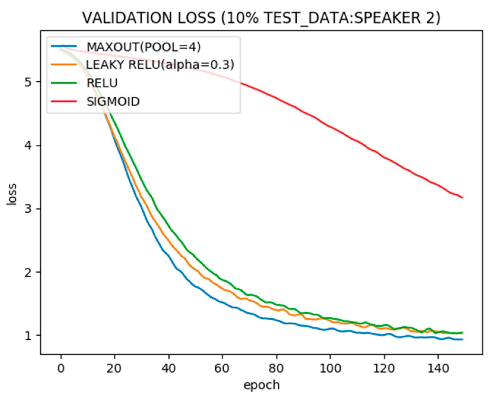Figure 4 shows test error with different activation functions. Again sigmoid shows the worst performance while Maxout is the best. Relu and rectified Relu, however, are almost similar.

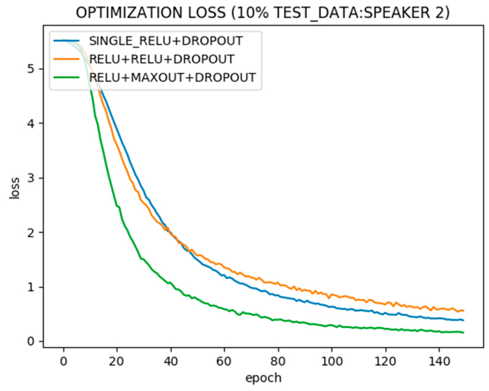
Figure 5 shows optimization convergence of neural networks with single and two hidden layers using different activation functions over the training data of 9 speakers. The optimization is plotted for neural networks with a single Relu hidden layer, two hidden layers, both Relu, and two hidden layers, first Relu and second Maxout. It can be seen that the neural network with two hidden layers, first Relu and second Maxout, converges fastest. 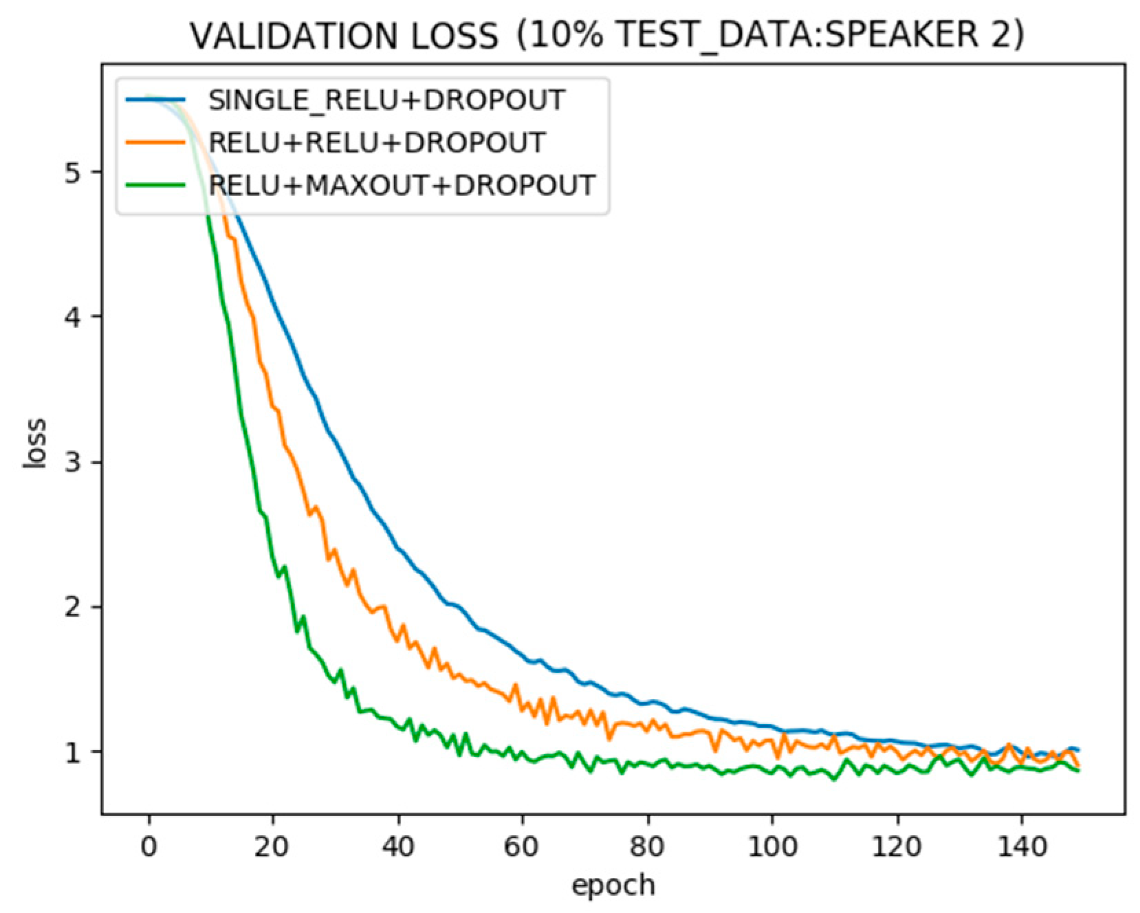Figure 6 shows test error. While all architectures trained on 90% data tend to perform similar on 10% unseen data after steady state, network with Maxout stacked on Relu hidden layer performs better after less iterations of training.

4.3. Evaluation of LLE and Self-Training

The WER keeps decreasing after the self-training of the neural network for 15 iterations using test samples with confidently predicted clusters by label propagation. However, the WER starts to increase after self-training for more iterations as few errors in clustering keep getting emphasized. The optimum of the probability to measure confidence in label propagation clustering is found to be 0.95. For lower cluster probability values, a significant number of samples are added for self-training but more of them include errors, deteriorating the WER. For probability higher than 0.95, a very small set is obtained for self-training, which does not cause significant improvement.

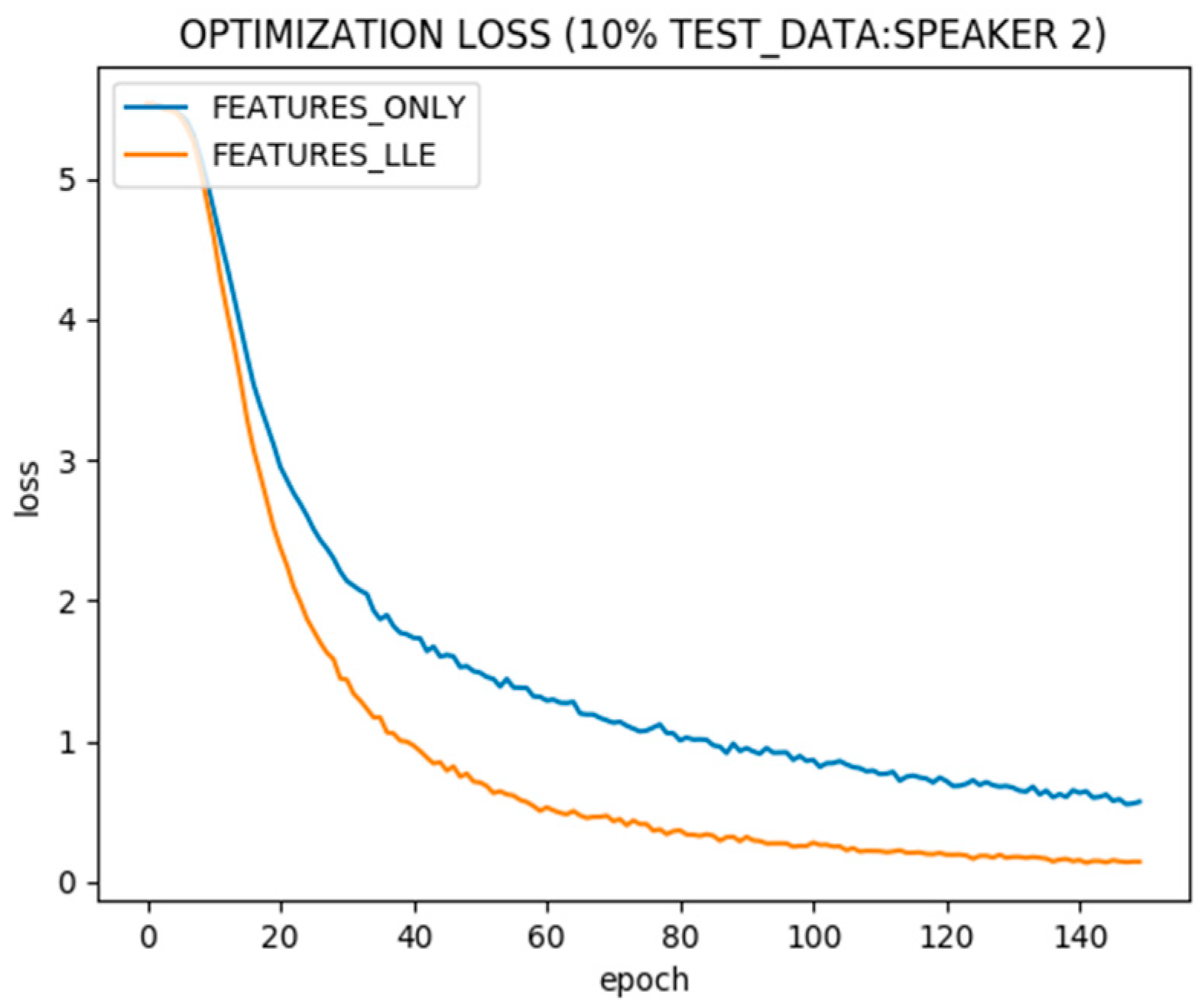
The optimization and generalization of the model are compared before and after adding LLE components to speech features. The optimization improves as LLE helps to extract useful features from the input data set and using structure of both training and test data improves generalization. Figure 7 shows the optimization over 9 speakers’ data used for training with and without adding LLE dimensions to speech features. The optimization is faster using LLE as it extracts key features. 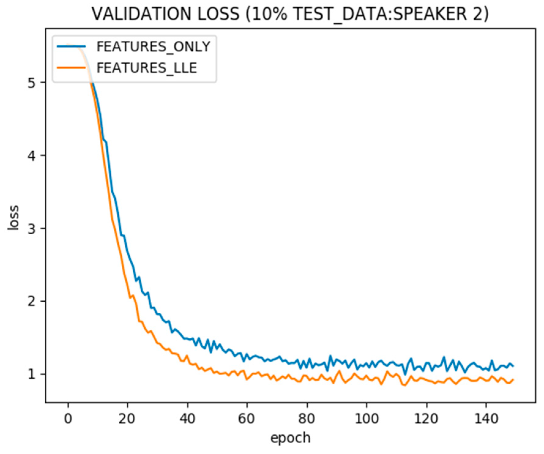Figure 8 shows the test error with and without LLE in the same setting. LLE extracted dimensions appended with speech features improves the steady state validation error on test data due to incorporating the structure of the complete data set, including the test data portion.

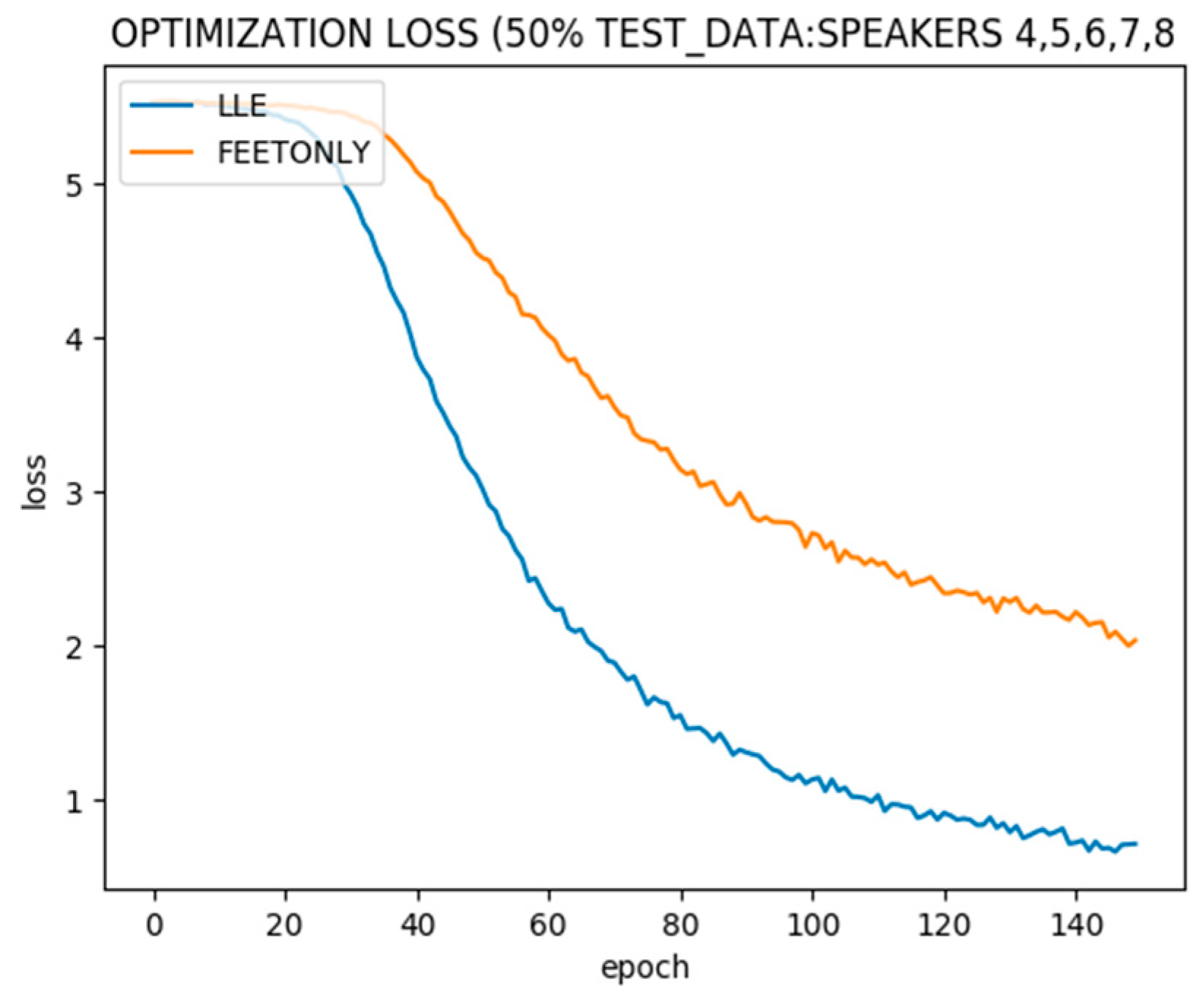
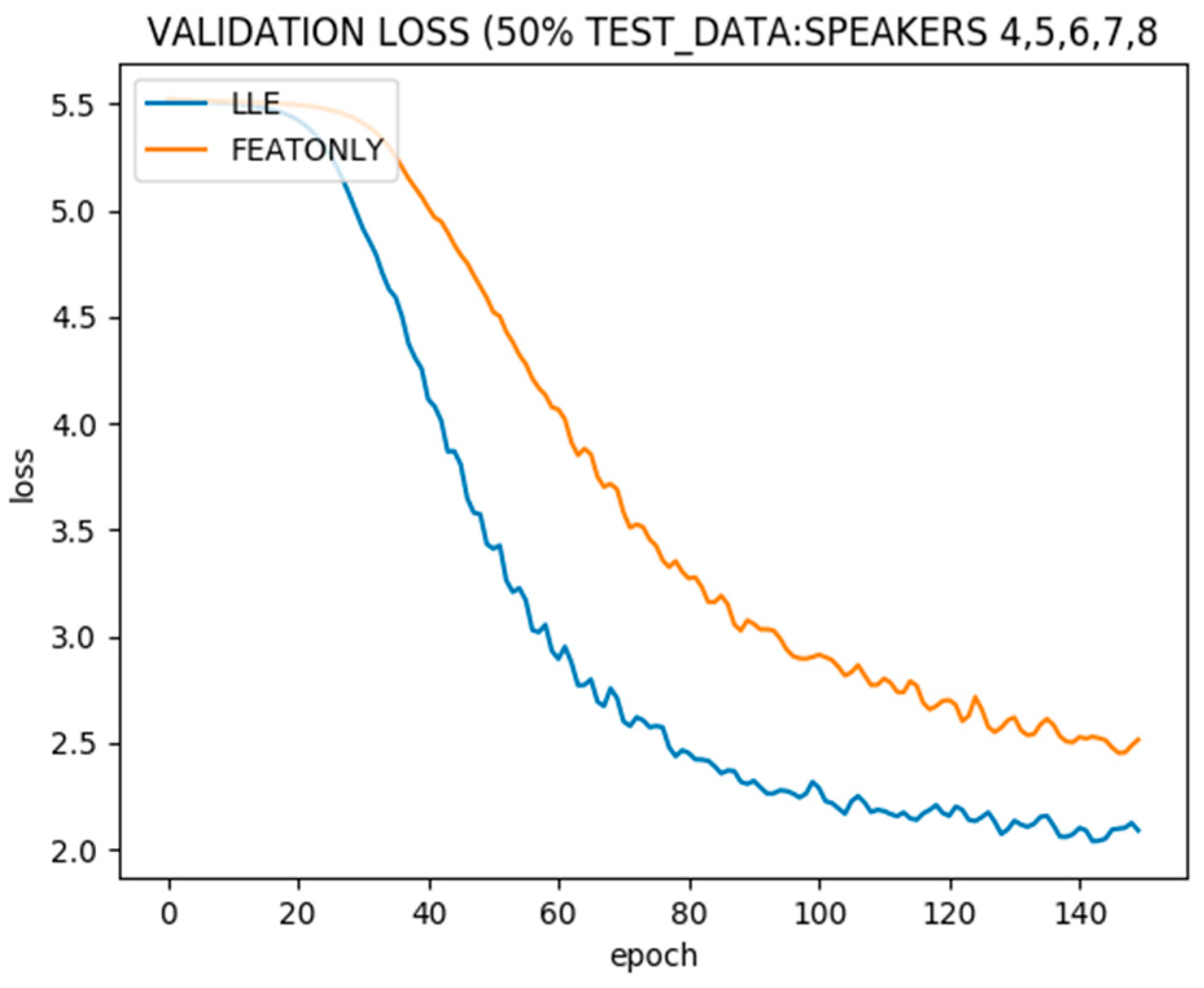
Figure 9 shows the optimization of 5 speakers’ data used for training and 5 speakers reserved as the validation set. LLE extracted dimensions improve optimization. Figure 10 shows the test error in the same setting. With an increase in the unlabeled validation data size, the improvement in generalization after incorporating LLE becomes more significant.

5. Discussion and Conclusions

Due to recent advances in deep learning, neural network-based ASR easily outperforms statistical pattern recognition techniques. Neural networks with Maxout activations in the hidden layer give the best results, but Maxout layers need more memory resources due to the large number of tunable parameters. Memory usage can be reduced by stacking Maxout ahead of the Relu hidden layer. Deep learning regularization techniques, like dropout and model ensembles, reduce WER significantly; however, ensemble over multiple models is resource intensive. Utilizing unsupervised nonlinear dimensionality reduction techniques like LLE improves model generalization for problems with limited labeled data like speech recognition for low-resource languages. SSL techniques like label propagation-based clustering and self-training also reduce WER.

In Future, this work can be extended for Large Vocabulary, Continuous Urdu Speech Recognition. Phoneme-based speech recognition can be used for large vocabulary systems, while state of the art RNNs can be used to incorporate continuous speech. The impact of using discrete time warping DTW distances for extracting speech features, dimensionality reduction and clustering can be explored. LLE and label propagation algorithms can be modified to incorporate DTW distances between speech samples, instead of geographic distance. Incorporating DTW is suitable for variable speed temporal signals like speech. Finally, model robustness can be analyzed using noisy speech samples for training.

References

- Bahdanau, D. End-to-End Attention-based Large Vocabulary Speech Recognition. In Proceedings of the IEEE International Conference on Acoustics Speech and Signal Processing (ICASSP), Shanghai, China, 20–25 March 2016. [Google Scholar]
- Ali, H. A Medium Vocabulary Urdu Isolated Words Balanced Corpus for Automatic Speech Recognition. In Proceedings of the International Conference on Electronics Computer Technology, Kanyakumari, India, 6–8 April 2012. [Google Scholar]
- Shaukat, A.; Ali, H.; Akram, U. Automatic Urdu Speech Recognition using Hidden Markov Model. In Proceedings of the International Conference on Image, Vision and Computing (ICIVC), Portsmouth, UK, 3–5 August 2016. [Google Scholar]
- Bengio, Y. On the Expressive Power of Deep Architectures. In Proceedings of the International Conference on Algorithmic Learning Theory, Espoo, Finland, 5–7 October 2011. [Google Scholar]
- Sutskever, I.; Martens, J.; Dahl, G.; Hinton, G. On the importance of initialization and momentum in deep learning. In Proceedings of the International Conference on Machine Learning, Atlanta, GA, USA, 16–21 June 2013. [Google Scholar]
- Kingma, D.P.; Ba, J. ADAM: A method for stochastic optimization. In Proceedings of the ICLR, San Diego, CA, USA, 7–9 May 2015. [Google Scholar]
- Maas, A.L.; Hannun, A.Y.; Ng, A.Y. Rectifier nonlinearities improve neural network acoustic models. In Proceedings of the International Conference on Machine Learning (ICML), Atlanta, GA, USA, 16–21 June 2013. [Google Scholar]
- Goodfellow, I.J. Maxout networks. arXiv 2013, arXiv:1302.4389. [Google Scholar]
- Li, H.; Wang, X.; Ding, S. Research and development of neural network ensembles: A survey. Artif. Intell. Rev. 2018, 49, 455–479. [Google Scholar] [CrossRef]
- Srivastava, N.; Hinton, G.; Krizhevsky, A.; Sutskever, I.; Salakhutdinov, R. Dropout: A simple way to prevent neural networks from overfitting. J. Mach. Learn. Res. 2014, 15, 1929–1958. [Google Scholar]
- Schwenker, F.; Trentin, E. Pattern classification and clustering: A review of partially supervised learning approaches. Pattern Recogn. Lett. 2014, 37, 4–14. [Google Scholar] [CrossRef]
- Wagstaff, K.; Cardie, C.; Rogers, S.; Schrödl, S. Constrained K-means Clustering with Background Knowledge. In Proceedings of the International Conference on Machine Learning, Williamstown, MA, USA, 28 June–1 July 2001. [Google Scholar]
- Belkin, M.; Niyogi, P. Semi-supervised learning on Riemannian manifolds. Mach. Learn. 2004, 56, 209–239. [Google Scholar] [CrossRef]
- Lasserre, J.A.; Bishop, C.M.; Minka, T.P. Principled Hybrids of Generative and Discriminative Models. In Proceedings of the IEEE Computer Society Conference on Computer Vision and Pattern Recognition, New York, NY, USA, 17–22 June 2006. [Google Scholar]
- Triguero, I.; García, S.; Herrera, F. Self-labeled techniques for semi-supervised learning: Taxonomy, software and empirical study. Knowl. Inf. Syst. 2015, 42, 245–284. [Google Scholar] [CrossRef]
- Zhu, X.; Ghahramani, Z. Learning from Labeled and Unlabeled Data with Label Propagation; Technical Report CMU; Carnegie Mellon University: Pittsburgh, PA, USA, 2002. [Google Scholar]
- Sahraeian, R. Under-Resourced Speech Recognition Based on the Speech Manifold. In Proceedings of the 16th Annual Conference of the International Speech Communication Association, Dresden, Germany, 6–10 September 2015. [Google Scholar]
- Roweis, S.T.; Saul, L.K. Nonlinear Dimensionality Reduction by Locally Linear Embedding. Science 2000, 290, 2323–2326. [Google Scholar] [CrossRef] [PubMed] [Green Version]
© 2019 by the authors. Licensee MDPI, Basel, Switzerland. This article is an open access article distributed under the terms and conditions of the Creative Commons Attribution (CC BY) license (http://creativecommons.org/licenses/by/4.0/).