An Ensemble CNOP Method Based on a Pre-Screening Mechanism for Targeted Observations in the South China Sea

Abstract

The uncertainty in the initial condition seriously affects the forecasting skill of numerical models. Targeted observations play an important role in reducing uncertainty in numerical prediction. The conditional nonlinear optimal perturbation (CNOP) method is a useful tool for studying adaptive observation. However, the traditional CNOP method highly relies on the adjoint model, and it is difficult to find the global optimal solution. In this paper, a pre-screening and ensemble CNOP hybrid method called PECNOP is proposed to identify optimal sensitive areas in targeted observations. PECNOP is an adjoint-free method that captures global CNOP with high probability, which can effectively solve the two major problems faced by traditional CNOP methods. We evaluated the performance of PECNOP by building an observation simulation system consisting of an ocean model and data assimilation. One of the assimilation experiments was dedicated to evaluating the stability and effectiveness of PECNOP in extreme events. The results show that, compared with traditional methods, PECNOP can stably capture the global CNOP. Extra observations and assimilation in the optimal sensitive areas identified by PECNOP can effectively improve forecasting by about 20% within 30 days. Therefore, PECNOP has potential to reduce the initial error of numerical models, which is important for improving forecasting.

1. Introduction

Incorporating large amounts of observation data into ocean numerical models through data assimilation is becoming increasingly important for improving forecasting skills [1,2,3,4,5]. It is well known that various errors can directly affect forecasting skill, such as the initial values, dynamic frameworks, and parameterization schemes. Among them, the uncertainty of the initial value has a particularly critical impact on forecasting skill. In order to improve the quality of the initial value, data assimilation and extra observations are considered effective solutions [6,7,8,9,10,11]. However, ocean observations are extremely difficult and expensive to obtain [12]. Therefore, it is necessary to determine how to obtain observations that most significantly improve the quality of the initial value. In order to solve this problem, adaptive observation (or targeted observations) is proposed. The targeted observations are seen as a major contribution to ocean forecasting [13]. The core of targeted observations is to identify the optimal sensitive area (OSA). In other words, the forecasting skill will be greatly improved by reducing the initial value error at the OSA [14].

A series of studies have been devoted to the design of methods for identifying OSA, summarized into two categories: based on the growth rate of initial error and based on the effect of data assimilation. The first category is designed to capture the most sensitive initial errors, which have the greatest impact on forecasting skill. With these methods, large-value regions with high concentrations of initial errors are identified as OSA. Representative works include linear singular vectors (LSV) [15], sensitivity vectors [16], ensemble sensitivity methods [17], and conditional nonlinear optimal perturbation (CNOP) methods [18]. Among them, the LSV is designed based on linear theory; thus, the OSA of the LSV is reasonable in nonlinear systems only when the forecast moment is short and the amplitude of the initial perturbation is sufficiently small. In order to overcome the limitations of the linear assumption, the conditional nonlinear optimal perturbation (CNOP) method is proposed. The CNOP describes the initial perturbation that satisfies a certain constraint at the moment of prediction and causes a maximum prediction error. The CNOP extends LSV to nonlinear systems [13,19]. However, it is necessary for the adjoint model to be employed in the calculation of CNOP; therefore, the computational cost is relatively high. In addition, the limitations of gradient optimization make it easy for the CNOP to obtain local rather than global optimal solutions. The core of the second category is to employ data assimilation methods to find the area with the largest assimilation correction rate [20]. In the second category, the method based on the ensemble Kalman filter [21,22] is widely adopted because of its small computational cost and simple program implementation. However, these methods are designed under the linear assumption, which greatly limits their applicability to nonlinear systems. Therefore, the CNOP method is more widely used in numerical models.

However, there are some challenges in its operational applications. The essence of the CNOP method is a nonlinear optimization problem. So, the default approach to solving this problem is based on the adjoint model. However, it is notoriously expensive to develop and maintain the adjoint model. In addition, adjoint models of numerical models are often incompatible [18], which severely limits the promotion of CNOP [23,24,25]. To alleviate the dependency of using adjoint models, a CNOP-4DVar hybrid method was proposed [26] based on the CNOP [27,28] and 4DVar (four-dimensional variational) [29]. This hybrid approach is simple to implement and adjoint-free, but the computational cost is also high. Wang et al. [30] proposed an ensemble-based method to approximate the adjoint models called EN-CNOP. The EN-CNOP method can avoid writing adjoint model codes and is equivalent to the CNOP method. However, EN-CNOP still cannot improve the probability of identifying global CNOP.

In general, when faced with complex ocean numerical models, there are often multiple local minimum values in the cost function [31,32,33]. In the context of limited computing resources, the above methods can only capture the global CNOP with a small probability. To solve this problem, Pires et al. [34] proposed the quasi-static variational assimilation (QSVA) technique. However, the computational cost of this method gradually increases as the prediction time increases. Tian et al. [27] proposed a two-step optimization strategy based on the EN-CNOP, and the results showed that a better initial guess can improve the accuracy of calculating global CNOP. However, in practice, in order to reduce the computation time, the initial guess in the two-step optimization strategy is usually randomly selected, which is called random initial guess CNOP (RIG-CNOP). Liu et al. [35] proposed a new scheme based on initial guess pre-analysis (PAIG-CNOP) to obtain global CNOP. The results show that PAIG-CNOP can significantly improve the probability of identifying global CNOP and has low computational cost, but it has not yet been transplanted into a real numerical model.

In summary, adjoint model dependence and non-global CNOP are two key issues. In our study, we designed a pre-screening and ensemble CNOP (PECNOP) method to improve the probability of obtaining the global CNOP and transplant it into a real ocean numerical model. We drew upon experience from the research on analytical four-dimensional ensemble variational data assimilation (A-4DEnVar) [36] and PAIG-CNOP. The algorithm of A-4DEnVar is employed to implement adjoint-free, and PAIG-CNOP is employed to screen the optimal initial guess. An improved multi-scale variational assimilation (MG-3DVar) method can also be organically combined with PECNOP. This hybrid method simultaneously solves the problems of adjoint dependence and local CNOP. The results show the feasibility and stability of the PECNOP, which has certain value in identifying the global CNOP, optimizing the initial value of the numerical model, and improving forecasting skill.

The rest of this paper is organized as follows: In Section 2, we present the theoretical details and workflow of the PECNOP method. We also introduce two basic components (the ocean numerical model and data assimilation method) in the follow-up tests. Section 3 outlines the conducted preliminary experiments and evaluations of the PECNOP method. The assimilation twin experiment was carried out to interpret the characteristics and properties of the OSA in targeted observations from the perspective of data assimilation. At the same time, the effectiveness of pre-screening was explored. In particular, we evaluated the stability of PECNOP in identifying OSAs in extreme events. The paper is concluded in Section 4.

2. Methodology

2.1. Original Definition of CNOP

CNOP describes the initial perturbation that satisfies certain constraints and causes the largest prediction error at the moment of prediction. The original definition of the CNOP method was proposed by Mu and Duan [18]. The following is a brief introduction to CNOP. Suppose the ocean numerical model can be simplified as follows:

$$\left\{\begin{array}{c}\frac{d\mathrm{X}}{dt}=F(\mathrm{X},t)\\ {\left.\mathrm{X}\right|}_{t=0}={\mathrm{X}}_0\end{array}\right.$$

(1)

where $F$ is the nonlinear operator of the numerical model, representing a nonlinear system. The $\mathrm{X}$ is a state variable, including temperature, salinity, etc.; $t$ is a time variable and ${\mathrm{X}}_0$ represents the state at $t=0$ initial state. On the basis of Equation (1), we can further transform the problem as follows:

$${\mathrm{X}}_T={\left.\mathrm{X}\right|}_{t=T}={\mathrm{M}}_{0\to T}({\mathrm{X}}_0)$$

(2)

where $\mathrm{M}$ is an evolution operator controlled by the integration time and the initial state. ${\mathrm{M}}_{0\to T}$ means integrating from the initial moment to the $T$ moment. ${\mathrm{X}}_T$ describes the evolution result of the initial state ${\mathrm{X}}_0$ at the $T$ moment. Let $x_0$ be the initial guess value of CNOP and $x_T$ be the nonlinear evolution of $x_0$ at the $T$ moment, given by:

$$x_T={\mathrm{M}}_{0\to T}(X_0+x_0)-{\mathrm{M}}_{0\to T}({\mathrm{X}}_0)$$

(3)

In order to construct constraints, we need to choose an appropriate norm $‖·‖$ and define the CNOP cost function as:

$$I(x_0)={‖{\mathrm{M}}_{0\to T}({\mathrm{X}}_0+x_0)-{\mathrm{M}}_{0\to T}({\mathrm{X}}_0)‖}^2$$

(4)

where $I(x_0)$ represents the difference of nonlinear development when the initial perturbation is $x_0$. In general, $x_0$ satisfies the initial constraint $‖x_0‖\le \beta$ and maximizing $I(x_0)$ in Equation (4) is written as $x_0^{\ast }$, which is CNOP as follows:

$$I(x_0^{\ast })=\underset{‖x_0‖\le \beta }{\max }{‖{\mathrm{M}}_{0\to T}({\mathrm{X}}_0+x_0)-{\mathrm{M}}_{0\to T}({\mathrm{X}}_0)‖}^2$$

(5)

where $\beta$ is used to constrain the norm distance of $x_0$.

2.2. Design of Pre-Screening and Ensemble CNOP Method

As shown in Figure 1, the overall structure of PECNOP is divided into two parts: the ensemble CNOP (EN-CNOP) core (Figure 1a) and the pre-screening mechanism (Figure 1b). Among them, the EN-CNOP core is an adjoint-free CNOP solution scheme, which can approximate a complex adjoint matrix with ensemble samples. The pre-screening mechanism generates a series of initial guesses and performs only one step of optimization to obtain the optimal initial guess value of the global CNOP.

2.2.1. The Algorithm of the EN-CNOP Core

As shown in Equation (5), the core of CNOP is to solve a constrained maximization problem. However, the current mainstream optimization algorithms are almost all designed to solve the minimization problem, so we replace the CNOP cost function with the reciprocal form and rewrite Equation (4) as:

$$J(x_0)=1/{‖{\mathrm{M}}_{0\to T}({\mathrm{X}}_0+x_0)-{\mathrm{M}}_{0\to T}({\mathrm{X}}_0)‖}^2$$

(6)

The gradient of the cost function with respect to the initial perturbation $x_0$ can be expressed as follows (according to the matrix calculus):

$$\nabla J(x_0)=\frac{-2{\mathrm{M}}_{0\to T}^{\mathrm{T}}({\mathrm{X}}_0+x_0)[{\mathrm{M}}_{0\to T}({\mathrm{X}}_0+x_0)-{\mathrm{M}}_{0\to T}({\mathrm{X}}_0)]}{{‖{\mathrm{M}}_{0\to T}({\mathrm{X}}_0+x_0)-{\mathrm{M}}_{0\to T}({\mathrm{X}}_0)‖}^4}$$

(7)

where ${\mathrm{M}}_{0\to T}^{\mathrm{T}}$ is the transpose of the Jacobian matrix of ${\mathrm{M}}_{0\to T}$, which generally has to be computed from the corresponding adjoint model [37].

An ensemble-based method for obtaining approximate gradients is created as follows. First, a series of uncorrelated initial small perturbations ${\tilde{x}}_i=({\tilde{x}}_1,{\tilde{x}}_2,\cdot \cdot \cdot ,{\tilde{x}}_n)$ is generated. The incremental matrix ${\tilde{y}}_i=({\tilde{y}}_1,{\tilde{y}}_2,\cdot \cdot \cdot ,{\tilde{y}}_n)$ at the prediction moment $T$ corresponding to the ${\tilde{x}}_i$ is obtained as follows (results with perturbation minus results without perturbation):

$${\tilde{y}}_i={\mathrm{M}}_{0\to T}({\mathrm{X}}_0+x_0+{\tilde{x}}_i)-{\mathrm{M}}_{0\to T}({\mathrm{X}}_0+x_0),i=1,2,\cdots ,n$$

(8)

If each member of ${\tilde{x}}_i$ is sufficiently smaller than ${\mathrm{X}}_0+x_0$ and the integration time is short, a first-order linear approximate statistical relationship between ${\tilde{x}}_i$ and ${\tilde{y}}_i$ can be established (according to the Taylor series expansion):

$${\tilde{y}}_i={\mathrm{M}}_{0\to T}({\mathrm{X}}_0+x_0){\tilde{x}}_i,i=1,2,\cdots ,n$$

(9)

Then, we refer to related concepts in the A-4DEnVar [31]; the background state variables error covariance matrix at $t_0$ is ${\mathrm{B}}_{00}=E\left\{{\tilde{x}}_i{\tilde{x}}_i^{\mathrm{T}}\right\}$, where $E\left\{·\right\}$ is the mathematical expectation. According to Equation (9), the error covariance matrix of ${\mathrm{B}}_{T0}$ and ${\mathrm{B}}_{0T}$ can be constructed as follows:

$$\left\{\begin{array}{c}{\mathrm{B}}_{T0}=E\left\{\left.{\tilde{y}}_i{\tilde{x}}_i^{\mathrm{T}}\right\}={\mathrm{M}}_{0\to T}({\mathrm{X}}_0+x_0){\mathrm{B}}_{00}\right.\\ {\mathrm{B}}_{0T}=E\left\{\left.{\tilde{x}}_i{\tilde{y}}_i^{\mathrm{T}}\right\}={\mathrm{B}}_{00}{\mathrm{M}}_{0\to T}^{\mathrm{T}}({\mathrm{X}}_0+x_0)\right.\end{array}\right.$$

(10)

The two background error covariance matrices contain the tangent linear evolution operator matrix ${\mathrm{M}}_{0\to T}$ and the corresponding adjoint operator matrix ${\mathrm{M}}_{0\to T}^{\mathrm{T}}$, respectively. According to Equation (10), the adjoint matrix can be expressed as:

$${\mathrm{M}}_{0\to T}^{\mathrm{T}}({\mathrm{X}}_0+x_0)={\mathrm{B}}_{00}^{-1}{\mathrm{B}}_{0T}$$

(11)

But in practice, we found that the real numerical model of the atmosphere or ocean has a huge dimension, which leads to a very large dimension of ${\mathrm{B}}_{00}$. So, ${\mathrm{B}}_{00}^{-1}$ is difficult to calculate. Therefore, PECNOP constructs the pseudo-inverse and simplifies the computation by matrix orthogonal decomposition [38].

$$\left\{\begin{array}{c}{\tilde{x}}_i{\tilde{x}}_i^{\mathrm{T}}=\begin{array}{c}\mathrm{\Phi }\mathrm{\Lambda }{\mathrm{\Phi }}^{\mathrm{T}}\end{array}\\ {\tilde{x}}_i^{\mathrm{T}}{\tilde{x}}_i=\tilde{\mathrm{\Phi }}\tilde{\mathrm{\Lambda }}{\tilde{\mathrm{\Phi }}}^{\mathrm{T}}\end{array}\right.$$

(12)

As shown in Equation (12), $\mathrm{\Phi }$ and $\tilde{\mathrm{\Phi }}$ represent feature vectors, and $\mathbf{\Lambda }$ and $\tilde{\mathrm{\Lambda }}$ are feature values. Therefore, Equation (11) can be equivalently expressed as (according to the linear transformation of the matrix):

$$\begin{array}{ll}{\mathrm{M}}_{0\to T}^{\mathrm{T}}(X_0+x_0)& ={\mathrm{B}}_{00}^{-1}{\mathrm{B}}_{0T}\\ & ={({\tilde{x}}_i{\tilde{x}}_i^{\mathrm{T}})}^{-1}\left({\tilde{x}}_i{\tilde{y}}_i^{\mathrm{T}}\right)\\ & ={\tilde{x}}_i\tilde{\mathrm{\Phi }}{\tilde{\mathrm{\Lambda }}}^{-2}{\tilde{\mathrm{\Phi }}}^{\mathrm{T}}{\tilde{x}}_i^{\mathrm{T}}{\tilde{x}}_i{\tilde{y}}_i^{\mathrm{T}}\\ & ={\tilde{x}}_i\tilde{\mathrm{\Phi }}{\tilde{\mathrm{\Lambda }}}^{-2}{\tilde{\mathrm{\Phi }}}^{\mathrm{T}}{\tilde{\mathrm{\Phi }}\tilde{\mathrm{\Lambda }}\tilde{\mathrm{\Phi }}}^{\mathrm{T}}{\tilde{y}}_i^T\\ & ={\tilde{x}}_i{\tilde{\mathrm{\Phi }}\tilde{\mathrm{\Lambda }}}^{-1}{\tilde{\mathrm{\Phi }}}^{\mathrm{T}}{\tilde{y}}_i^{\mathrm{T}}\end{array}$$

(13)

Equation (7) can be equivalently expressed as follows:

$$\nabla J(x_0)=\frac{-2{\tilde{x}}_i{\tilde{\mathrm{\Phi }}\tilde{\mathrm{\Lambda }}}^{-1}{\tilde{\mathrm{\Phi }}}^{\mathrm{T}}{\tilde{y}}_i^{\mathrm{T}}[{\mathrm{M}}_{0\to T}({\mathrm{X}}_0+x_0)-{\mathrm{M}}_{0\to T}({\mathrm{X}}_0)]}{{‖{\mathrm{M}}_{0\to T}({\mathrm{X}}_0+x_0)-{\mathrm{M}}_{0\to T}({\mathrm{X}}_0)‖}^4}$$

(14)

So far, EN-CNOP has freed the calculation of the gradient from the adjoint model. Equations (6) and (14) denote the cost function $J(x_0)$ and gradient $\nabla J(x_0)$ of EN-CNOP, respectively. Through the iteration of the optimization algorithm, the CNOP can be obtained at the minimum value of $J(x_0)$. The spectral projected gradient 2 (SPG2) [39] algorithm is used in the optimization stage of EN-CNOP.

2.2.2. Pre-Screening Mechanism for Global CNOP

In Section 2.2.1, the EN-CNOP core implements an adjoint-free CNOP solution after determining that the initial guess value is $x_0$. In practice, the method of choosing the initial guess value is very important. The traditional scheme is to randomly select in the constraint range, but there is a risk of falling into a local minimum. In order to ensure that the generated initial guesses have a certain degree of dispersion (to expand the search range), the pre-screening mechanism needs to generate some initial guesses according to certain rules within the constraints and select an optimal initial guess. Figure 1c is the overall flowchart of PECNOP. The specific implementation of the pre-screening mechanism can be divided into the following four steps:

1.

$H$ groups of $N$ initial guesses $x_0^{H\times N}$ are randomly generated. Each initial guess $x_0^{i,j}$ is generated within the range $(-R_{ij},R_{ij})$, where $R_{ij}$ is expressed as:

$$R_{ij}=\frac{(N-i)}{N}·{\beta }_{\max }+\frac{i}{N}·{\beta }_{\min },(i=1,2,\cdots ,H;j=1,2,\cdots ,N)$$

(15)

where ${\beta }_{\max }={10}^{-i+1}\times \beta$ and ${\beta }_{\min }={10}^{-i}\times \beta ,(i=1,2,\cdots ,H)$. Such a scheme can generate initial guesses for multiple candidates that are as different as possible.

2.

Then, the gradient of the initial guess $x_0^{i,j}$ for each group is computed by Equation (14) of the EN-CNOP core:

$$\nabla J(x_0^{i,j})=\frac{-2{\tilde{x}}_i{\tilde{\mathrm{\Phi }}\tilde{\mathrm{\Lambda }}}^{-1}{\tilde{\mathrm{\Phi }}}^{\mathrm{T}}{\tilde{y}}_i^{\mathrm{T}}[{\mathrm{M}}_{0\to T}({\mathrm{X}}_0+x_0^{i,j})-{\mathrm{M}}_{0\to T}({\mathrm{X}}_0)]}{{‖{\mathrm{M}}_{0\to T}({\mathrm{X}}_0+x_0^{i,j})-{\mathrm{M}}_{0\to T}({\mathrm{X}}_0)‖}^4}$$

(16)

3.

After obtaining the gradient information of all initial guesses, only one optimal search iteration is performed for $x_0^{i,j}$. Then, the updated initial guesses ${x^{\prime }}_0^{i,j}$ and the cost function value (CFV) corresponding to each initial guess can be obtained:

$$J({x^{\prime }}_0^{i,j})=1/{‖{\mathrm{M}}_{0\to T}({\mathrm{X}}_0+x_0^{i,j})-{\mathrm{M}}_{0\to T}({\mathrm{X}}_0)‖}^2$$

(17)

4.

A point $x_0^{\ast }$ is screened out so that the following equation holds (the smallest CFV):

$$J(x_0^{\ast })=\underset{x_0^{\ast }\in {x^{\prime }}_0}{\min }J({x^{\prime }}_0^{i,j})$$

(18)

Finally, the best initial guess $x_0^{\ast }$ is selected for further optimization calculations. It is worth noting that the pre-screening mechanism only performs optimization once and compares the optimized CFVs. This scheme can find the guess with the most potential among all the updated initial guesses. EN-CNOP employs the optimal initial guess value screened by Equation (18) for multiple iterations and finally obtains the optimal initial perturbation (that is, the OSA).

2.3. Ocean Model and Data Assimilation Method

The assimilation twin experiment is a general method to evaluate the effectiveness of the CNOP in identifying OSAs. For this purpose, numerical models and data assimilation methods are necessary. A parallel version of the Princeton Ocean Model with a generalized coordinate system (POMgcs) was employed in our study [40,41]. It uses mixed coordinates on the basis of the original POM [42]. The σ coordinate is used in the upper mixed layer and the shallow sea area, and the z coordinate is used in the cline and lower water layers to improve the vertical resolution. POMgcs uses cutting grids on the seabed, which can more realistically represent the original topography of the seabed, thereby avoiding the ladder effect. The 2.5-order turbulent closure scheme [43] is used to determine the vertical diffusion coefficient of POMgcs.

In the assimilation twin experiment, we employed the multi-grid 3D variational (MG-3DVar) data assimilation method. The multi-grid method was originally developed from the study of the numerical solution of differential equations. In variational data assimilation, the purpose of using the multi-grid method is to quickly correct the long-wave information of the analysis field so as to avoid wrongly transforming long-wave analysis into short-wave analysis. This method [44] uses the grid scale to characterize the different correlation scale features in the background field error covariance matrix and sequentially extracts the information of different wavelengths in the observation data, which solves the problem of the traditional 3DVar only extracting specific wavelength information. In this study, we upgraded the MG-3DVar method to a four-dimensional analysis method, organically combining the horizontal constraints provided by remote sensing and the vertical constraints provided by field observations. In the process of constructing the observation operator of the sea surface height (SSH) anomaly, the dynamical height integral and the sea water state equation are used as natural constraints. A link is established between SSH, sea surface temperature, underwater temperature, and salinity observations. At the same time, this method can effectively extract the multi-scale observation information. An adaptive, more objective, and reasonable temperature–salt analysis field can be obtained by MG-3DVar.

3. Preliminary Experiments

3.1. Experimental Setup

3.1.1. Targeted Region Observations and Data Preparation

In order to better evaluate the effectiveness of the PECNOP, it is necessary to select the appropriate targeted region and object. A representative sea region (Figure 2a), the South China Sea (SCS), was selected as the targeted region for our experiment. The SCS is the largest marginal sea in the Western Pacific, with a maximum depth of more than 5000 m. The SCS western boundary current [45], mesoscale vortex, and air–sea interaction [46] complicate its dynamic evolution. In addition, due to the connection between the SCS and the equatorial Pacific, frequent typhoon events make it more difficult to achieve accurate forecasts in the SCS region. Therefore, the specific region of the preliminary experiment is located between 0° N and 30° N and 100° E and 130° E (Figure 2b). The variables involved in targeted observations include the sea surface height (SSH), three-dimensional temperature, salinity, and ocean currents.

In order to construct the initial guess matrix and the ensemble small perturbation matrix of the CNOP, we employed the reanalysis data product of CORA1.0 (China Ocean ReAnalysis version 1.0). CORA1.0 was also employed to carry out subsequent data assimilation twin experiments. The CORA1.0 product has a horizontal resolution of 1/4° and is vertically divided into 35 layers. Its original spatial coverage is 99° E~150° E and 10° S~52° N, the time range is from 1958 to 2018, and the resolution is daily and monthly. It is worth mentioning that the CORA1.0 product and the ocean dynamic model selected in this study are both POMgcs. In addition, CORA1.0 employs the MG-3DVar to assimilate observations. Therefore, the CORA1.0 product has a natural interface with the experimental configuration of PECNOP.

3.1.2. Initial Configuration of the Ocean Model

In our preliminary experiments, the maximum model depth of POMgcs was 3500 m. There were 14,641 horizontal grid points and 15 vertical layers in our model domain (0° N~30° N, 100° E~130° E). We employed the 1 arc-minute global relief model of Earth’s surface (ETOPO1) from the National Genomics Data Center (NGDC) [47]. The minimum depth of the model was set to 10 m near the shore. The open boundary of this domain was obtained from the monthly average data reanalyzed using Simple Ocean Data Assimilation (SODA) [48]. The initialization of POMgcs was a two-step process: In the first step, a cold start, we integrated the model using the December climate state from the World Ocean Atlas 2005 (WOA05) [49] as the initial temperature and salinity fields. Physical variables such as 10 m wind, 2 m air temperature, relative humidity, total cloud cover, precipitation, runoff, and sea level pressure from the fifth-generation ECMWF atmospheric reanalysis of the global climate (ERA5) reanalysis of the European Centre for Medium-Range Weather Forecasts (ECMWF) [50] monthly average data were used to drive POMgcs. In addition, we combined the above physical variables with the surface current and sea surface temperature data integrated by the model into the block formula of the COARE3.0 [51] algorithm to calculate meteorological driving fields such as long-wave radiation, sensible heat, latent heat, short-wave radiation, and wind stress. After 10 years of spin-up, the upper ocean has basically reached a quasi-equilibrium state [52]. In the second step, we assimilated the daily SSH anomalies, three-dimensional temperature, and salinity data from 1 January 2015 to 31 December 2018. The assimilation results obtained in the second step on 31 December 2018 were used as the initial field for the targeted observation experiment.

In order to construct the true field of the assimilation twin experiment, we employed the GLORYS12V1 product as the “observation data” with the ideal assumption. This is a reanalysis product of CMEMS global ocean eddy resolution (1/12° horizontal resolution and 50 vertical layers). We used the daily assimilation results of 2019 (365 days in total) as the ground truth. Because our follow-up preliminary experiment is an ideal twin experiment, the comprehensive evaluation with the same data assimilation method can directly compare the effect of assimilation inside and outside the optimal OSA.

3.1.3. Experimental Design for Identifying Sensitive Areas

Before executing the PECNOP program, in addition to subtracting the climatic state from the historical reanalysis data to generate a perturbation matrix, we imposed spherical constraints on the generated ensemble perturbations [35], constraining the range of the initial guess value matrix within β (constraint radius). Choosing an appropriate constraint β helps to find the global optimal solution of CNOP. The value of β depends on the stability of the numerical model. If β is too large, the numerical solution will be unstable. At the same time, if β is too small, it will lead to a trivial solution of CNOP. Therefore, under the condition of ensuring the stability of the numerical solution, the β should be selected to be as large as possible.

In order to choose a reasonable constraint β, we compared the impact of different constraints on CNOP. As shown in Figure 3, we performed PECNOP optimization stability experiments of β in the range of 1 × 10⁻⁷ to 5 × 10⁻⁵. It can be seen that when β is too large, PECNOP will stop running after a few iterations, and, especially when β = 5 × 10⁻⁵, PECNOP will be broken after only three steps. When β is too small, PECNOP can run stably, but there are obvious differences in the magnitude of optimization. Therefore, under the premise of ensuring the stability of the numerical solution and optimization efficiency, the value should be selected to be as large as possible. In this study, β was set to 5 × 10⁻⁶.

In calculating the maximum initial error development (CNOP), we perturbed the SSH anomaly ($\tilde{\eta }$), temperature ($\tilde{T}$), salinity ($\tilde{S}$), zonal current velocity ($\tilde{U}$), and meridional current velocity ($\tilde{V}$) in the POMgcs. Thus, the constraint forms of five groups of variable perturbation information are defined:

$$‖x_0‖=\frac{1}{NG}{\displaystyle \sum \sqrt{{(\frac{\tilde{\eta }}{{\eta }_{std}})}^2+{(\frac{\tilde{S}}{S_{std}})}^2+{(\frac{\tilde{T}}{T_{std}})}^2+{(\frac{\tilde{U}}{U_{std}})}^2+{(\frac{\tilde{V}}{V_{std}})}^2}}\le \beta$$

(19)

where (${\eta }_{std}$, $S_{std}$, $T_{std}$, $U_{std}$, $V_{std}$) represents the standard deviation of each variable (calculated from the CORA reanalysis), ($\tilde{\eta }$, $\tilde{S}$, $\tilde{T}$, $\tilde{U}$, $\tilde{V}$) represents the perturbation added to each variable, and NG is the total number of grids in the POMgcs. As shown in Equation (19), the initial perturbation is the average perturbation normalized by the standard deviation of each variable [53]. The L2 norm form in Equation (19) can perform spherical constraints on the perturbation well.

In this experiment, we only added perturbation to shallow areas below 1000 m. As shown in

Table 1. Experimental setup of targeted observations.

Name	Initial Month	Integration Step (Day)	Year of Sample
Case1	January	30	(2015, 2016, 2017)
Case2	April	30	(2014, 2015, 2016)
Case3	July	30	(2013, 2014, 2015)
Case4	October	30	(2012, 2013, 2014)

, in order to obtain statistically significant CNOP results, a total of four groups of experiments were set up. The ensemble perturbation of each group contained three members. It is worth noting that ensemble members have year overlaps but not duplicates. We finally averaged the CNOP results of the four groups to obtain the OSA.

3.2. Experimental Results and Analysis

We conducted preliminary experiments with PECNOP and obtained the OSA of the targeted observation region in Section 3.1. By analyzing the statistical properties of each physical variable in the OSA, we interpreted the mechanism of the OSA from an intuitive perspective (Section 3.2.1). In order to verify the rationality and usability of the OSA, we compared the assimilation effect inside and outside the OSA (Section 3.2.2). The integration window for our statistical evaluation was set to 30 days. To evaluate the stability of PECNOP in extreme events, we analyzed the simulation results during the SCS with a typhoon (DANAS) in Section 3.2.3.

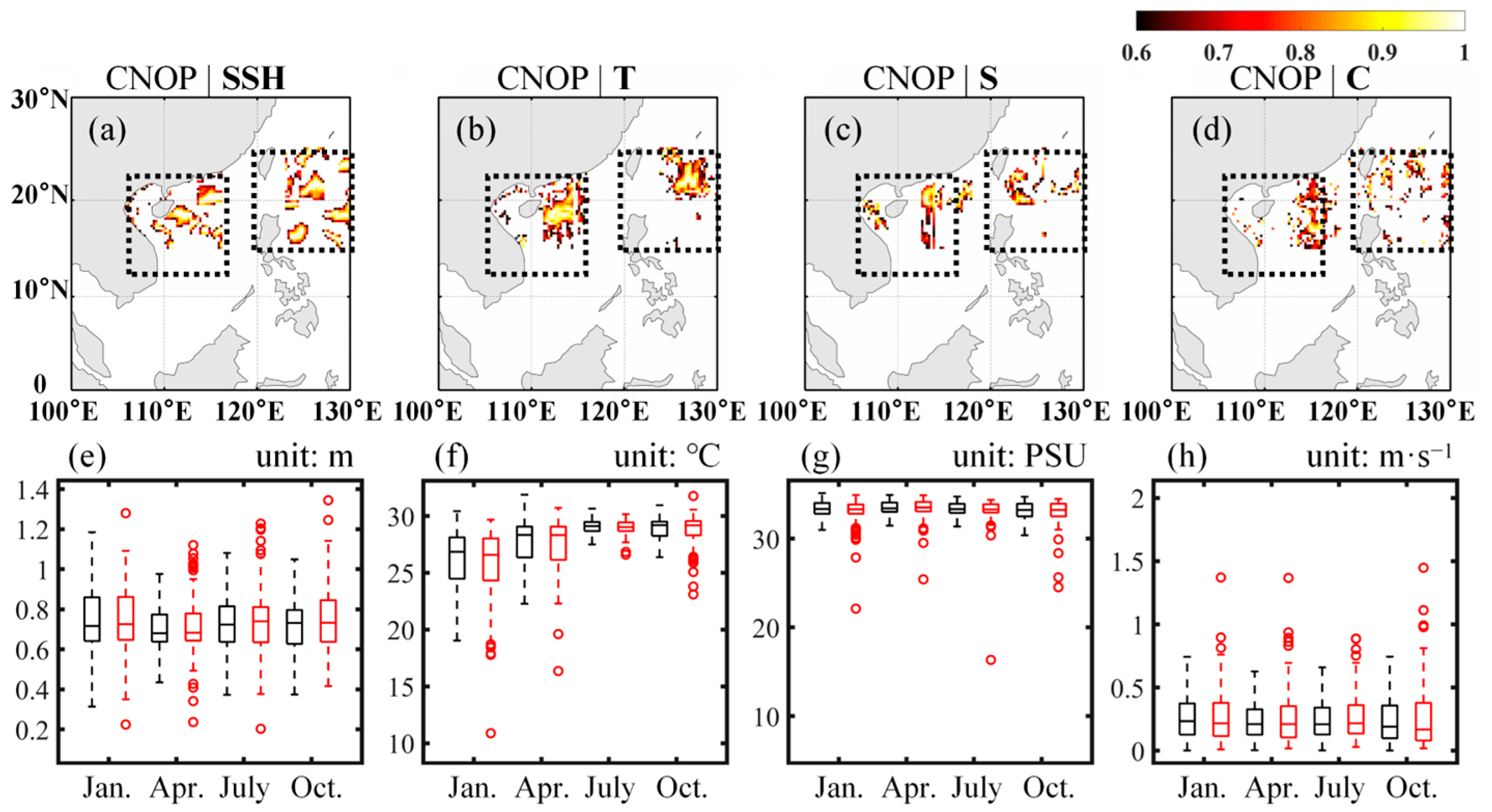
3.2.1. Analysis of Sensitive Areas

PECNOP obtains the CNOP three-dimensional field results of five variables. We vertically integrated the 3D CNOP to obtain the total energy distribution of the five variables. We took the area with total energy greater than 0.6 after normalization as the OSA for the targeted observation. In our experiments, the OSA represented the area of initial perturbation that has the greatest impact on the nonlinear development at the forecast moment. Figure 4 shows the OSA obtained with PECNOP. By integrating the results of different starting months (case1~case4), we found that the OSA of SSH (Figure 4a), temperature (Figure 4b), salinity (Figure 4c), and current velocity (Figure 4d) showed a relatively consistent distribution. There are two significant OSAs near the Paracel Islands (to the west of 120° E) and Taiwan Island (to the east of 120° E). This shows that the development of the initial perturbation in these two areas plays an important role.

As shown in Figure 4e–h, the seasonal evolution within the significant OSA obtained by PECNOP is consistent with that of the entire targeted observation region (TOR). We took temperature as an example (Figure 4f), with the seasonal warming captured by the OSA, and the quantile distributions of the OSA and TOR were almost identical. In comparison, we found that the median temperature in the OSA was slightly lower than that of the TOR, but the difference was <1 °C. It is worth mentioning that OSA tends to pay attention to low-value areas of temperature and salinity, which also leads to the classification of low-temperature and low-salt samples as outliers in statistical comparisons. Meanwhile, the OSA tends to focus on high values of SSH and ocean currents. The SSH statistical results (Figure 4e) of the OSA in April and July show that the evolution of the TOR and OSA shows regular fluctuations. According to the overall statistics, the OSA obtained by PECNOP is consistent with the evolution in the TOR, and the workload required for observation is significantly reduced. Therefore, in this process, the differentiated information in the TOR should be highlighted in the OSA.

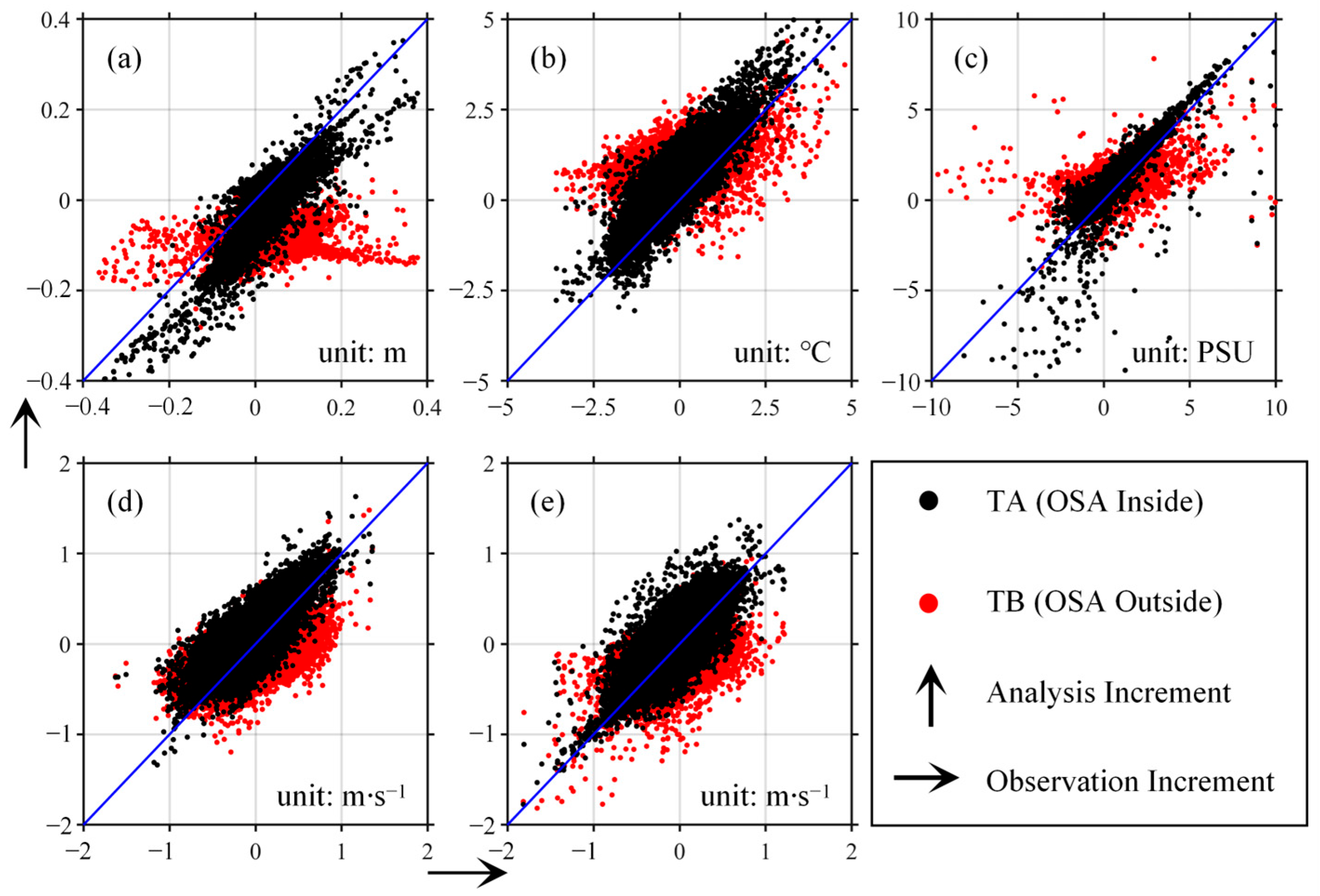
3.2.2. Analysis of the Targeted Assimilation Results

In order to evaluate the impact of the observation data inside the OSA on numerical model forecasting and data assimilation, we compared the performance of assimilation inside and outside the OSA in 2019 (a total of 336 samples). We assimilated pseudo-observations extracted from the ground truth into the initial state and integrated for 30 consecutive days. During these 30 days, our forecasting system did not perform any data assimilation and only relied on the results of initial state assimilation to compare the improvement in the forecast.

Figure 5 shows the comparison results of assimilation inside the OSA (TA) and assimilation outside the OSA (TB) with respect to the ground truth (T0). To show the effect of assimilation, we calculated the difference between the assimilation result and the background field. The forecast results on 15 June 2019 show that the assimilated temperature section (Figure 5b) and salinity section (Figure 5e) in the OSA were closer to the ground truth (the location of the section is shown by the red dotted line in Figure 2b). By comparing Figure 5b,c, we find that assimilation improvements within the OSA are significantly reflected in the region east of 120° E. In the area shallower than 150 m, there is an obvious “low-high-low” band-shaped temperature anomaly distribution. In June, the temperature reached its highest value in 2019, and the slight north–south difference was amplified. In the twin experiment, the difference between the ground truth and the background state of the vertical temperature (Figure 5a) was around −4 °C, which means that the background state overestimates the temperature, while the ground truth shows that it is low. Figure 5b visually shows the improvement in the forecast performance of assimilation within the OSA, where the structure of the banded distribution is captured. Figure 5c shows that assimilation outside the OSA can also improve the forecast performance. In particular, there is a temperature anomaly dipole west of 120° E, which can be captured by both TA and TB. However, east of 120° E, the improvement of the forecast effect by TB is not as obvious as TA. This problem is also evident in the comparison of the salinity section (Figure 5d–f). The above results show that although the OSA is only a small region in the TOR, its assimilation improvement to the initial field is very significant. Therefore, assimilation in the OSA captured by PECNOP can more efficiently improve forecasting.

In order to further evaluate the effectiveness of PECNOP, we analyzed the forecast skills of 336 experimental samples in 2019. Figure 6 and

Table 2. The mean anomaly correlation coefficient (ACC) of different variables in T0 (ground truth), TA (assimilation inside the OSA), and TB (assimilation outside the OSA).

Test Name	SSH	Temperature	Salinity	Current	Mean
T0	0.613	0.517	0.509	0.472	0.527
TA	0.706	0.633	0.636	0.610	0.646
TB	0.673	0.603	0.612	0.568	0.614

reflect the spatial anomaly correlation coefficient (ACC) of assimilation in different regions. It can be seen that the background (T0 in Figure 6) had the lowest ACC with the ground truth. Meanwhile, the ACCs of assimilation inside the OSA (TA) within the OSA were relatively better. As shown by the temperature (Figure 6b), the ACCs of TA and assimilation outside the OSA (TB) decreased to 0.614 and 0.572 on the 15th day of forecast. Compared with T0 (0.508), the assimilation method itself improved the performance of the model forecast, but TA was obviously larger. Taking salinity (Figure 6d) as an example, the ACCs of TA and TB on the 20th day of the forecast were reduced to 0.607 and 0.577, respectively. Compared with T0 (0.494), the assimilation of TA had a greater improvement in the forecast performance.

As shown in Table 2, the mean ACCs of T0 (ground truth), TA (assimilation inside the OSA), and TB (assimilation outside the OSA) were 0.527, 0.646, and 0.614, respectively. The TA was about 22% higher than T0 and about 5% higher than TB. The above results more intuitively show that the OSA has a greater effect on eliminating the initial field error. At the same time, it also indirectly verifies that the PECNOP is effective.

3.2.3. Effectiveness of Pre-Screening Mechanisms

To further evaluate the effectiveness of the pre-screening mechanism, we compared the performance of our PECNOP and EN-CNOP (without pre-screening) in identifying the OSA. It is worth mentioning that the variable dimensions of the numerical model are huge, which makes it impossible for us to verify the uniqueness of the global CNOP through enumeration. Therefore, we can indirectly verify the effectiveness of the pre-screening mechanism by comparing the similarity between OSAs identified by the two methods.

As shown in Figure 7, we set up a total of 10 groups of experiments (EXP1~10). The initial guess value of each group was randomly generated, which can ensure that the distribution of the initial guess value is different. The verification moment of the target observation is 1 October 2019, and temperature was used as an example. We first calculated an optimal sensitive area through the PECNOP method. Then, completely different initial guess values were employed to drive EN-CNOP and PECNOP. As shown in Figure 7a, the correlation coefficient between the OSA identified by PECNOP and the OSA at the target observation moment was significantly higher than that of EN-CNOP. The results of EN-CNOP (Figure 7b) show that the OSA is quite different when the correlation of the initial guess values is low. However, the results of PECNOP (with the pre-screening mechanism) in identifying OSAs are relatively stable (Figure 7c). This is because the CNOP captured by EN-CNOP without pre-screening is the local optimal solution. The role of pre-screening is to expand the sample range of initial guess values, which can increase the probability of capturing global CNOP. Therefore, the pre-screening mechanism is an effective method to capture global CNOP.

3.2.4. Analysis of an Extreme Case

In order to verify the stability of PECNOP, we analyzed the forecast performance in a typhoon event. The SCS is a high incidence area of tropical cyclones. The impact depth of severe typhoons on the ocean can exceed 1000 m [54]. Typhoons cause a series of changes in the ocean, generating huge waves and transporting high heat to the atmosphere and strong surface wind-driven currents [55]. We did not attempt to forecast the typhoon process but rather tested the stability of PECNOP through assimilation twin experiments.

As shown in Figure 8, the No. 5 typhoon “DANAS” in 2019 lasted for 7 days from 15 July to 21 July. 16 July and 18 July, shown in Figure 8a, are two-day examples of DANAS in our TOR. The start date of our experiment was July 15th. After completing the assimilation of the initial state, POMgcs was integrated for 10 days (16 July 2019~25 July 2019). As shown in Figure 8b–e, the central area of DANAS moved to the vicinity of the Kuroshio. The superposition effect intensifies the mixing of subsurface seawater (Figure 8b). The strong sea–air interaction caused the SST near Taiwan Island to fluctuate by about 0.8 °C (Figure 8d), and the change in SSS was about 0.5 PSU (Figure 8e).

We evaluated forecast errors for five surface variables. The mean RMSE (

Table 3. The root mean square error (RMSE) of five surface variables for TA (assimilation inside the OSA) and TB (assimilation outside the OSA).

Name	Metrics	Steps	SSH (m)	SST (°C)	SSS (PSU)	SSU (m·s−1)	SSV (m·s−1)
TA	RMSE	5	0.052	0.332	0.056	0.033	0.038
		10	0.091	0.376	0.068	0.067	0.071
	Mean		0.063	0.351	0.061	0.058	0.062
TB	RMSE	5	0.058	0.353	0.056	0.035	0.043
		10	0.093	0.381	0.071	0.069	0.079
	Mean		0.071	0.367	0.063	0.061	0.066

) of SSH, SST, SSS, SSU, and SSV in TA was 6.3 cm 0.351 °C, 0.061 PSU, 0.058 m·s⁻¹, and 0.063 m·s⁻¹, respectively. The mean RMSE of SSH, SST, SSS, SSU, and SSV in TA was 7.1 cm, 0.367 °C, 0.063 PSU, 0.061 m·s⁻¹, and 0.066 m·s⁻¹, respectively. It can be seen that TA outperformed TB in the RMSE evaluation. In a regression analysis of five variables from 16 to 25 July 2019, we employed R² and adjusted R² to measure the difference between TA (assimilation inside the OSA), TB (assimilation outside the OSA), and the ground truth.

As shown in Figure 9, the regression of the analysis increment to the observation increment was better for TA (inside the OSA) than for TB (outside the OSA).

Table 4. The R² and adjusted R² of five surface variables for TA (assimilation inside the OSA) and TB (assimilation outside the OSA).

Name	Metrics	SSH (m)	SST (°C)	SSS (PSU)	SSU (m·s−1)	SSV (m·s−1)	Mean
TA	R2	0.734	0.747	0.745	0.638	0.593	0.691
	Adj R2	0.731	0.746	0.743	0.633	0.591	0.688
	Mean	0.732	0.746	0.744	0.635	0.592	0.690
TB	R2	0.282	0.317	0.225	0.274	0.216	0.262
	Adj R2	0.281	0.317	0.223	0.272	0.216	0.261
	Mean	0.281	0.317	0.224	0.273	0.216	0.262

presents the R² and adjusted R² of the incremental regression in Figure 9a–e. The mean coefficient of determination of TA was about 0.4 larger than that of TB. This shows that the results of TA assimilation are more stable in the 10-day forecast window and are more consistent with the ground truth.

The above results all show that the extra observations and data assimilation in the OSA captured by PECNOP have greater stability and usability in forecasting tasks in different scenarios.

4. Conclusions

In this paper, we propose a pre-screening and ensemble CNOP hybrid method called PECNOP to identify optimal sensitive areas (OSAs) in targeted observations. The advantage of PECNOP is that it can simultaneously meet the requirements of adjoint-free and high-probability solutions to global CNOP. EN-CNOP is employed to approximate the adjoint model, and pre-screening is employed to generate the optimal initial guess. The results show that PECNOP performs better than the EN-CNOP method, which can capture as much of the global CNOP as possible while improving the computational efficiency. Furthermore, we evaluated the comprehensive performance of the PECNOP method by constructing a targeted observation system combining the ocean model and data assimilation method. At the same time, we designed the assimilation twin experiment of PECNOP. The evaluation results show that PECNOP has stable performance and can capture the global CNOP while reducing the computational cost. The extra observations and assimilation of PECNOP can improve the forecast performance by about 20%. In summary, the targeted observations method based on PECNOP has demonstrated a good ability to capture OSAs in preliminary experiments. PECNOP has great potential to improve the quality of initial states in numerical prediction. More extensive and in-depth exploratory applications can be launched in the future.

Of course, different numerical models and assimilation methods also have a direct relationship with the performance of PECNOP. In practical applications, appropriate models and assimilation methods should be selected according to the requirements to maximize the role of targeted observations. In addition, more factors need to be considered when observing the ocean, such as the observation error and spatiotemporal resolution. PECNOP is still a promising method to improve targeted observations and forecasting. In this study, more complex effects, such as tidal currents, were not considered, which will be one of the core tasks of our future work. The targeted observations scheme for sea–atmosphere coupling and multi-scale forecasting will also be discussed in our future work.

References

1. Rasmusson, E.M.; Carpenter, T.H. Variations in Tropical Sea Surface Temperature and Surface Wind Fields Associated with the Southern Oscillation/El Niño. Mon. Weather. Rev. 1982, 110, 354–384. [Google Scholar] [CrossRef]
2. Philander, S.G.H. El Niño Southern Oscillation Phenomena. Nature 1983, 302, 295–301. [Google Scholar] [CrossRef]
3. Wu, C.-C.; Chou, K.-H.; Lin, P.-H.; Aberson, S.D.; Peng, M.S.; Nakazawa, T. The Impact of Dropwindsonde Data on Typhoon Track Forecasts in DOTSTAR. Weather. Forecast. 2007, 22, 1157–1176. [Google Scholar] [CrossRef]
4. Chou, K.-H.; Wu, C.-C.; Lin, P.-H.; Aberson, S.D.; Weissmann, M.; Harnisch, F.; Nakazawa, T. The Impact of Dropwindsonde Observations on Typhoon Track Forecasts in DOTSTAR and T-PARC. Mon. Weather. Rev. 2011, 139, 1728–1743. [Google Scholar] [CrossRef]
5. Zheng, Q.; Li, W.; Shao, Q.; Han, G.; Wang, X. A Mid- and Long-Term Arctic Sea Ice Concentration Prediction Model Based on Deep Learning Technology. Remote Sens. 2022, 14, 2889. [Google Scholar] [CrossRef]
6. Köhl, A.; Stammer, D. Optimal Observations for Variational Data Assimilation. J. Phys. Oceanogr. 2004, 34, 529–542. [Google Scholar] [CrossRef]
7. Montani, A.; Thorpe, A.J.; Buizza, R.; Undén, P. Forecast Skill of the ECMWF Model Using Targeted Observations during FASTEX. Q. J. R. Meteorol. Soc. 1999, 125, 3219–3240. [Google Scholar] [CrossRef]
8. Lermusiaux, P.F.J. Adaptive Modeling, Adaptive Data Assimilation and Adaptive Sampling. Phys. D Nonlinear Phenom. 2007, 230, 172–196. [Google Scholar] [CrossRef]
9. Shahrezaei, I.H.; Kim, H.-C. A Novel SAR Fractal Roughness Modeling of Complex Random Polar Media and Textural Synthesis Based on a Numerical Scattering Distribution Function Processing. IEEE J. Sel. Top. Appl. Earth Obs. Remote Sens. 2021, 14, 7386–7409. [Google Scholar] [CrossRef]
10. Large, W.G.; McWilliams, J.C.; Doney, S.C. Oceanic Vertical Mixing: A Review and a Model with a Nonlocal Boundary Layer Parameterization. Rev. Geophys. 1994, 32, 363–403. [Google Scholar] [CrossRef]
11. Morss, R.E.; Battisti, D.S. Evaluating Observing Requirements for ENSO Prediction: Experiments with an Intermediate Coupled Model. J. Clim. 2004, 17, 3057–3073. [Google Scholar] [CrossRef]
12. Mu, M. Methods, Current Status, and Prospect of Targeted Observation. Sci. China Earth Sci. 2013, 56, 1997–2005. [Google Scholar] [CrossRef]
13. Mu, M.; Zhou, F.; Wang, H. A Method for Identifying the Sensitive Areas in Targeted Observations for Tropical Cyclone Prediction: Conditional Nonlinear Optimal Perturbation. Mon. Weather. Rev. 2009, 137, 1623–1639. [Google Scholar] [CrossRef]
14. Majumdar, S.J. A Review of Targeted Observations. Bull. Am. Meteorol. Soc. 2016, 97, 2287–2303. [Google Scholar] [CrossRef]
15. Palmer, T.N.; Gelaro, R.; Barkmeijer, J.; Buizza, R. Singular Vectors, Metrics, and Adaptive Observations. J. Atmos. Sci. 1998, 55, 633–653. [Google Scholar] [CrossRef]
16. Langland, R.H.; Gelaro, R.; Rohaly, G.D.; Shapiro, M.A. Targeted Observations in FASTEX: Adjoint-Based Targeting Procedures and Data Impact Experiments in IOP17 and IOP18. Q. J. R. Meteorol. Soc. 1999, 125, 3241–3270. [Google Scholar] [CrossRef]
17. Ancell, B.; Hakim, G.J. Comparing Adjoint- and Ensemble-Sensitivity Analysis with Applications to Observation Targeting. Mon. Weather. Rev. 2007, 135, 4117–4134. [Google Scholar] [CrossRef]
18. Mu, M.; Duan, W.S.; Wang, B. Conditional Nonlinear Optimal Perturbation and Its Applications. Nonlinear Process. Geophys. 2003, 10, 493–501. [Google Scholar] [CrossRef]
19. Zhou, F.; Mu, M. The Impact of Verification Area Design on Tropical Cyclone Targeted Observations Based on the CNOP Method. Adv. Atmos. Sci. 2011, 28, 997–1010. [Google Scholar] [CrossRef]
20. Daescu, D.N.; Navon, I.M. Adaptive Observations in the Context of 4D-Var Data Assimilation. Meteorol. Atmos. Phys. 2004, 85, 205–226. [Google Scholar] [CrossRef]
21. Zhang, Y.; Xie, Y.; Wang, H.; Chen, D.; Toth, Z. Ensemble Transform Sensitivity Method for Adaptive Observations. Adv. Atmos. Sci. 2016, 33, 10–20. [Google Scholar] [CrossRef]
22. Houtekamer, P.L.; Mitchell, H.L. A Sequential Ensemble Kalman Filter for Atmospheric Data Assimilation. Mon. Weather. Rev. 2001, 129, 123–137. [Google Scholar] [CrossRef]
23. Tian, X.; Zhang, H.; Feng, X.; Xie, Y. Nonlinear Least Squares En4DVar to 4DEnVar Methods for Data Assimilation: Formulation, Analysis, and Preliminary Evaluation. Mon. Weather. Rev. 2018, 146, 77–93. [Google Scholar] [CrossRef]
24. Zhang, H.; Tian, X. A Multigrid Nonlinear Least Squares Four-Dimensional Variational Data Assimilation Scheme With the Advanced Research Weather Research and Forecasting Model. J. Geophys. Res. Atmos. 2018, 123, 5116–5129. [Google Scholar] [CrossRef]
25. Tian, X.; Xie, Z.; Dai, A. An Ensemble Conditional Nonlinear Optimal Perturbation Approach: Formulation and Applications to Parameter Calibration. Water Resour. Res. 2010, 46, W09540. [Google Scholar] [CrossRef]
26. Tian, X.; Feng, X. An Adjoint-Free CNOP–4DVar Hybrid Method for Identifying Sensitive Areas Targeted Observations: Method Formulation and Preliminary Evaluation. Adv. Atmos. Sci. 2019, 36, 721–732. [Google Scholar] [CrossRef]
27. Tian, X.; Feng, X.; Zhang, H.; Zhang, B.; Han, R. An Enhanced Ensemble-Based Method for Computing CNOPs Using an Efficient Localization Implementation Scheme and a Two-Step Optimization Strategy: Formulation and Preliminary Tests. Q. J. R. Meteorol. Soc. 2016, 142, 1007–1016. [Google Scholar] [CrossRef]
28. Tian, X.; Feng, X. A Nonlinear Least-Squares-Based Ensemble Method with a Penalty Strategy for Computing the Conditional Nonlinear Optimal Perturbations. Q. J. R. Meteorol. Soc. 2017, 143, 641–649. [Google Scholar] [CrossRef]
29. Tian, X.; Xie, Z.; Sun, Q. A POD-Based Ensemble Four-Dimensional Variational Assimilation Method. Tellus A Dyn. Meteorol. Oceanogr. 2011, 63, 805–816. [Google Scholar] [CrossRef]
30. Wang, B.; Tan, X. Conditional Nonlinear Optimal Perturbations: Adjoint-Free Calculation Method and Preliminary Test. Mon. Weather. Rev. 2010, 138, 1043–1049. [Google Scholar] [CrossRef]
31. Duan, W.; Xu, H.; Mu, M. Decisive Role of Nonlinear Temperature Advection in El Niño and La Niña Amplitude Asymmetry. J. Geophys. Res. Ocean. 2008, 113, C01014. [Google Scholar] [CrossRef]
32. Duan, W.; Mu, M. Investigating Decadal Variability of El Nino–Southern Oscillation Asymmetry by Conditional Nonlinear Optimal Perturbation. J. Geophys. Res. Ocean. 2006, 111, C07015. [Google Scholar] [CrossRef]
33. Mu, M.; Jiang, Z. A Method to Find Perturbations That Trigger Blocking Onset: Conditional Nonlinear Optimal Perturbations. J. Atmos. Sci. 2008, 65, 3935–3946. [Google Scholar] [CrossRef]
34. Pires, C.; Vautard, R.; Talagrand, O. On Extending the Limits of Variational Assimilation in Nonlinear Chaotic Systems. Tellus A 1996, 48, 96. [Google Scholar] [CrossRef]
35. Liu, S.; Shao, Q.; Li, W.; Han, G.; Liang, K.; Gong, Y.; Wang, R.; Liu, H.; Hu, S. A New Scheme for Capturing Global Conditional Nonlinear Optimal Perturbation. J. Mar. Sci. Eng. 2022, 10, 340. [Google Scholar] [CrossRef]
36. Liang, K.; Li, W.; Han, G.; Shao, Q.; Zhang, X.; Zhang, L.; Jia, B.; Bai, Y.; Liu, S.; Gong, Y. An Analytical Four-Dimensional Ensemble-Variational Data Assimilation Scheme. J. Adv. Model. Earth Syst. 2021, 13, e2020MS002314. [Google Scholar] [CrossRef]
37. Mu, M.; Duan, W.; Wang, Q.; Zhang, R. An Extension of Conditional Nonlinear Optimal Perturbation Approach and Its Applications. Nonlinear Process. Geophys. 2010, 17, 211–220. [Google Scholar] [CrossRef]
38. Sparnocchia, S.; Nadia, P.; Demirov, E. Multivariate Empirical Orthogonal Function Analysis of the Upper Thermocline Structure of Mediterranean Sea from Observations and Model Simulations. Ann. Geophys. 2003, 21, 167–187. [Google Scholar] [CrossRef]
39. Birgin, E.G.; Martínez, J.M.; Raydan, M. Algorithm 813: SPG—Software for Convex-Constrained Optimization. ACM Trans. Math. Softw. 2001, 27, 340–349. [Google Scholar] [CrossRef]
40. Ezer, T.; Mellor, G.L. A Generalized Coordinate Ocean Model and a Comparison of the Bottom Boundary Layer Dynamics in Terrain-Following and in z-Level Grids. Ocean. Model. 2004, 6, 379–403. [Google Scholar] [CrossRef]
41. Mellor, G.L.; Häkkinen, S.M.; Ezer, T.; Patchen, R.C. A Generalization of a Sigma Coordinate Ocean Model and an Intercomparison of Model Vertical Grids. In Ocean Forecasting: Conceptual Basis and Applications; Pinardi, N., Woods, J., Eds.; Springer: Berlin/Heidelberg, Germany, 2002; pp. 55–72. ISBN 978-3-662-22648-3. [Google Scholar]
42. Han, G.; Li, W.; Zhang, X.; Li, D.; He, Z.; Wang, X.; Wu, X.; Yu, T.; Ma, J. A Regional Ocean Reanalysis System for Coastal Waters of China and Adjacent Seas. Adv. Atmos. Sci. 2011, 28, 682–690. [Google Scholar] [CrossRef]
43. Mellor, G.L.; Yamada, T. Development of a Turbulence Closure Model for Geophysical Fluid Problems. Rev. Geophys. 1982, 20, 851–875. [Google Scholar] [CrossRef]
44. Li, W.; Xie, Y.; He, Z.; Han, G.; Liu, K.; Ma, J.; Li, D. Application of the Multigrid Data Assimilation Scheme to the China Seas’ Temperature Forecast. J. Atmos. Ocean. Technol. 2008, 25, 2106–2116. [Google Scholar] [CrossRef]
45. Qu, T.; Song, Y.T.; Yamagata, T. An Introduction to the South China Sea Throughflow: Its Dynamics, Variability, and Application for Climate. Dyn. Atmos. Ocean. 2009, 47, 3–14. [Google Scholar] [CrossRef]
46. Wang, D.; Liu, Q.; Xie, Q.; He, Z.; Zhuang, W.; Shu, Y.; Xiao, X.; Hong, B.; Wu, X.; Sui, D. Progress of Regional Oceanography Study Associated with Western Boundary Current in the South China Sea. Chin. Sci. Bull. 2013, 58, 1205–1215. [Google Scholar] [CrossRef]
47. Marks, K.M.; Smith, W.H.F. An Evaluation of Publicly Available Global Bathymetry Grids. Mar. Geophys. Res. 2006, 27, 19–34. [Google Scholar] [CrossRef]
48. Carton, J.A.; Chepurin, G.A.; Cao, X. A Simple Ocean Data Assimilation Analysis of the Global Upper Ocean 1950-95. Part II: Results. J. Phys. Oceanogr. 2000, 30, 311–326. [Google Scholar] [CrossRef]
49. Conkright, M.E.; Locarnini, R.A.; Garcia, H.E.; O’Brien, T.D.; Boyer, T.P.; Stephens, C.; Antonov, J.I. World Ocean Atlas 2001: Objective Analyses, Data Statistics, and Figures CD-ROM Documentation; National Oceanographic Data Center: Silver Spring, MD, USA, 2002.
50. Hersbach, H.; Bell, B.; Berrisford, P.; Hirahara, S.; Horányi, A.; Muñoz-Sabater, J.; Nicolas, J.; Peubey, C.; Radu, R.; Schepers, D.; et al. The ERA5 Global Reanalysis. Q. J. R. Meteorol. Soc. 2020, 146, 1999–2049. [Google Scholar] [CrossRef]
51. Fairall, C.W.; Bradley, E.F.; Hare, J.E.; Grachev, A.A.; Edson, J.B. Bulk Parameterization of Air–Sea Fluxes: Updates and Verification for the COARE Algorithm. J. Clim. 2003, 16, 571–591. [Google Scholar] [CrossRef]
52. Zhang, Y.; Qian, Y. Numerical Simulation of the Regional Ocean Circulation in the Coastal Areas of China. Adv. Atmos. Sci. 1999, 16, 443–450. [Google Scholar] [CrossRef]
53. Li, Y.; Peng, S.; Liu, D. Adaptive Observation in the South China Sea Using CNOP Approach Based on a 3-D Ocean Circulation Model and Its Adjoint Model. J. Geophys. Res. Ocean. 2014, 119, 8973–8986. [Google Scholar] [CrossRef]
54. Liu, Z.; Xu, J.; Zhu, B.; Sun, C.; Zhang, L. The Upper Ocean Response to Tropical Cyclones in the Northwestern Pacific Analyzed with Argo Data. Chin. J. Oceanol. Limnol. 2007, 25, 123–131. [Google Scholar] [CrossRef]
55. Lin, I.-I.; Liu, W.T.; Wu, C.-C.; Chiang, J.C.H.; Sui, C.-H. Satellite Observations of Modulation of Surface Winds by Typhoon-Induced Upper Ocean Cooling. Geophys. Res. Lett. 2003, 30, 1131. [Google Scholar] [CrossRef]
Figure 1. The structure and flowchart of pre-screening and ensemble conditional nonlinear optimal perturbation (PECNOP) method. (a) The ensembled-based CNOP (EN-CNOP) core; (b) the pre-screening mechanism; (c) the overall flowchart of PECNOP.
Jmse 12 00135 g001
Figure 2. Targeted observations region of pre-screening and ensemble conditional nonlinear optimal perturbation (PECNOP) method. (a) The region (black dotted line) of the South China Sea (SCS); (b) the targeted observations region of PECNOP (the red dotted line is a section of SCS).
Jmse 12 00135 g002
Figure 3. Comparison of the impact of different constraint values on pre-screening and ensemble conditional nonlinear optimal perturbation (PECNOP) method performance. The gray and red areas are two examples of program crashes.
Jmse 12 00135 g003
Figure 4. The optimal sensitive area (OSA) (ad) captured by pre-screening and ensemble conditional nonlinear optimal perturbation (PECNOP) method and the statistical distribution (eh) of OSA (red is OSA and black is overall area), including sea surface height (SSH), temperature (T), salinity (S), and ocean current (C).
Jmse 12 00135 g004
Figure 5. Comparison of temperature (ac) and salinity (df) assimilation sections for inside the optimal sensitive area (OSA, TA) and outside the OSA (TB).
Jmse 12 00135 g005
Figure 6. Comparison of anomaly correlation coefficient (ACC) of sea surface height (SSH) (a), ocean current (b), temperature (c), and salinity (d) in the assimilation twin experiment.
Jmse 12 00135 g006
Figure 7. Comparison of ensembled-based CNOP (EN-CNOP) and pre-screening and ensemble conditional nonlinear optimal perturbation (PECNOP) methods. (a) Correlation coefficients of different optimal sensitive areas (OSAs) (EXP1~10), (b) OSA identified by EN-CNOP in EXP5, (c) OSA identified by PNCNOP in EXP5, (d) OSA at the targeted observations moment.
Jmse 12 00135 g007
Figure 8. Satellite cloud image (a) of typhoon “DANAS” and observation residuals of sea surface current (SSC) (b), sea surface height (SSH) (c), sea surface temperature (SST) (d), and sea surface salinity (SSS) (e) from July 16 (red star) to July 18 (blue star).
Jmse 12 00135 g008
Figure 9. Comparison of regression distributions of TA (assimilation inside the OSA) and TB (assimilation outside the OSA) analysis and observation increments. The variables compared included (a) sea surface height (SSH), (b) sea surface temperature (SST), (c) sea surface salinity (SSS), (d) east surface current (SSU), and (e) north surface current (SSV).
Jmse 12 00135 g009