Observed Changes of a Mega Feeder Nourishment in a Coastal Cell: Five Years of Sand Engine Morphodynamics

Abstract

Recently, mega feeder nourishments have been proposed as a new strategy to nourish sediment-starving beaches. This strategy involves the placement of a large, concentrated sediment volume at a single location along the coast. Wind, waves and currents act as the natural agents to spread the sediment alongshore over the course of years to decades. This article presents the morphological development of the first full-scale implementation of this strategy, examining the 20 × 10⁶ m³“Sand Engine” feeder nourishment and its impact on adjacent coastal sections. The analysis is based on 37 high-resolution topographical surveys, executed in a 17 km coastal cell. These unique data describe the alongshore spreading in the first five years and the response at different elevations of the coastal profile. The analysis shows rapid transformation of the nourishment’s planform shape, changing rapidly into a smooth (Gaussian-like) shape which is gradually extending alongshore over time. Within five years, sediment has been distributed to a 5.8 km stretch of coast from the initial 2.2 km peninsula footprint. Changes in cross-shore and alongshore extent varied strongly over depth, with the strongest morphological response at the mean sea level (MSL) isobath and limited morphodynamic activity at deeper water, below −8 m MSL. This depth-dependent response has resulted in decreasing subtidal slopes in eroding areas, accretive areas contrastingly show a slope increment. These results yield important insights in nourished sediment mobility at different depths near the coast and distribution over a larger coastal cell. However, this single-design assessment cannot address the wide range of mega nourishment design parameters essential for morphological development of its coastal cell. This work suggests limiting cross-shore extent, since it is uncertain whether nourished sediment at deeper water will become active in the coastal system. A continuation of the current monitoring and future research might shed more light on this.

1. Introduction

Coastal nourishments are common practice at many locations around the globe to increase beach width for coastal safety or to enhance recreation, e.g., [1]. In recent years, nourishment volumes have increased on many sites, causing an interest and need for new nourishment strategies.

In this context, so-called mega feeder nourishments have been proposed as an alternative to more common types of nourishments such as beach and shoreface nourishments [2]. These beach and shoreface nourishments are expected to mostly enhance beach width inside their initial footprint with limited alongshore spreading. Hence, they are intended as local reinforcements. Any sediments transported outside the nourished area are mostly considered a loss [3,4].

The concept of feeder nourishments is however not new, as cross-shore feeding has been proposed by using shoreface nourishments (also referred to as feeder berms). The aim of these nourishments is to supply sediment to the coast in cross-shore direction. In the Netherlands, such projects have been implemented since the mid 1990’s. Notable examples are the 1994 Terschelling nourishment, e.g., [5,6], and the 1998 Egmond nourishment, e.g., [7,8]. These kind of cross-shore feeder nourishments are now common practice both in the Netherlands and worldwide.

Nonetheless, nourished sediment can also feed adjacent beaches by alongshore sediment transport [9,10]. This feeding is suggested to be sensitive to extreme wave heights [9] and responds to seasonally varying directions in the wave climate [10].

The Sand Engine mega feeder nourishment differs from these aforementioned nourishments by its scale. It is expected to provide significant amounts of sediment to a stretch of coast of several kilometres by both hydrodynamic and aeolian forces. The Sand Engine was installed in 2011 to investigate this new nourishment strategy using mega feeder nourishments in the specific context of the Dutch coast [2]. Furthermore the projected life-time of the Sand Engine is much longer (~20 years) than that of local reinforcements at this coast (~2–5 years) [2].

The Dutch coast consists of a sandy beach-dune system protecting the low-lying hinterland from flooding [11,12,13]. This coast has been eroding for centuries and is maintained at a prescribed position since the 1990’s by sand nourishments [12,14].

The project consists of an implemented hook-shaped peninsula of 17 × 10⁶ m³ and two adjacent shoreface nourishments of 1.5 × 10⁶ m³ each. After construction in July 2011, the peninsula extended ~1 km offshore and ~2.2 km alongshore. The hook shape created a sheltered lagoon at the north side of the peninsula. Further a small lake is present in the centre (Figure 1). The highest point of the peninsula was +7.3 m NAP (Normaal Amsterdams Peil, Dutch ordnance level, approximately MSL.) [15]. Most of the Sand Engine’s sediment volume is located below 0 m NAP. However, also a part of the Sand Engine’s surface is situated well above the storm surge level (+3 m NAP), where only aeolian processes are responsible for sediment transport [16]. The Sand Engine is meant to spread alongshore and, as such, feed the adjacent coastal sections with sediment [2]. Since 2011, wind, currents and waves have caused the feeder nourishment to change shape, see Figure 1.

Prior to construction of the Sand Engine project, a morphological study [17] was performed in the framework of an environmental impact assessment [18]. The sediment demand of the Delfland coast was determined to be 1.1 × 10⁶ m³ per year [17]. This number accounts for losses due to alongshore transports (0.1 × 10⁶ m³/yr), relative sea-level rise (0.2 × 10⁶ m³/yr) and losses to the Rotterdam waterway (0.8 × 10⁶ m³/yr). The considered area was the whole coastal cell, 17 km alongshore, from the dunefoot to the −20 m NAP isobath at approximately 6 km offshore. The 1.1 × 10⁶ m³ annual sediment demand of the coastal cell, together with an envisioned lifetime of $\mathcal{O}$ (20 years) [18] resulted in the desired nourishment volume for the feeder nourishment of about 20 × 10⁶ m³. This volume was expected to be spread along 12 km of the coastal cell in 20 years [17].

Many uncertainties exist with respect to the future development of the Sand Engine morphology, such as the rate at which sand can spread when supplied in these large quantities. Such quantitative information is crucial to determine whether proposed feeder nourishments can be an alternative for maintenance of larger coastal sections. Moreover, by extending the beach by $\mathcal{O}$ (1 km) seaward, sediment is deposited at locations with large water depths prior to the installation of the nourishment. Depth of closure at the Dutch coast is around 5 to 9 m below mean sea level for medium time scales (5 to 25 years) depending on the method applied [19]. The toe of the Sand Engine nourishment is located at a depth of 12 m below mean sea level, well beyond this depth of closure. It remains unclear to what extent nourished sediments are spreading at these large depths.

The objective of this paper is to examine the extent of alongshore spreading and to specify the cross-shore redistribution of the Sand Engine’s sediment in the first five years in the surrounding coastal cell. Both the alongshore spreading and the cross-shore redistribution of sediments are related to wave forcing that has occurred during the period of development. Based on the observations and analysis, we also aim to reflect on the development of the current design in view of possible future designs of feeder nourishments.

Hereto, a data analysis is performed on 37 available morphology surveys in the five year period after construction of the Sand Engine, of which 21 surveys span the entire 17.2 km alongshore coastal cell. The unique data set is obtained by combining the data of different monitoring campaigns, to quantify the morphological development of the feeder nourishment itself and the surrounding coastal cell.

2. Methods and Data

The Sand Engine is placed in a semi-closed coastal cell of 17.2 km, located between Hoek van Holland in the south and the harbour of Scheveningen in the north, see Figure 2a. The southern boundary of this coastal cell is formed by the harbour moles of the Rotterdam waterway, extending 3.5 km offshore. The northern boundary is formed by the much shorter 700 m harbour moles of Scheveningen.

The morphological data employed for this study consists of more than 50 extensive separate (multi-day) measurement campaigns distributed over a 5 year period. These data originate from three datasets: Sand Engine [20], Nemo [21] and jarkus (JAaRlijkse KUStmetingen, Dutch annual coastal surveys) [22], which are combined into one dataset for the purpose of this study. The combined data [23] are available through: https://0-doi-org.brum.beds.ac.uk/10.4121/collection:zandmotor.

Observed morphological changes are related to the wave climate using time-series from offshore wave stations in combination with a nearshore wave model.

2.1. Sets of Morphological Data

The three employed morphological datasets are collected in different projects, and therefore have other spatial coverages (Figure 2b), spacing and timing (Figure 3 and

Table 1. Properties of the different data sets covering the Delfland coast. Resolutions are averages.

Dataset	Alongshore Extent (km)	Alongshore Spacing (m)	Cross-Shore Spacing (m)	Temporal Spacing (Months)	Number of Surveys (-)
jarkus	17.3	250	5	12	5
Sand Engine	4.7	40	5	1–2	37
Nemo	7.7 + 4.9	25	5	2–3	21

).

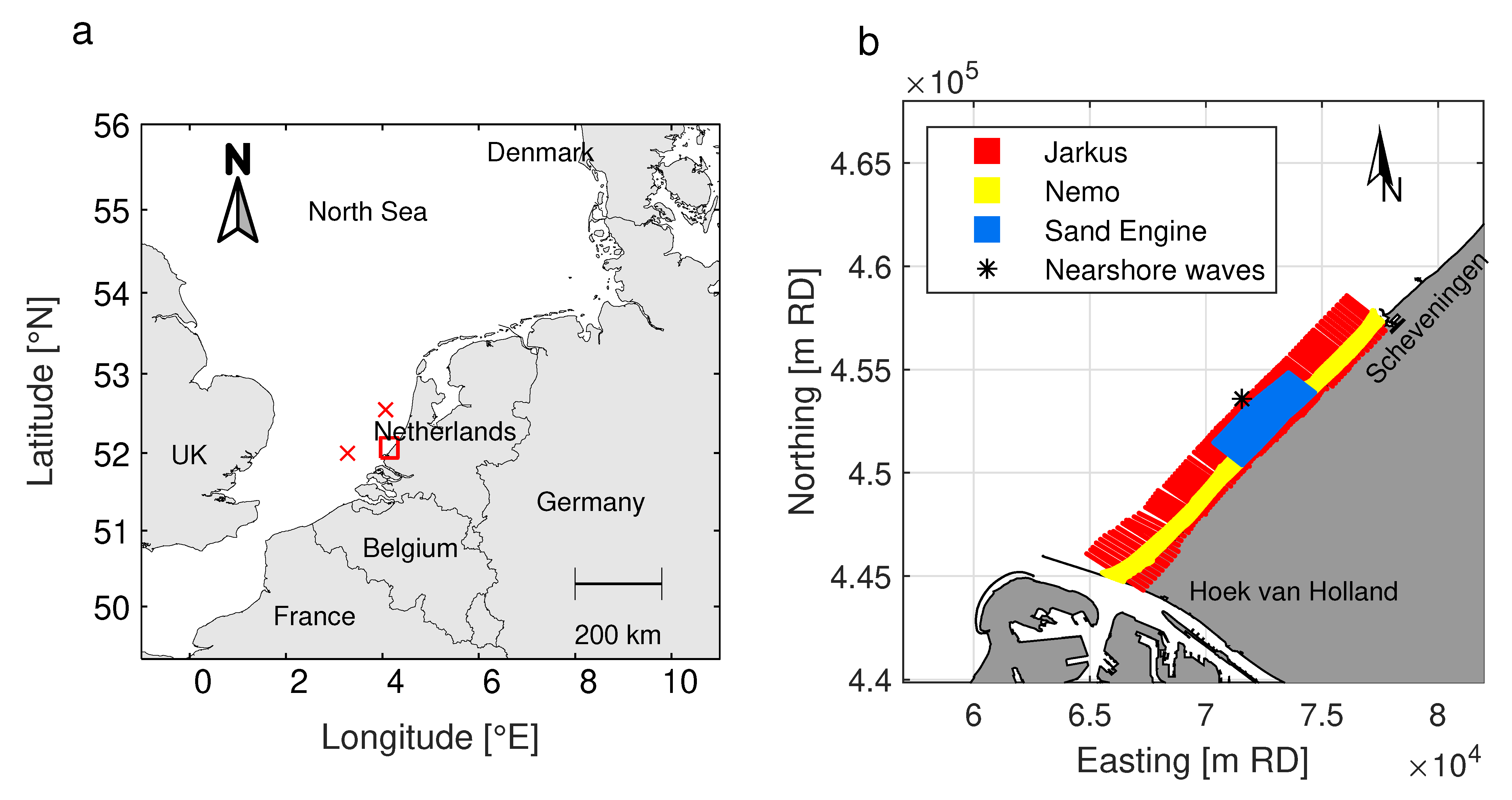
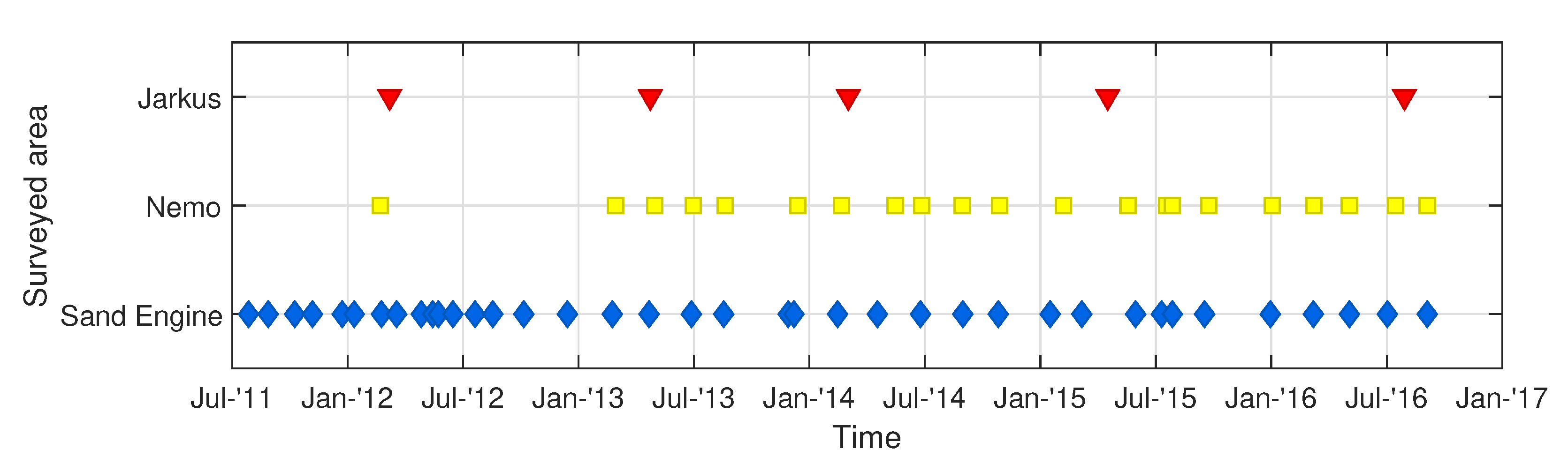
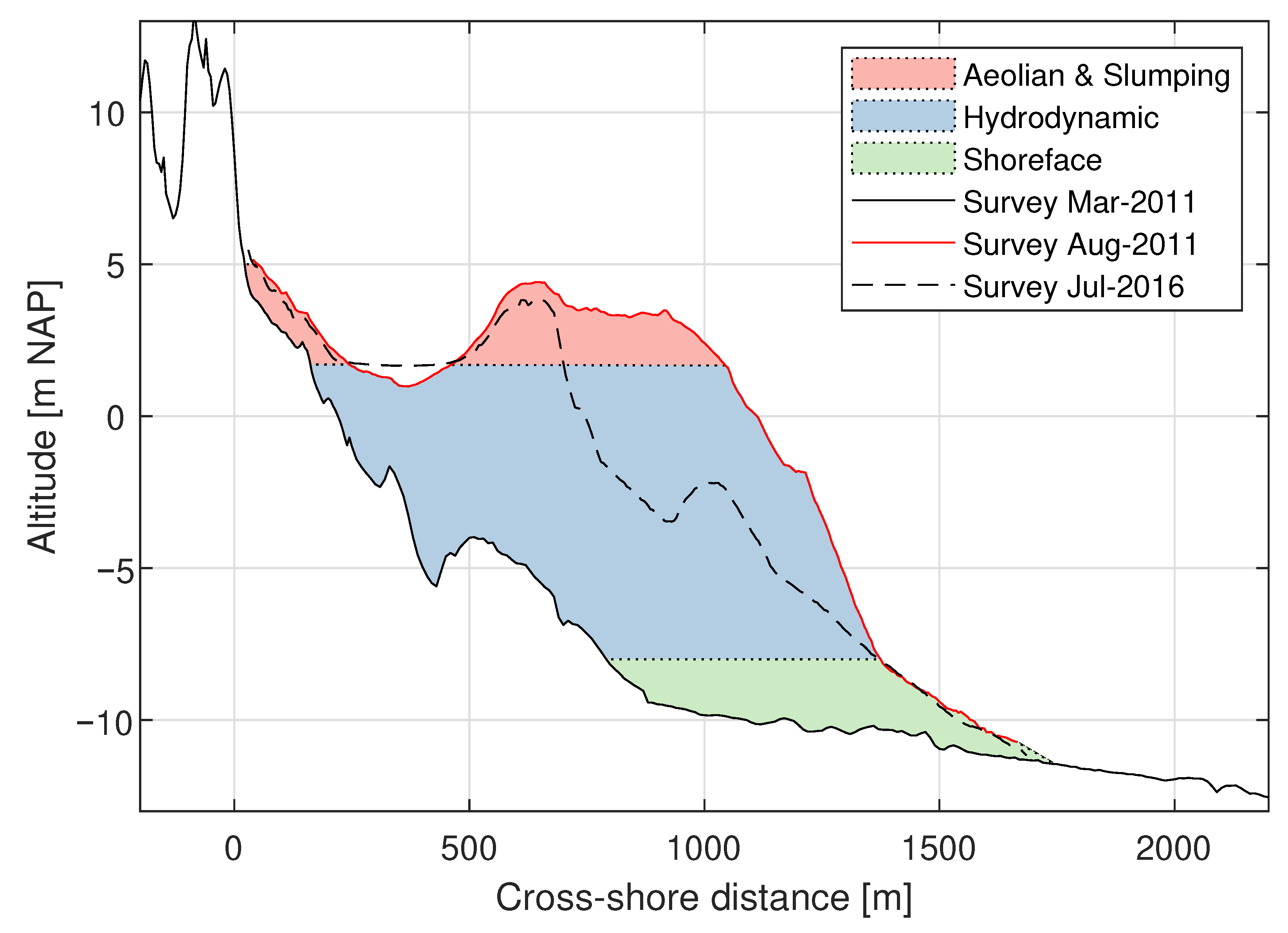
• The Sand Engine surveys [20] are collected during the Sand Engine project. Measurements in the Sand Engine domain (Figure 2b, blue area) are performed from August 2011 to September 2016 on a monthly time scale for the first year and approximately bi-monthly thereafter. The Sand Engine is surveyed in cross-shore transects with an approximate 40 m alongshore spacing. These transects reach from the dunefoot (around +5 m NAP) to the −8 m NAP depth contour offshore. Half of the transects reach further offshore all the way to the −11 m NAP contour. The surveyed area covers approximately 4.7 km alongshore and 1.6 km cross-shore.
• The Nemo surveys [21] are collected in the Nearshore Monitoring and Modelling: Inter-scale Coastal Behavior (Nemo) research programme. These data cover the remaining alongshore area of the Delfland coastal cell, both to the north and the south of the Sand Engine measurement domain (Figure 2b, yellow area). The first survey was performed in February 2012, and from March 2013, surveys are performed bi-monthly in conjunction with the Sand Engine surveys (Figure 3). Nemo surveys are surveyed in cross-shore transects with a 25 m spacing alongshore. The transects are shorter than around the Sand Engine, with a landward boundary at the dunefoot (+5 m NAP). The offshore boundary is situated round the −5 m NAP isobath in the southern part and −6 m NAP in the northern part. The surveyed areas cover 7.7 km (south) and 5 km (north) alongshore and about 600 m cross-shore. In this way the bulk of the littoral zone is covered in the measurements.
• The jarkus surveys [22] are part of the Dutch yearly coastal monitoring program (in Dutch: JAaRlijkse KUStmeting). The data cover the Delfland coast with an alongshore resolution of 250 m, from the land side of the dunes to approximately the −12 m NAP isobath. The jarkus surveys further cover the entire Dutch coast from the back of the dunes to at least 800 m offshore since 1965, e.g., [11,24].

The Sand Engine, Nemo and jarkus data sets are complementary in the spatial domain and provide a unique alongshore coverage of morphological measurements in the coastal cell (Figure 2b). Combining both the Sand Engine and Nemo data sets, a total 612 transects are measured alongshore, covering the entire coastal cell of 17.3 km with a bi-monthly temporal resolution. Time intervals between consecutive surveys of the Sand Engine and Nemo domain may deviate slightly between survey periods due to weather restrictions (Figure 3). The annual jarkus dataset provides a larger scale background for interpretation of the data.

Sand Engine and Nemo surveys are performed with a real-time kinematic differential global positioning system (RTK-DGPS) technique, using three different measuring vehicles. Land based surveying is performed with a 4WD quad bike, while water-based surveying is done using a jetski-equiped with single beam echosounder. Difficult terrains and shallow water are surveyed by a wheeled pole. All vehicles are equipped with RTK-DGPS, providing a vertical accuracy of 5 cm on land using the quad-bike, 3 cm for the wheeled pole and 10 cm for water-based measurements using the jetski [15,25]. The jarkus surveys in the considered time window are collected using lidar flights for the area above the low water line and ship based single-beam echo sounding in sub-tidal areas [11]. The reported vertical accuracy of these measurements is 15 cm for both techniques [26].

The raw $x,y,z$ point cloud data from the survey domains is combined and interpolated to the fixed set of cross-shore survey transects by bi-linear interpolation. Furthermore, a shore-normal orthogonal coordinate system was adopted with its origin at position (67067,444050) in the local Dutch Rijksdriehoeken coordinate system (EPSG:28992) and rotated 48.7 degrees clockwise. This results in 37 shore orthogonal altitude maps, 21 of which cover the entire Delfland coastal cell, including the Sand Engine area (blue and yellow area, Figure 2b), and 16 maps cover the Sand Engine area only (blue area, Figure 2b) [23].

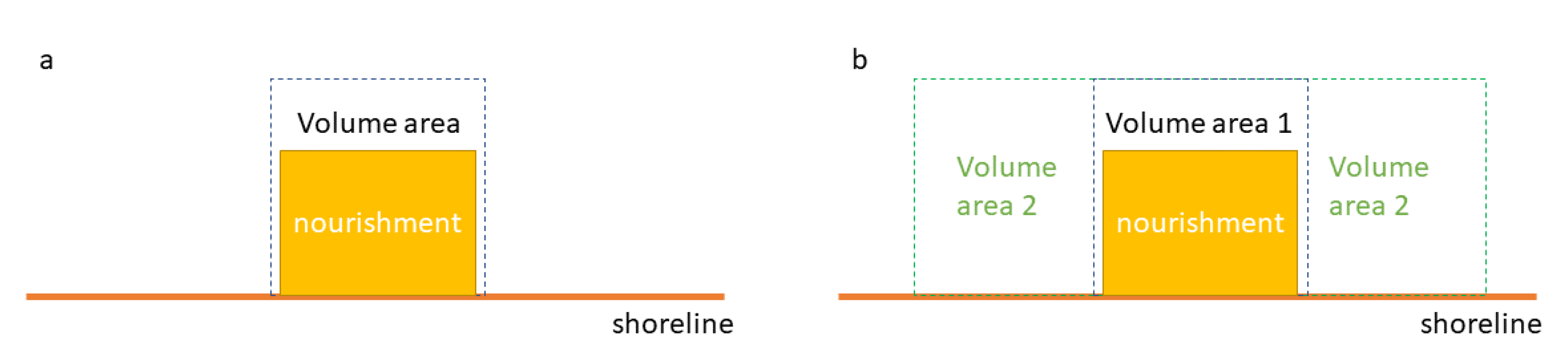
2.2. Volumetric Analysis

Quantification of the spreading of the Sand Engine peninsula is performed with a volumetric analysis on cross-shore transects. At all transect locations, the change in volume between every consecutive survey is determined. For each transect, independent time series are obtained consisting of either 21 (full coastal cell) or 37 (Sand Engine area) observations.

To maintain the large-scale overview, the coastal cell is divided in a few sediment budget areas representing different large-scale morphological behaviour (large erosive and accretive areas). Time-series of the volumetric development are obtained, by summation of the volumetric developments of the respective transects in these areas.

From the interpolated data, depth contours at different altitudes are derived to quantify planform shape development of the peninsula in time. Due to the presence of the lagoon and sub-tidal bars, depth contours may occur on multiple locations in the cross-shore profile. Therefore, the position of a depth contour in a transect is defined as the position of the most seaward crossing with the cross-shore profile.

Especially the alongshore extent of the peninsula is extremely difficult to determine in an accurate and foremost objective way. Therefore, a curve-fitting routine was applied on the depth contours. A Gaussian curve was adopted, due to its resemblance to the isobaths’ shape. The Gaussians’ parameters describe the macro features of the planform: alongshore extent, cross-shore extent and alongshore position of the planar centre of gravity. This approach is similar to De Schipper et al. [15] who applied this method for a shorter period of development. Fitting is done in shore orthogonal coordinates, using Equation (1).

$$y\left(x\right)=aexp\left[-{\left(\frac{x-b}{2c}\right)}^2\right]+d$$

(1)

In Equation (1), a is the cross-shore extent with respect to the isobath further alongshore, b is the alongshore position of the maximum cross-shore extent (mean), c is a measure for alongshore extent, and d is the cross-shore off-set from the reference line. The alongshore and cross-shore coordinates are given by x and y, respectively. The cross-shore extent of the nourishment’s isobath from the reference line is given by $a+d$, while the alongshore extent is defined here to be equal to $4\sqrt{2}c$. For an example of such curve-fit, see Figure 4.

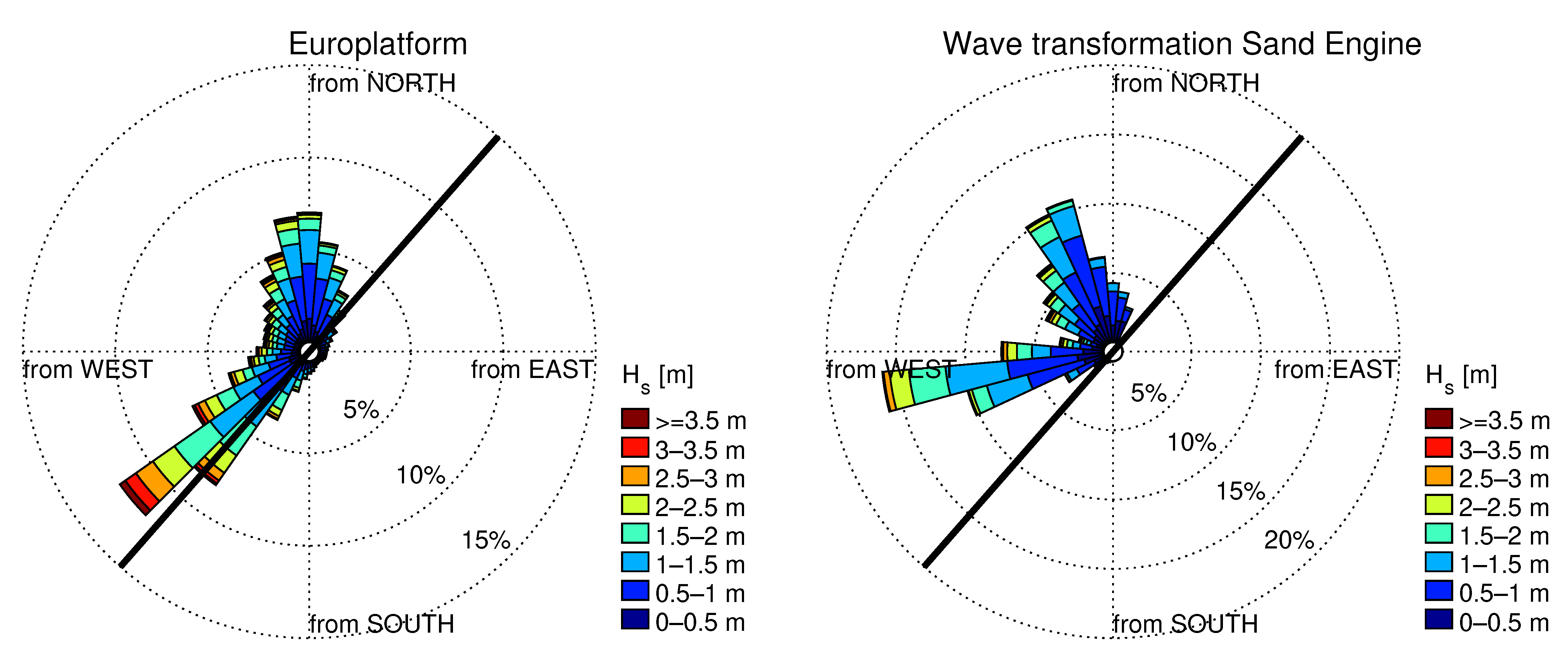
2.3. Wave Data and Transformation

The Holland coast is facing the relatively shallow North Sea and is therefore forced by a wave climate primarily consisting of wind waves. The mean significant wave height is around 1.3 m, and wave peak periods are usually around 5–6 s [27]. Two dominant sectors are present in the wave climate: waves approaching from the south-west and from the north. The south-westerly waves show a seasonal variability with higher waves from October to February, the northerly waves are more uniform throughout the year. However, during the most extreme storm events with an occurrence of less than once per year, waves usually come from the north-west. Such storms generate wave heights over 5 m, and wave peak periods around 9 s.

Along the Holland coast, waves are continuously measured at several wave stations, mostly located offshore. For this study these offshore wave parameters need to be transformed to nearshore conditions. Offshore wave parameters are obtained from the closest offshore wave stations: Europlatform and IJmuiden Munitiestortplaats. Both stations are located about 30 km offshore at 32 m water depth (Figure 2a). These time series of hourly wave conditions are subsequently transformed to nearshore (~10 m water depth) using the Holland Coast and Wadden (hcwd) wave transformation matrix [28]. This wave transformation matrix originates from previous extensive wave modelling using the Simulating Waves Nearshore (swan) spectral wave model [29]. The swan model was run using multi-decadal time-series from four offshore wave stations along the Holland and Wadden coast, which are then transformed to nearshore conditions resulting in the hcwd wave transformation matrix. For every grid-point in the transformation matrix, output can be generated provided that offshore wave time series are available in the desired time frame. Output of this wave transformation matrix has been validated against historical wave data from nearshore wave stations (1979–2001) [28], as well as a wave buoy near the Sand Engine (2011–2012). For this study, a single nearshore output location was chosen central in the coastal cell at about 10 m waterdepth. Nearshore wave data at the 10 m contour are further translated inshore using the dispersion relationship for linear water waves and Snell’s Law for straight and parallel depth contours. Breakpoint values are estimated at the water depth where the wave height exceeds 0.5 times the water depth. These are not including the curvature of the coastline due to the Sand Engine, and they provide a single estimate of H_b for the entire coastal stretch.

Figure 5 shows an overview of the offshore (left) and nearshore (right) wave climate. Towards the coast, significant wave height slightly decreases due to refraction and diffraction processes. Nearshore at 10 m water depth, the mean significant wave height is approximately 1.0 m. Wave direction near the Sand Engine also is more shore normal due to refraction. Storm significant wave heights are about 4 m, but more importantly, storms can generate significant surges along the coast, up to 2.2 m. These surges change the range of elevations at which the wave action has a morphological influence.

Nearshore wave series are analysed over the intervals between consecutive surveys. Several parameters were assessed, as suggested by Miller and Dean [30]: significant wave height, wave peak period, wave power (2), cross-shore wave energy flux (3), alongshore wave energy flux (4), Gourlay number (5) and Iribarren number (6). The cross and alongshore wave energy flux are the components of wave energy in their respective directions. The Gourlay or Dean number is a measure of wave steepness, scaled to sediment fall velocity [31,32]. The Iribarren number, or surf-similarity parameter determines the breaker type. All parameters are calculated for nearshore conditions at 10 m water depth, except for the Gourlay number, which is calculated for breaking wave conditions.

$$P=\frac{1}{16}\rho g{H}_s^2{c}_g$$

(2)

$$P_{cs}=Pcos\left(\theta -\alpha \right)$$

(3)

$$P_{ls}=Psin\left(\theta -\alpha \right)$$

(4)

$$\Omega =\frac{H_b}{w_s{T}_p}$$

(5)

$$\xi =\frac{tan\beta }{\sqrt{\frac{2\pi H_s}{g{T}_p^2}}}$$

(6)

In these equations P is the wave energy flux (wave power) [J/m], $H_s$ nearshore significant wave height [m], $c_g$ the wave group celerity [m/s], $\theta$ the wave from direction [deg N], $\alpha$ the shore-normal direction [deg N], $\Omega$ the Gourlay number [-], $H_b$ the breaking wave height [m], $w_s$ the sediment fall velocity in seawater [m/s], $T_p$ the peak wave period [s] and $\beta$ the cross-shore intertidal beach slope [m/m].

It is necessary to reduce the hourly wave data to match volumetric time-series. This is accomplished by first calculating the desired parameter (e.g., wave energy) and then taking an operation over the desired time-span (e.g., root mean square). Several operations were tested: minimum, maximum, mean and root mean square (rms). No spatial variation was applied to the hydrodynamic conditions at this stage.

Volume changes between consecutive surveys are examined to quantify the relation with variations in forcing on a monthly timescale. Time series of volume changes are linearly correlated to nearshore hydrodynamic parameters on a monthly timescale.

Profile volume changes are separated into net volume changes (Equation (7)) in the cross-shore profile and gross volume changes (Equation (8)):

$$\Delta V_{net}=\sum _{i=1}^n\left(z_{t,i}-z_{t-1,i}\right)·\Delta x·\Delta y$$

(7)

$$\Delta V_{gross}=\sum _{i=1}^n\left(\left|z_{t,i}-z_{t-1,i}\right|\right)·\Delta x·\Delta y$$

(8)

Net volume change is the sum of differences in bed level between consecutive beach profiles, subtracting local erosion from accretion. Gross volume change is the absolute sum of bed level change between consecutive profiles, adding local erosion and accretion. It is also a measure of cross-shore redistribution or profile adaptation. To filter out influences of local disturbances (e.g., bars and rip channels) volumes are aggregated over a 500 m alongshore moving window.

Besides wave driven currents, tidal and wind driven currents could enhance sediment transports. The alongshore flood current at the Holland coast is directed north-east and is slightly stronger than the ebb current, which flows to the south-west. Maximum spring-tide currents are 0.8 and 0.7 m/s respectively, resulting in a circa 0.1 m/s residual current in flood direction [12,27].

Simulations have shown that due to contraction of the tidal flow around the Sand Engine peninsula, bed shear stress is enhanced [33,34]. During the flood phase, tidal flow separation and eddy formation are observed at the Northern part of the Sand Engine peninsula, giving rise to enhanced particle dispersion [35]. Luijendijk et al. [33] attributed relative contributions of waves (75%), vertical tide (17%) to the magnitude of the eroded volume in the peninsula area during the first year. Other forcing mechanisms, such as tidal currents, surge and wind only modify—if omitted from the forcing—the initially eroded volume by 5% [33]. This shows that tidal currents have limited effect on large scale volumetric changes. Therefore, this paper will not examine specifically the role small variations in tidal forcing (e.g., timing of the neap-spring cycle) between consecutive surveys.

3. Results

The results of this study on the morphodynamics of the Sand Engine mega feeder nourishment are ordered from general observations to detailed analyses. First, the general planform adjustment is discussed; subsequently, the volume changes in the spatial and temporal domain are addressed. Then, a more detailed look into changes of the cross-shore profile is presented. Finally, the observed morphological changes are related to hydrodynamic forcing.

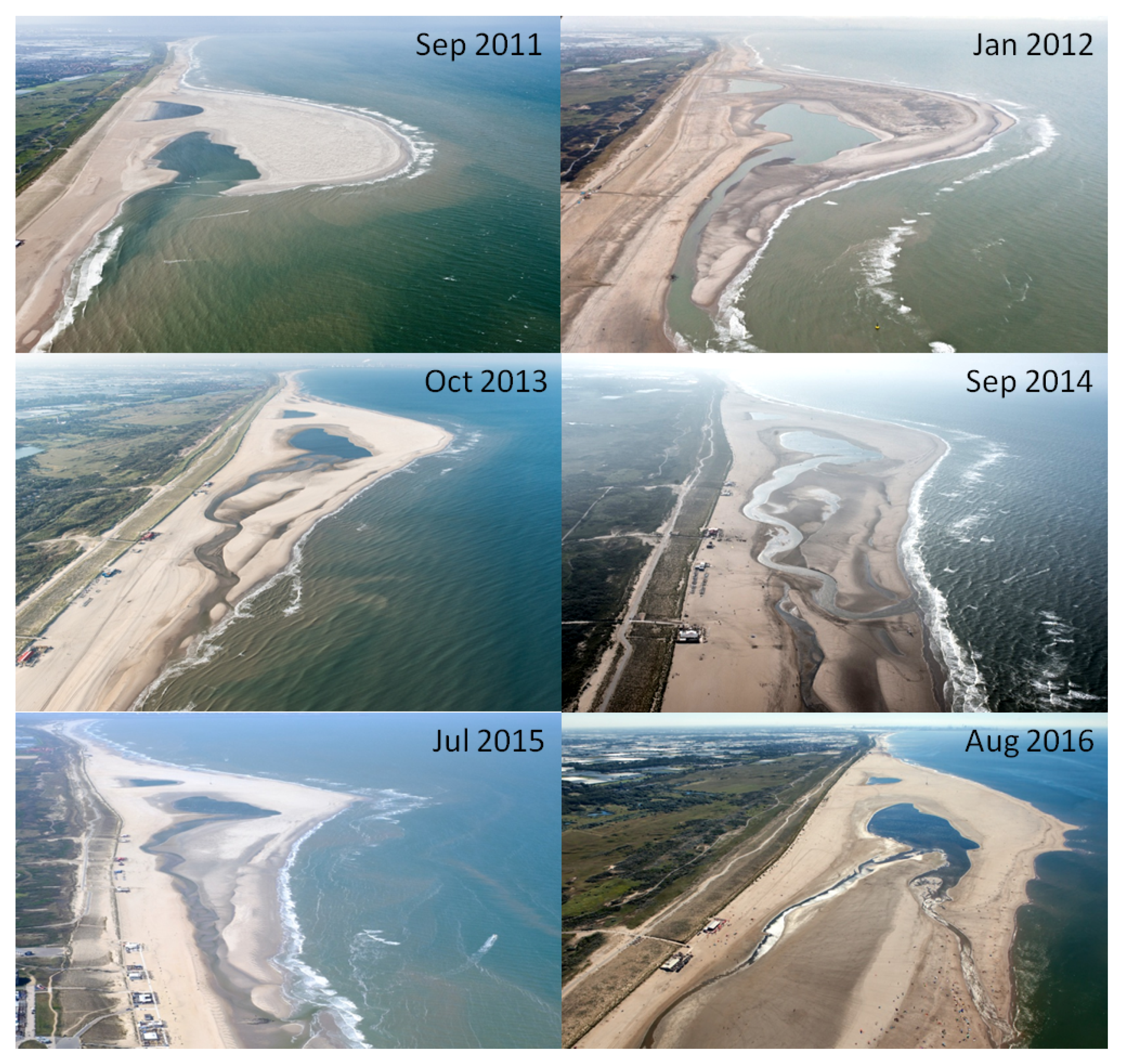
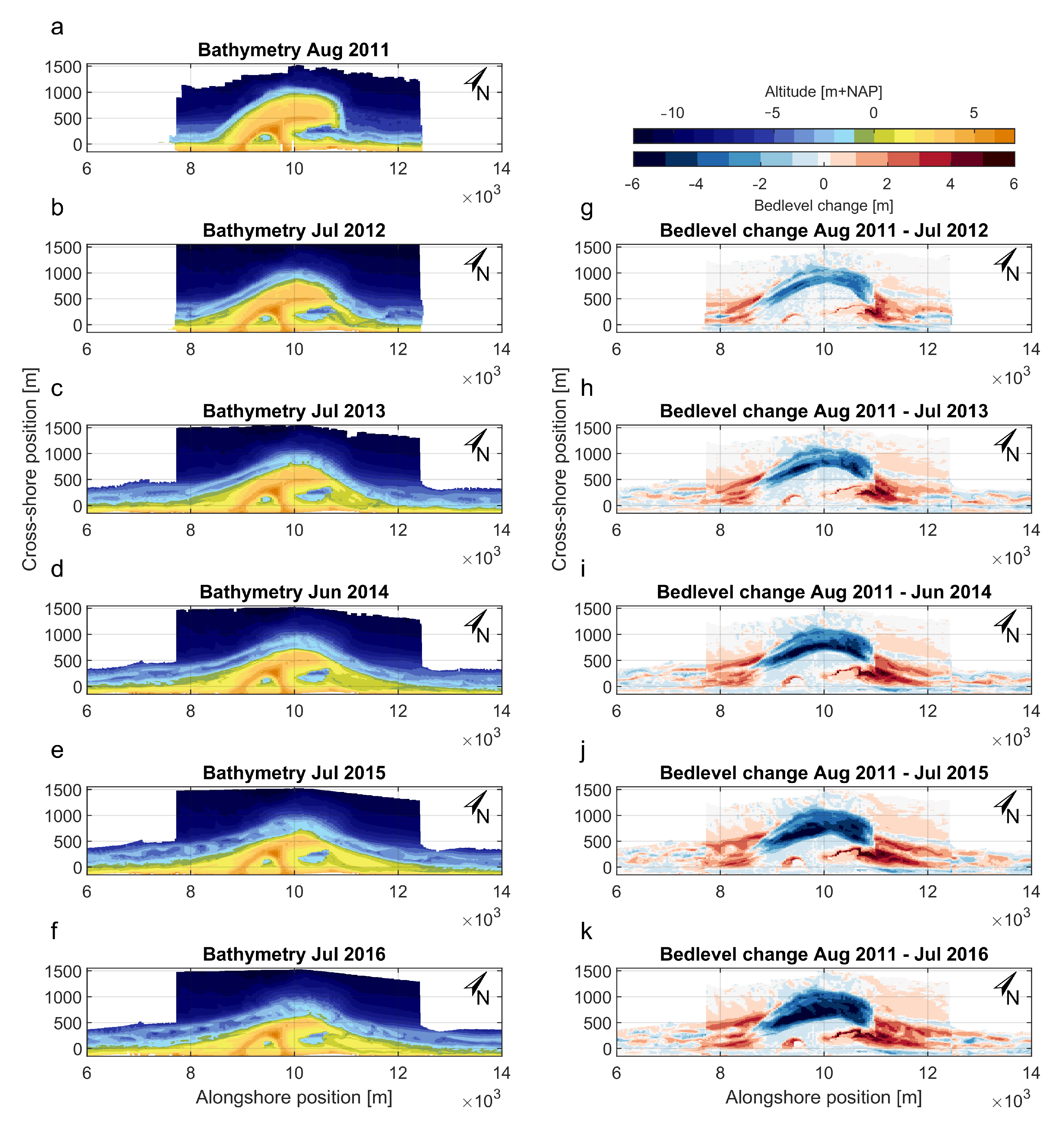
3.1. General Observations of Five Years of Sand Engine Development

The morphological changes of the Sand Engine peninsula and its immediate surroundings show significant zones of deposition on either side of the feeder nourishment (Figure 6). The Sand Engine peninsula was initially constructed as a hook-shaped peninsula, which was open to the north (Figure 6a). After a few months the opening to the lagoon began to close, only to remain connected through a tidal channel (Figure 6a,b). This tidal channel, which connects the lagoon to the sea, meanders and elongates along the beach towards the north. Throughout the survey period a new channel was formed twice, in December 2012 and January 2016 (Figure 6f). This channel created a shorter connection and became the main flow connection between the lagoon and the open sea. Over time these channels migrated to the north, eventually merging with the older channel. Although the old channels slowly silt up, their signature is still present in the beach morphology.

The main trend visible from these observations is erosion of the central part of the peninsula along its outer perimeter and deposition of sediments on both sides alongshore. The accretive areas extend in alongshore direction over time (Figure 6g–k). Locally the bed level change reaches 6 metres. The sub-aerial parts of the peninsula were eroded under aeolian influences while the lake and lagoon have captured part of this sand along their seaward perimeter (Figure 6g–k, [16]).

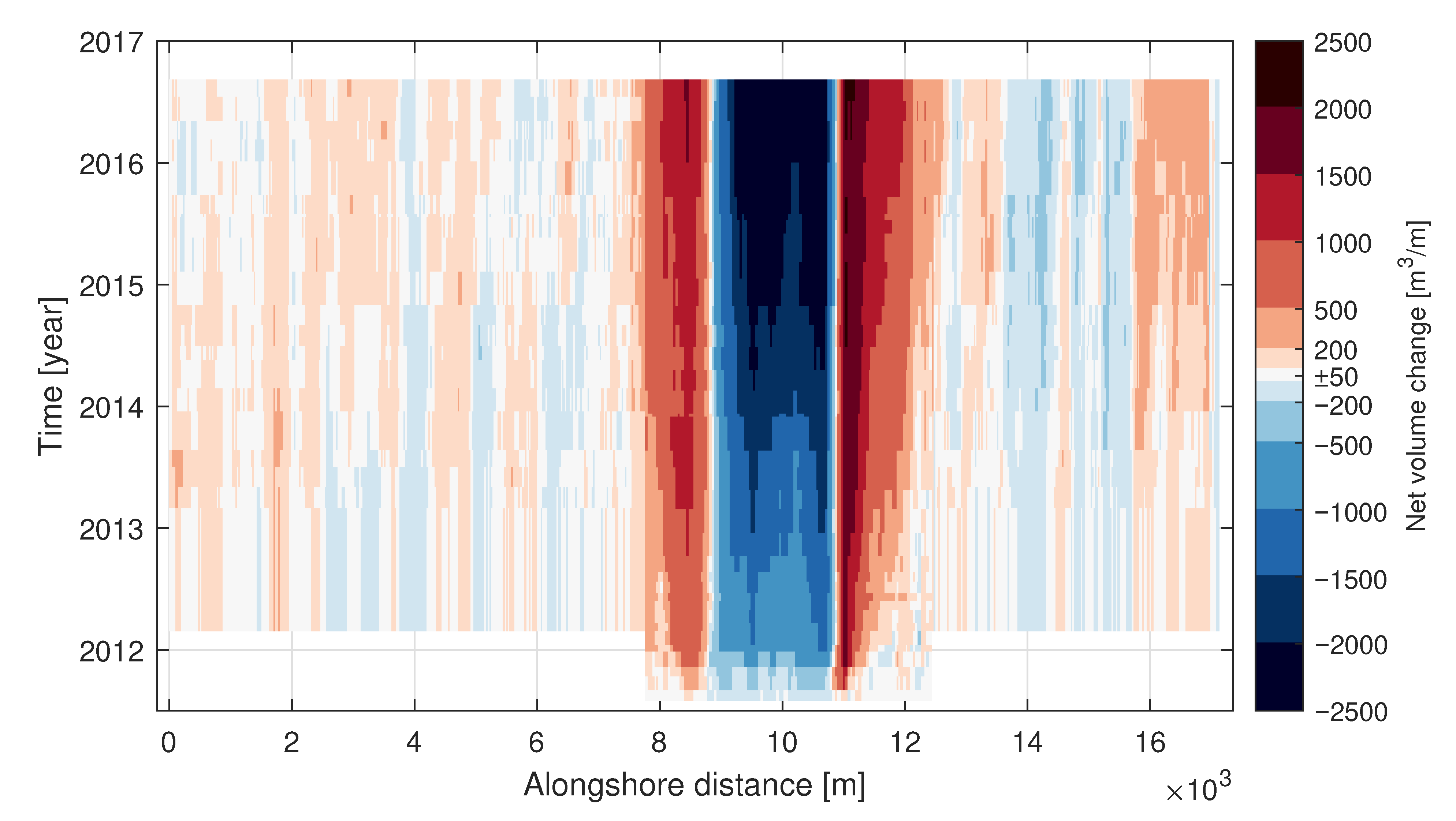
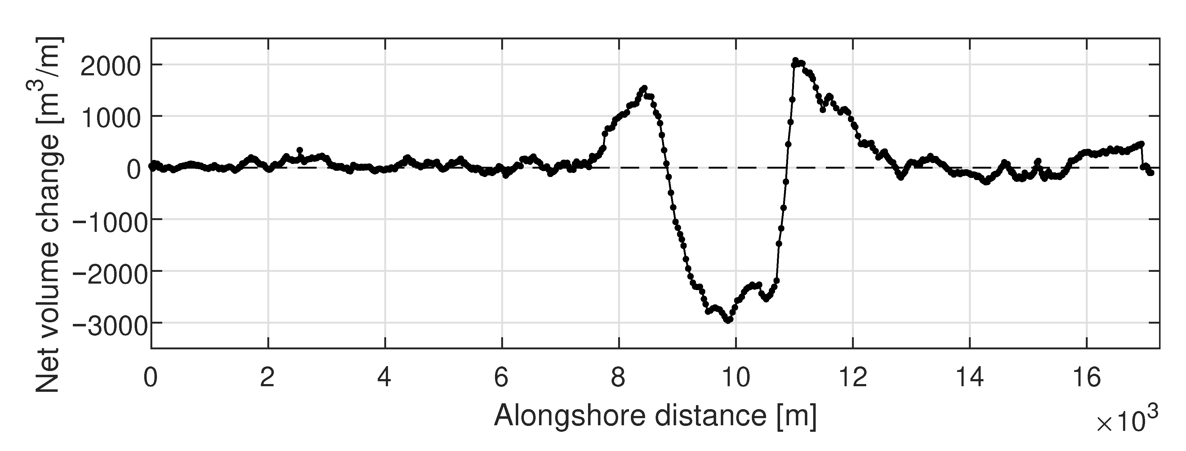
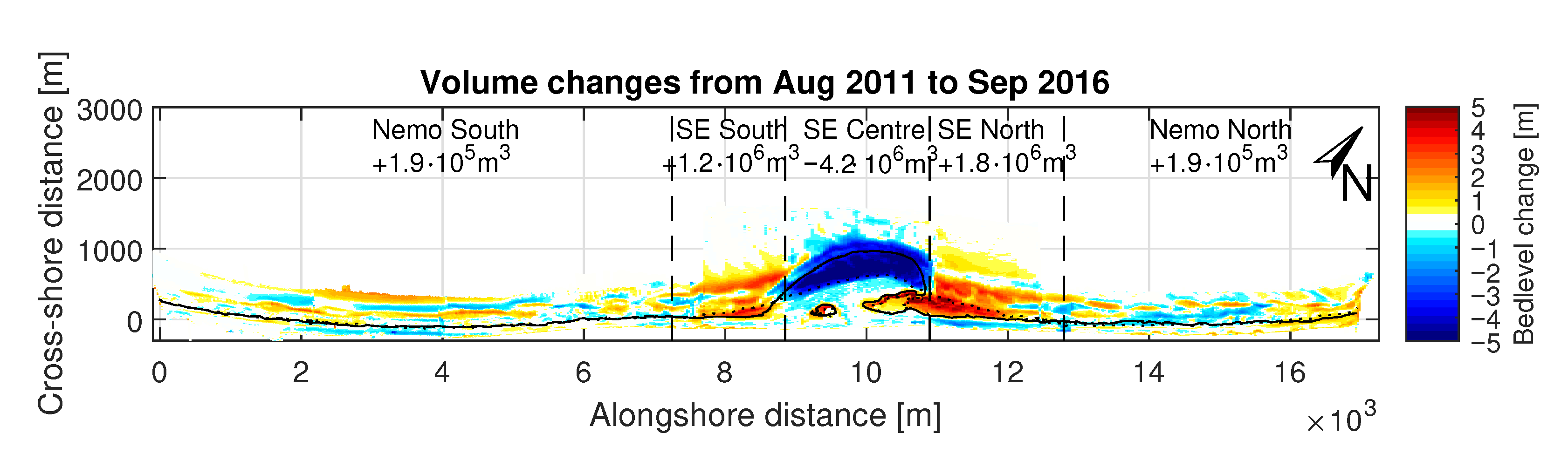
3.2. Volumetric Changes to the Nourishment and Adjacent Coastal Sections

Volumetric time series of all transects in the whole domain show the gradual alongshore spreading of the Sand Engine nourishment (Figure 7). Presented volumes are relative to the first survey. Accretive areas on both sides of the peninsula gradually extend alongshore in time during the 5 year period. In contrast, the erosive central area remains in place and the transitions from net accretion to net erosion remain in position on yearly time-scales. Most erosion occurs at a relatively confined area at the Sand Engine peninsula’s seaward perimeter throughout the years.

Net volume changes along the Delfland coast are dominated by local sediment dynamics (erosion and accretion) at and around the Sand Engine area. The erosion in the most seaward part of the peninsula shows a net volume loss in profiles up to 3000 m³/m, while the accretion at adjacent beaches reaches values of 2000 m³/m after five years (Figure 8). Further away from the nourishment, from approximately 3.5 km north and south of the Sand Engine peninsula centre, the net volume changes were smaller and typically up to ±150 m³/m or less. A distinct transition between this unperturbed coast and the region with large influence from the Sand Engine is clearly noticeable from Figure 8.

The coastal cell is divided in several sections alongshore to quantify the alongshore feeding of the local coastal profiles. Figure 9 shows the sediment budgets that are associated with the large scale sedimentation and erosion areas. Over the five years investigated, the central peninsula section eroded with a total of 4.2 × 10⁶ m³ (Figure 10a, green line). This is 25% of the original volume of the Sand Engine peninsula. The volume losses in the first year were more pronounced (1.7 × 10⁶ m³) than in subsequent years (0.6 × 10⁶ m³/y), and in the last years, the erosion is gradually decreasing. Accretion values on the adjacent coastal sections show a similar temporal pattern, with large initial changes and more gradual accretion in subsequent years (Figure 10a).

Deposition in the areas next to the Sand Engine amounts to 3.4 × 10⁶ m³. This deposition can be further specified to 1.8 × 10⁶ m³ just north, 1.2 × 10⁶ m³ just south and 0.4 × 10⁶ m³ further alongshore outside the most prominent area of sedimentation. Assuming conservation of sediment in the measurement area, ~20% of the distributed volume from the peninsula (0.8 × 10⁶ m³) could not be traced back in the survey area. There are several potential causes to which this loss can be attributed, for which no, or only partial proof can be provided, e.g., sediment that was blown into the dunes, ca. 0.25 × 10⁶ m³ [16], sediments transported offshore beyond the −12 m isobath and bed level lowering effects such as winnowing of fines and consolidation [15].

Monthly changes in volume were compared with nearshore monthly wave power and alongshore wave power (Figure 10c). The net alongshore wave power is directed towards the north during most of the year, as south-westerly waves prevail during most times. In a few quiet summer months, a small net flux towards the south can be observed (Figure 10b,c). Colours in panel b indicate the percentage of alongshore wave power to total wave power.

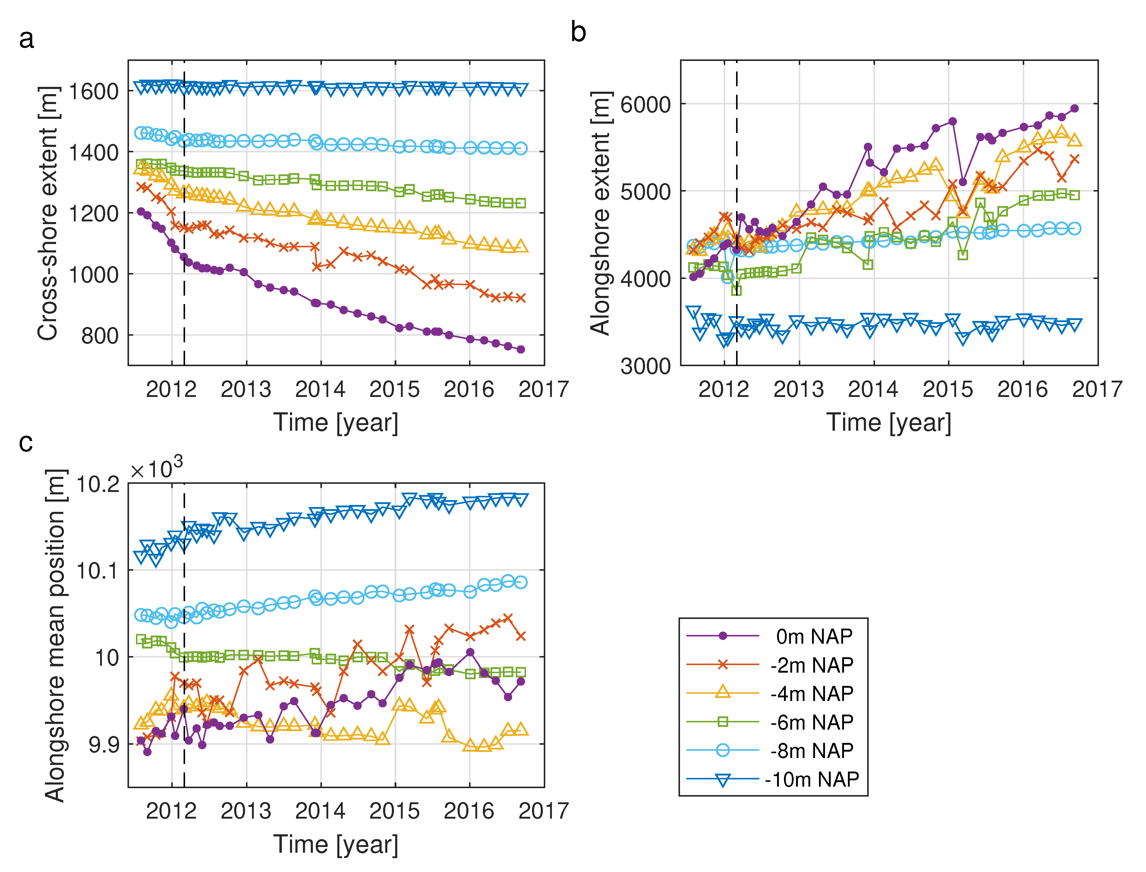
3.3. Sediment Spreading at Different Depths

The position and shape of the Sand Engine peninsula were analysed, based on its isobaths. Two different methods were employed: direct analysis and Gaussian curve-fitting (Equation (1)). It was revealed that the peninsula spreads differently on different altitudes (see Figure 11).

It must be noted that initially the 0, −2 and −4 m isobaths are not well characterised by the Gaussian curve, due to the blunt construction shape. Only after 6 months of diffusion (March 2012), reliable results for alongshore extent are obtained. At greater depths, the initial similarity is much better and the methods performs well immediately. Before March 2012, the alongshore extent is over-predicted, while cross-shore extent is under-predicted.

The point of maximum cross-shore extent, calculated with respect to the 0 m isobath prior to construction, shows a large retreat of several hundreds of meters (400 m) in the intertidal zone at 0 m NAP. The cross-shore set-back of the depth contours decreases with increasing water depth. At a level of −10 m NAP, no significant change in the cross-shore extent of the peninsula was observed in the five years (see Figure 11a, dark-blue line).

Similarly the alongshore extent varies with altitude (Figure 11b). Analogous to the change in cross-shore extent, the largest temporal changes in alongshore spreading were observed at the 0 m NAP level, and the response is decreasing over depth to a constant extent at an altitude of −10 m NAP. Initially the alongshore extent was largest around −8 m NAP since the 1:50 slopes at all sides of the peninsula cause a larger footprint at greater depths. As the higher elevations experience more spreading the maximum alongshore extent has shifted to higher elevations. In the intertidal zone (0 m NAP, Figure 11b purple line) the Sand Engine peninsula has spread alongshore to 5.8 km width in the five years. Initially spreading from 2.2 to about 4.5 km in the first half year while gaining a Gaussian shape.

The mean alongshore position of the peninsula, which is approximately at the point of maximum seaward extent, has not shifted significantly alongshore (Figure 11c). The translation alongshore is less than 100 m for all depth contours. This implies that diffusion of the peninsula is dominant over the alongshore advection of the peninsula. The slight northward advection also is not consistent over depth, with the −4 and −6 m NAP contours showing a small southward shift of the isobath centre of mass (Figure 11c, yellow and green lines).

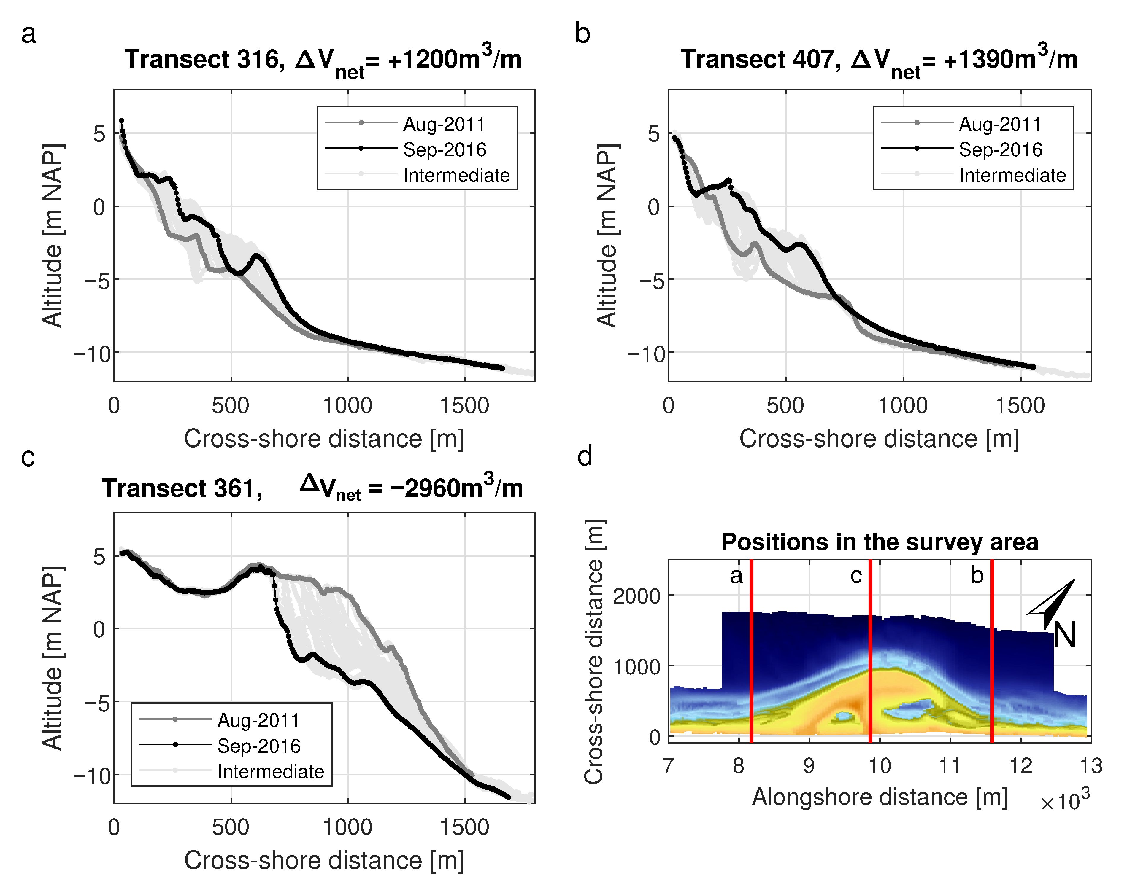
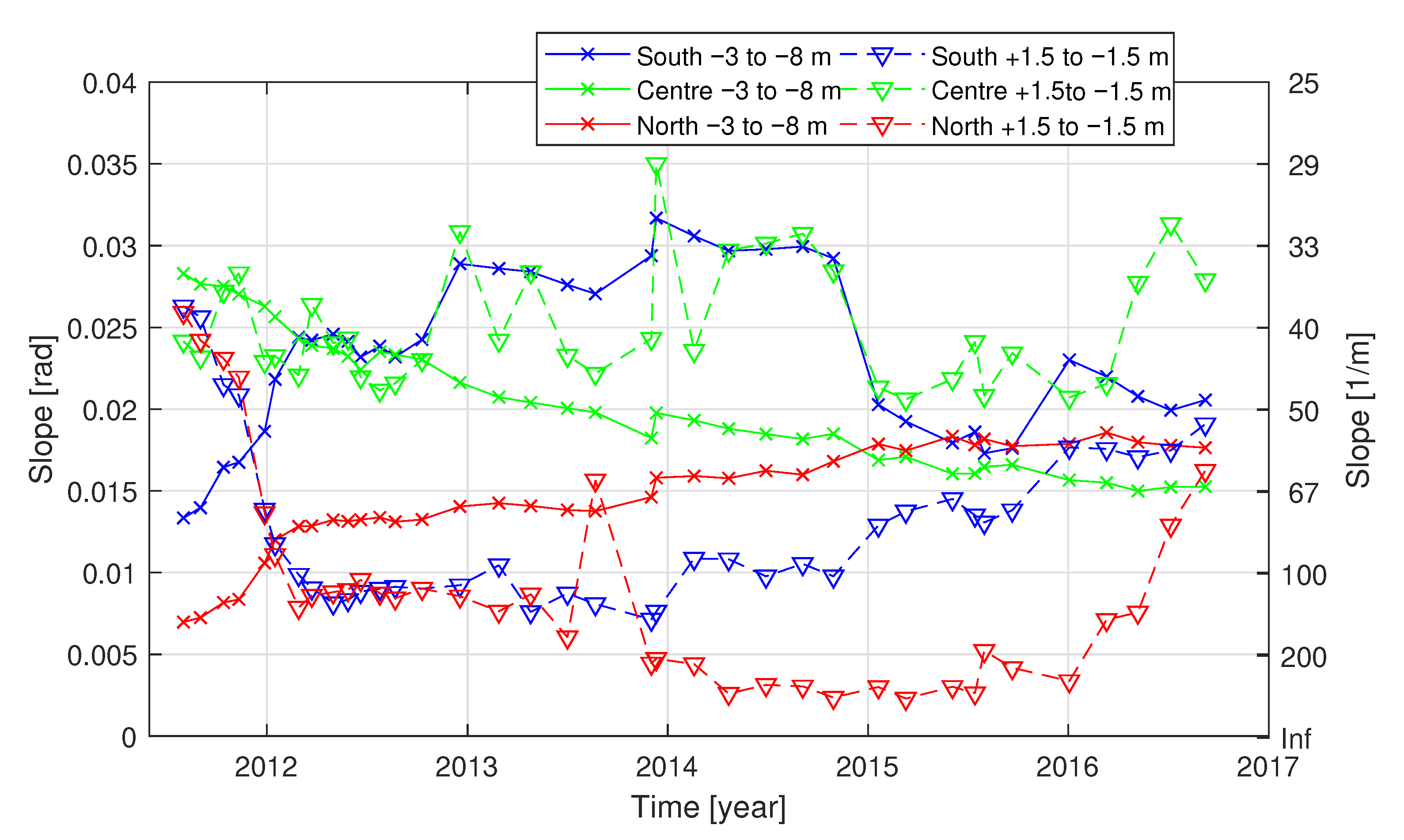
3.4. Development of Cross-Shore Profile Shape

The depth dependent evolution of the depth contour lines indicates that cross-shore profile shape is adapting on the timescales of years. Figure 12 shows the profile development of selected typical erosive and accretive profiles.

Cross-shore profile slope was derived for the morphological active depth range. The lower limit is at the depth of closure, while the upper limit is determined by wave run-up, or slumping at the eroding peninsula section. As shown in Figure 12c the central peninsula’s profile changed from convex to concave in five years. Therefore two ranges are assessed individually: lower profile, here defined as −3 m to −8 m NAP and upper profile, here defined as +1.5 m to −2 m NAP. The alongshore averaged slope of the lower profile (−3 m to −8 m NAP) in the coastal cell is ~1/85. The lower slope of erosive profiles becomes milder over time, as erosion decreased from the intertidal zone downward.

Here, alongshore averaged results are shown from three morphologically distinct sections along the peninsula: South located at 8−8.7 km alongshore, Centre at 9.3–10.6 km and North at 11–11.8 km alongshore. This gradient changes the lower slope from 1/35 to 1/67 along the central peninsula section. Meanwhile, the upper profile varies between 1/30 and 1/50 over time (Figure 13). The accreting South and North sections are situated largely outside the peninsula’s initial footprint. These areas show a rapid increase of lower profile slope together with a rapid decrease of upper profile slope in the first half year. The southern area’s shoreface steepened up to 1/33 but has reduced to 1/50 since 2015. The upper profile slope initially decreased to 1/110, but is increasing again since 2014. The northern spit exhibits a more gradual increase in lower profile slope; its slope in the upper profile rapidly changed to 1/120 in 6 months (Figure 13).

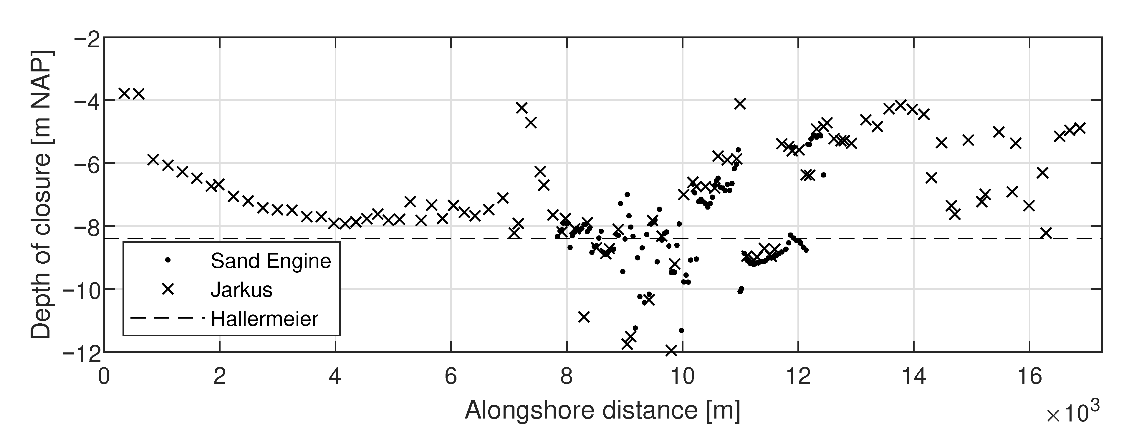
3.5. Depth of Closure

The depth of closure (DOC) in the coastal cell is examined to evaluate how the depth of closure estimates compare to the observed extend of morphological activity along the peninsula. It is defined as the altitude in the cross-shore profile below which no significant morphological changes are present.

When sufficient bathymetry surveys are available in a location, the depth of closure can be determined from statistics of bed-level variability. By setting a threshold on the standard deviation of the bed-level of 0.20 m, the most offshore location with significant change is determined. The depth of closure has been identified for all transects, using statistics of the bed-level. Using the jarkus surveys from 2012–2016, this results in a derived depth of closure between −5 and −10 m NAP, depending on the location in the coastal cell (Figure 14). Comparison to the closure depth calculated from 37 Sand Engine surveys shows good agreement.

Harbour moles are present at alongshore positions 0 and 17.2 km, which influence the local morphology and nearshore hydrodynamics. In the southern section from 0 to 7.5 km alongshore the depth of closure slowly increases to −8 m NAP over the first 4 km. At the Sand Engine Section (7.5–12.5 km), the closure depth stays around −8 m until the tip of the peninsula at 10 km, then decreasing to −4 m NAP near km 14. Morphodynamic activity associated with bars is lower here than in other parts of the coastal cell, so the most offshore bar does not trigger the DOC criterion. In the northernmost part, the closure depth varies between −5 and −7.5 m NAP. Migrating local features (e.g., mega ripples) on the sea-bed may just trigger the depth of closure criterion, resulting in a DOC below −10 m NAP. This explains most of the variability in Figure 14. The sudden change in depth of closure between 11 and 12 km is associated with deposition just north of the peninsula.

Secondly a general check is performed using the Hallermeier [36] equation in the form of Hinton and Nicholls [19] (Equation (9)), which is based on wave-statistics.

$$d_{DOC}=2.28H_{s,e,t}-68.5\frac{H_{s,e,t}^2}{g{T}_{e,t}^2}$$

(9)

In this equation, the depth of closure $d_{DOC}$ is referenced to mean low water level (i.e., −0.68 m NAP), $H_{s,e,t}$ is the nearshore significant wave height exceeded 12 hours per t years, and $T_{e,t}$ is the associated peak wave period in seconds. Comparing to Hallermeier [36], based on the transformed wave data in the five years considered, the annual depth of closure is at ~−7.8 m NAP and the five years value is −8.4 m NAP. This is in line with the values from the statistical method and values presented in Hinton and Nicholls [19].

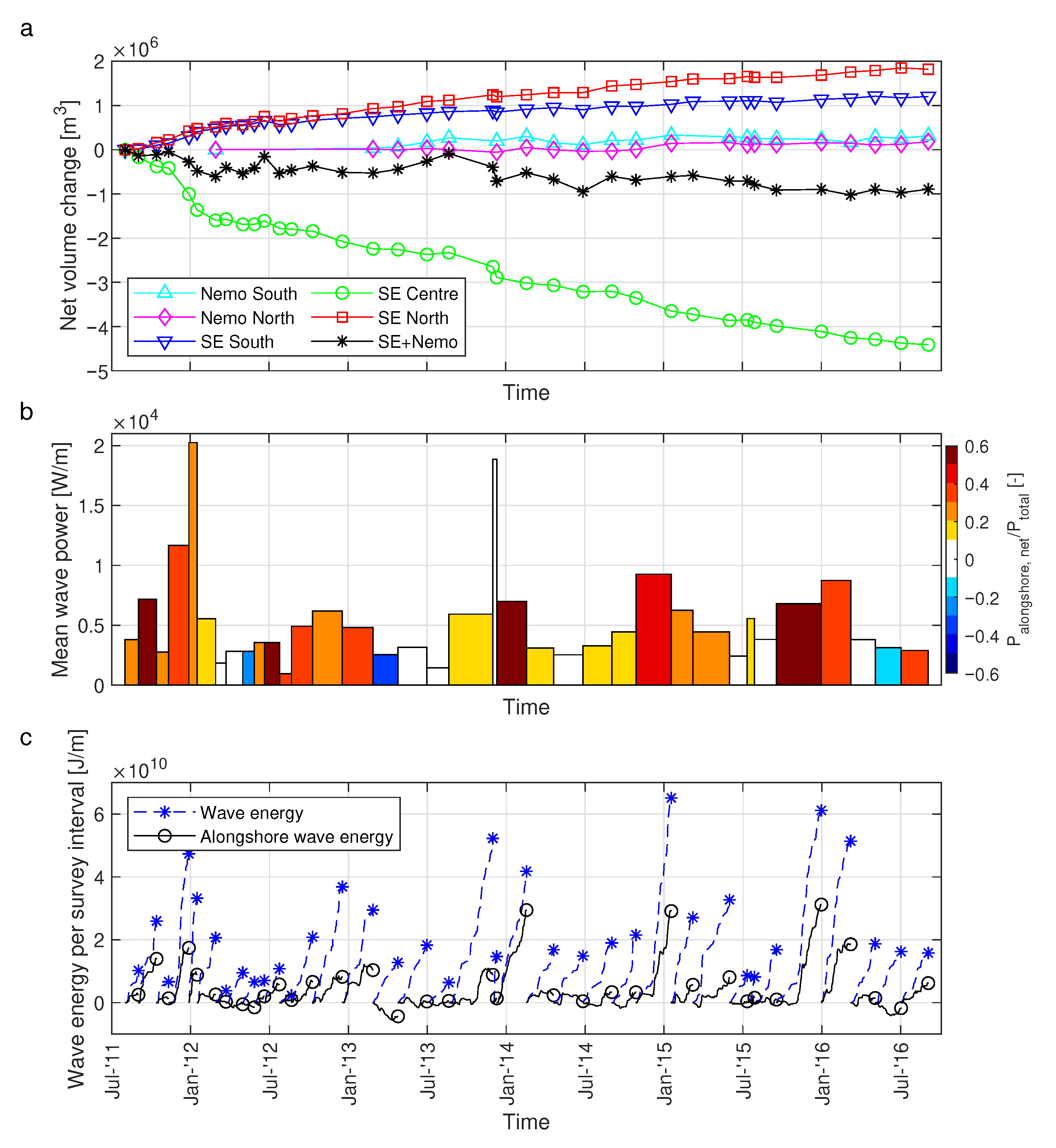
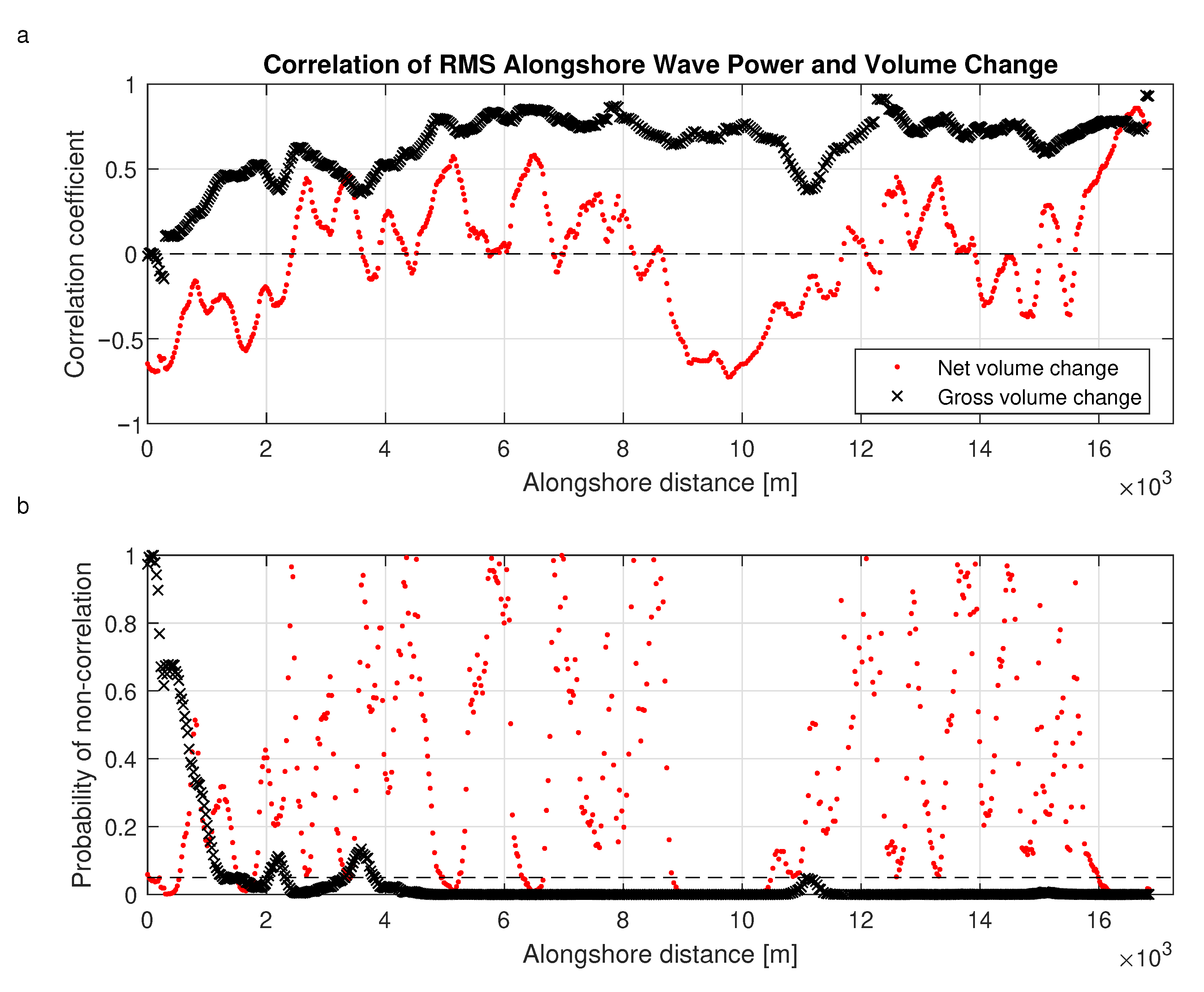
3.6. Cross- and Alongshore Response to Changing Forcing Conditions

Volume changes between consecutive surveys are examined to quantify the relation with variations in forcing on a monthly timescale. Both gross (Equation (8)) and net volume changes (Equation (7)) are assessed. Non-zero net cross-shore volume changes are indicative of alongshore redistribution of sediment from one profile to another. Gross volume changes on the other hand also map sediment redistribution within the profile.

Good correlations are found between forcing and volume changes at the eroding section of the Sand Engine peninsula. Both net and gross volume changes are significantly correlated to several of the hydrodynamic parameters with high correlation coefficients. However, there is no large difference between the parameters, with respect to the correlation coefficients, as shown in

Table 2. Correlation coefficients of volume change and hydrodynamics at the Sand Engine’s centre. The best correlation per column is presented in bold. Correlations with probability of non-correlation >0.05 are striked.

	Gross Volume Change				Net Volume Change
Parameter	Min	Mean	Max	Rms	Min	Mean	Max	Rms
Hs	0.13	0.70	0.69	0.72	$-\cancel{0.12}$	−0.65	−0.74	−0.68
Tp	$\cancel{0.27}$	0.51	0.57	0.55	$-\cancel{0.21}$	$-\cancel{0.43}$	−0.54	−0.47
P	$\cancel{0.23}$	0.64	0.68	0.63	$-\cancel{0.20}$	−0.59	−0.74	−0.61
Pcs	−0.54	0.59	0.69	0.58	0.59	−0.56	−0.77	−0.59
Pls	−0.78	−0.61	0.37	0.76	0.75	0.52	−0.51	−0.65
|Pls|	$\cancel{0.25}$	0.74	0.76	0.76	$-\cancel{0.22}$	−0.63	−0.75	−0.65
$\Omega$	$\cancel{0.13}$	0.69	0.73	0.72	$-\cancel{0.13}$	−0.65	−0.61	−0.69
Frsurf	−0.72	$-\cancel{0.34}$	$\cancel{0.44}$	$\cancel{0.04}$	0.72	$\cancel{0.32}$	$-\cancel{0.39}$	$\cancel{0.01}$
$\xi$	$-\cancel{0.46}$	$-\cancel{0.35}$	$\cancel{0.40}$	$-\cancel{0.29}$	$\cancel{0.46}$	$\cancel{0.38}$	$-\cancel{0.34}$	$\cancel{0.33}$

. For this specific part of the coast, rms wave height or alongshore wave energy flux appear to correlate the best, while for correlation with net volume change cross-shore wave power appears to correlate well too. Note that alongshore wave power is generally negative due to dominant waves from South of shore-normal, further net volume change at the Sand Engine’s centre is negative due to continuous erosion, occasionally leading to negative correlation coefficients.

To widen the scope of correlations, spatial differences in the coastal cell are addressed. Figure 15 shows an example of the alongshore variation in correlation coefficients for the rms wave energy. Correlations with gross volume changes are significant in most of the coastal cell (Figure 15, black crosses). Contrastingly, correlations with net volume change only show significant correlations at the central (eroding) section of the peninsula (8.8–10.3 km) and at a few small sections in the coastal cell (Figure 15, red dots).

4. Discussion

4.1. Differences in Behaviour in the First Year Compared to Following Years

Morphological changes in the first year after construction are significantly higher than in any of the subsequent years (Figure 10a). This is in line with observations of De Schipper et al. [37] and Elko and Wang [9], who suggest that large initial changes may be caused by the steeper man-made cross-shore profile. Indeed, slopes of the Sand Engine peninsula were steeper just after construction and the cross-shore slope of the eroding part is becoming milder in time. Further differences may be caused by the stronger coastline curvature, which greatly reduces in the first half year after construction.

Initial modelling attempts and observations of the first year indicated rapid change of the Sand Engine planform shape [2,15,17]. Furthermore, long-term modelling indicated, beside some alongshore spreading, strong advection of the nourishment towards the north [2,17]. However the observations presented here show no evidence of alongshore advection of the nourishment in the 5 year period. Instead, mainly diffusion of the nourishment is observed, which is also simulated by improved modelling by Luijendijk et al. [33] and Arriaga et al. [38].

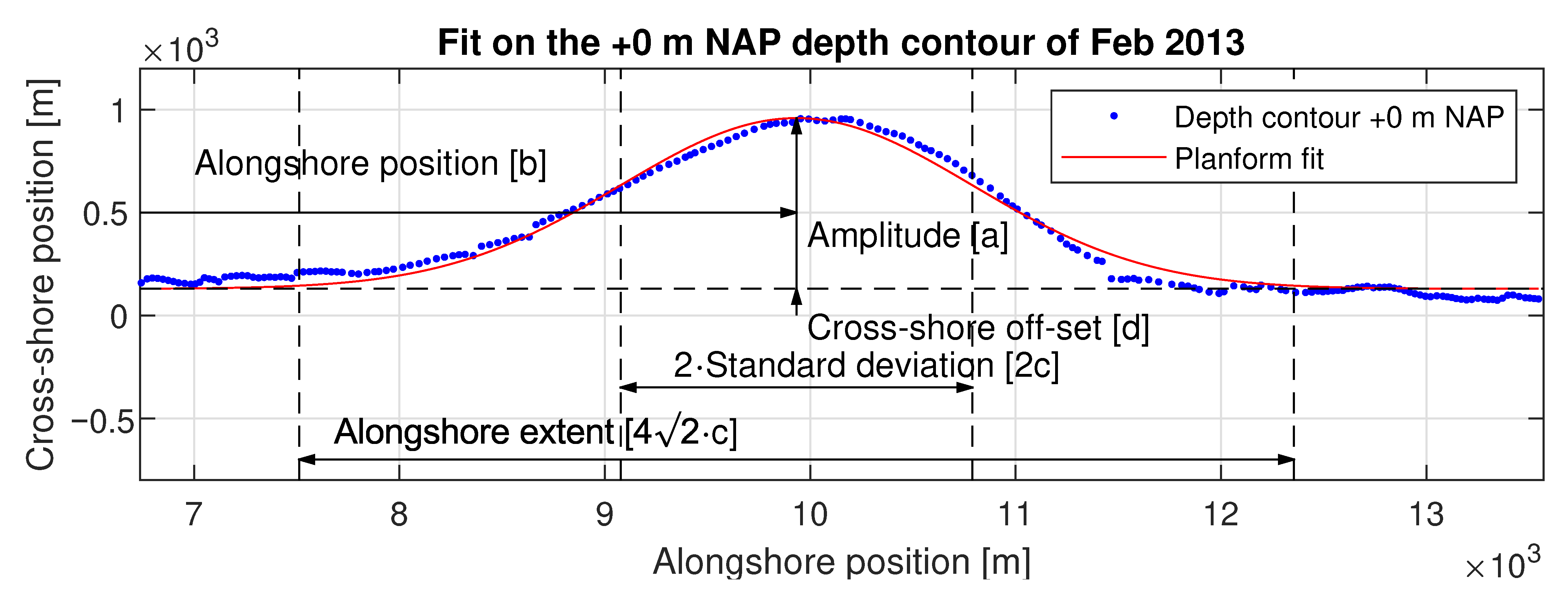
4.2. Detection of Planform Parameters

Plan form adaptation of the Sand Engine peninsula were tracked in time at different altitudes and summarised in three parameters: cross-shore extent, alongshore extent and alongshore position of the planar centre of gravity. Cross-shore extent and alongshore position can be easily detected directly from the bathymetry. However, an objective measure of the alongshore extent of the nourishment is harder to obtain. Initially the peninsula’s planform attaches sharply to the pre-nourishment isobaths, but due to the diffusional behaviour, this boundary becomes increasingly hard to determine. Fitting of Equation (1) to isobath coordinates is therefore a suitable method that produces objective parameters describing the planform development at different altitudes.

However, due to the blunt initial planform shape of the peninsula, depth contours between 0 and −4 m NAP do not fit particularly well to a Gaussian shape in the first six months after construction (before March 2012, indicated in Figure 11). This causes an over-estimation of the cross-shore and alongshore extent. At greater depths the initial similarity is much better. After six months, the planform of all depth contours fits to a Gaussian shape with a root-mean-square error of less than 60 m.

4.3. Cross- and Alongshore Response to Changing Forcing Conditions

Gross volume changes (Equation (8)) correlate well to spatially aggregated wave power proxies. A high probability of correlation and little alongshore variability in correlation coefficients are found along the coastal cell, except for the area near Hoek van Holland (Figure 15a). This could be expected, since energetic waves stir up much sediment and are able to transport it, resulting in relative large changes in profile shape. The relatively low correlations found near Hoek van Holland can be attributed to wave shadowing by the large harbour moles, which is not captured in the single wave power time series applied to the coastal cell.

Net volume changes (Equation (7)), correlate well around the eroding part of the Sand Engine peninsula and near the boundaries of the survey domain. This implies that larger erosion from the peninsula is driven by larger energetic wave conditions. At the same time, no significant correlation between wave power and the amount of accretion is found at the adjacent accretion areas (Figure 15b). It is generally known that the most energetic wave events stir up the most sediment and cause erosion and potential large alongshore feeding. The spatial characteristics of this alongshore feeding are likely dependent on relative angle of wave incidence. This dependency might influence the correlation between local wave power and accretion in a negative way at accreting areas. Furthermore, alongshore spreading of the sediment and associated changes in coastline orientation cause the local sedimentation rate to change in time.

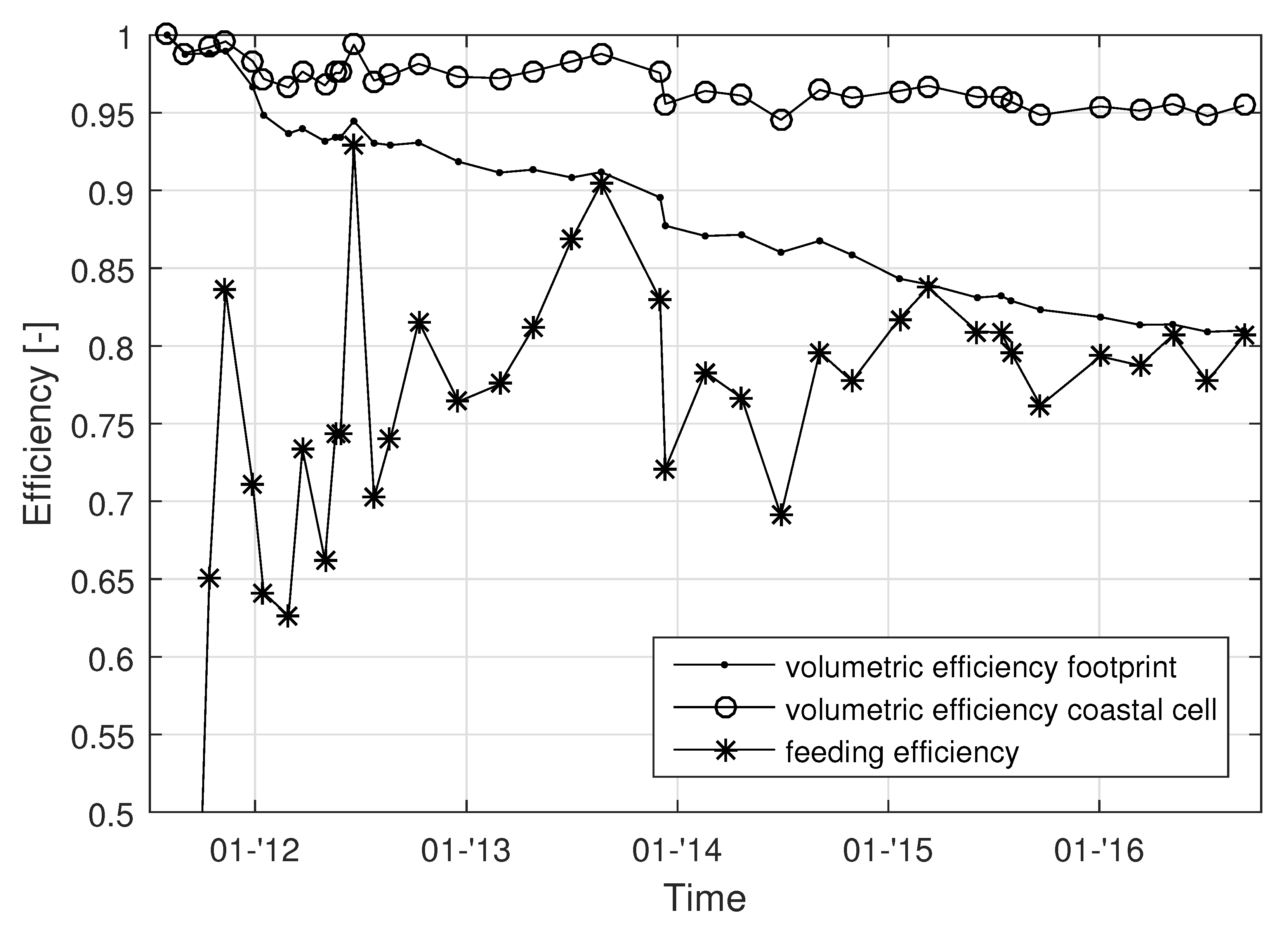
4.4. Efficiency of Nourishments

In a local approach, the efficiency $\eta$ of a nourishment is traditionally calculated as the volume of sand remaining within the initially nourished boundaries after certain time [3,4,39]; see Figure 16a.

$$\eta =1-\frac{\Delta V_{\mathrm{net}}}{V_{\mathrm{Nourishment}}}$$

(10)

where $\Delta V_{\mathrm{net}}$ is the change in sediment volume at the nourished site over time, and $V_{\mathrm{Nourishment}}$ is the original sediment volume used for the project. For a mega feeder nourishment however, the sand is intended to disperse over the coastal cell, demanding an analysis on a larger scale. To discuss the efficiency of a mega feeder nourishment the sediment redistribution is also of interest, in addition to the remaining volume. Therefore, we propose a feeder efficiency parameter ${\eta }_{\mathrm{feed}}$. This efficiency parameter describes how much of the loss from the feeder nourishment in the central part of the project area is compensated for by accretion on adjacent shorelines:

$${\eta }_{\mathrm{feed}}=\frac{\Delta V_{\mathrm{Adjacent}}}{-\Delta V_{\mathrm{Nourishment}}}$$

(11)

where $\Delta V_{\mathrm{Adjacent}}$ and $\Delta V_{\mathrm{Nourishment}}$ represent the change in volumes in adjacent coastal section and the feeder nourishment respectively. See Figure 16b. The feeder efficiency provides a simple quantitative parameter for the assessment feeding in the alongshore area. For the Sand Engine pilot experiment ${\eta }_{\mathrm{feed}}$ is approximately 0.8, indicating that at least 80% of the eroded sediments from the peninsula are compensated by accretion elsewhere in the survey domain.

To compare both definitions, time series of both the local efficiency and the feeding efficiency are presented in Figure 17. After five years, 95% of the nourished volume (17.5 × 10⁶ m³) is still present in the survey domain, while only 80% is present in the footprint area of the initial peninsula. The feeder efficiency appears to be low initially, then increasing and stabilising to ~80% after three years. Low feeder efficiency values in the early stages are assumed to originate mostly from measurement inaccuracies related to relatively small volume changes.

Considering the trends in the development of the nourishment volume, it is unclear if the nourished volume of the Sand Engine will be fully spread over the coastal cell, nor from the nearshore zone after the expected 20 years of the foreseen lifetime. From Figure 7 and Figure 11b the change in alongshore extent over the first five years is shown to be 0–400 m/year, depending on the elevation. Furthermore, it is shown that the rate of spreading is decreasing in time, thus the whole 17 km coastal cell might not be covered in the next 15 years. The observed sedimentation and erosion patterns further suggest that most of the sediment is deposited in the nearshore zone, above the depth of closure and below the high water mark.

4.5. Considerations for Future Designs

Limited bed-level changes are found below −8 m NAP (Figure 12 and Figure 18). Therefore, no clear evidence is found that the Sand Engine significantly influences the morphological processes on the deeper shoreface on the time scales of $\mathcal{O}$ (5 years). Although sediment transport may ultimately change these low parts of the feeder nourishment, the associated time scales of the development may be very long.

At the Sand Engine, approximately 15% (2.6 × 10⁶ m³) of the nourished sand is placed below the −8 m NAP contour. This is a direct consequence of expanding the beach profile far seaward, as the slopes of the feeder nourishment will extend even further seaward. Considering that the measured morphological activity at depths below −8 m NAP is limited, nourishing at these depths could result in a permanent seaward extension of the deep parts of the coastal profile at decadal time scales. This may on one hand be desirable for the local coastal safety, while on the other hand, it limits the sediment budget for feeding alongshore towards other locations.

Hoonhout and de Vries [16] show that the dominant forcing for sediment transport varies with the planform location and determined different zones. These different zones are closely related to the bed-level (Figure 18). Waves are dominant between the wave run-up level and the depth of closure (~+3 to −8 m NAP). Below the DOC, morphodynamic activity is limited and currents are expected to be dominant. Above the wave run-up level, at the supratidal surface, aeolian forces are dominant. Additionally wave action causes berm or scarp formation along the peninsula’s outer perimeter.

The current findings show an example of to what extent mega feeder nourishments can influence the sediment budget of a larger coastal cell. However, since only a single design is being assessed, a range of design parameters of mega nourishments remain unexplored that could be important for the associated morphological development of the coastal cell. The influence on design parameters such as the cross-shore extent (and associated depth), the height and the alongshore extent and the overall shape of the mega nourishment remains unknown. The current work suggests to limit the cross-shore extent if sediment spreading is desired, since it is uncertain whether the nourished sediments at deeper water will be active in the coastal system. A continuation of the current monitoring and future research considering additional mega nourishments such as the more recent Hondsbossche Dunes along the Dutch coast [40] may provide future insights on this.

5. Conclusions

To analyse the impact of the Sand Motor mega feeder nourishment on the sediment budgets in a 17 km along-shore coastal cell, five years of detailed morphological data are examined.

The results show that the Sand Engine influences the sediment budget of an alongshore stretch of coast that exceeds several times the initial alongshore length of the nourishment. A net increase in sediment volume over an alongshore stretch of 5.8 km is measured after five years while the initial planform of the installed nourishment covered 2.2 km in alongshore direction. Despite the relatively large alongshore extent, the nourishment does not reach the edges of the 17 km alongshore coastal cell yet.

An additional volumetric analysis reveals that the volume of the deposited sediment at the adjacent beaches is in the order of $~80\%$ of the eroded volume from the Sand Engine over a five year period (3.4 × 10⁶ m³ of the 4.2 × 10⁶ m³). This supports the hypothesis that eroded sediment is primarily transported alongshore to beaches north and south of the peninsula. The morphological response was the largest in the first year after construction. This first year, however, is not representative for the longer-term development, as the development becomes more gradual in the following years.

The planform shape of the nourishment is transformed, resembling a Gaussian shape. This shape is used to derive the cross-shore and alongshore extent of the nourishment. Temporal development of the nourishment’s isobaths reveal an increase in alongshore width and a decrease in cross-shore extent. This change in planform shape seems to depend on depth. The strongest response is found at the mean sea level isobath where a shoreline retreat of 400 m at a rate of ~80 m/year is observed, while the shape of the −10 m NAP contour remains unaltered over time. This variability in response over depth results in different profile slope development in accretive and erosive areas. Cross-shore profiles of the Sand Engine peninsula were steep directly after its construction ~1/50 (adjacent coast ~1/90). With time, the cross-shore profile slopes change; in eroding coastal profiles, the average sub-tidal slope (−3 to −8 m NAP) decreases from 1/35 to 1/70, while in accretive profiles, a profile slope increase is found. In the Northern accretion zone from 1/120 to 1/60 and in the Southern zone from 1/75 to 1/50.

The limited morphodynamic activity in the nourished sediment below the −8 m NAP depth contour is in agreement with earlier assessments of closure depth at this coast. During construction, part of the nourishment volume of the Sand Engine feeder nourishment is placed around and below 10 m water depth, outside the morphologically active zone on the timescale of years. It remains unclear if and on what timescale the sediment that is nourished on larger water depths (below depth of closure) will be mobile in the coastal system.

Sediment erosion from the peninsula is mostly driven by energetic wave conditions, as expected. Accretion of the adjacent shore is however a far more subtle process, which is not linearly correlated to incoming wave power. Negative feedback from coastline orientation on the local wave climate and delayed sediment availability are suggested to play a role in this. Further research is needed to unveil the physical processes driving the feeding.

The current findings show an example of to what extent mega feeder nourishments can influence the sediment budget of a larger coastal cell. However, since only a single design is being assessed, a range of design parameters of mega nourishments remain unexplored that could be important for the associated morphological development of the coastal cell. The influence on design parameters such as cross-shore extent (and the related maximum water depth at the toe of the nourishment), height, alongshore extent and overall shape of the mega nourishment remains unknown. The current work, however, suggests to limit the cross-shore extent for feeder nourishments at steep coasts since it is uncertain if the nourished sediment at deeper water will be active in the coastal system on annual timescales. A continuation of the current monitoring and future research might shed more light on this.

References

1. Hamm, L.; Capobianco, M.; Dette, H.; Lechuga, A.; Spanhoff, R.; Stive, M. A summary of European experience with shore nourishment. Coast. Eng. 2002, 47, 237–264. [Google Scholar] [CrossRef]
2. Stive, M.J.; de Schipper, M.A.; Luijendijk, A.P.; Aarninkhof, S.G.; van Gelder-Maas, C.; van Thiel de Vries, J.S.; de Vries, S.; Henriquez, M.; Marx, S.; Ranasinghe, R. A new alternative to saving our beaches from sea-level rise: The sand engine. J. Coast. Res. 2013, 29, 1001–1008. [Google Scholar] [CrossRef]
3. Verhagen, H. Analysis of beach nourishment schemes. J. Coast. Res. 1996, 12, 179–185. [Google Scholar]
4. Pilkey, O.H. The Fox Guarding the Hen House. J. Coast. Res. 1995, 11, iii–v. [Google Scholar]
5. Hoekstra, P.; Houwman, K.; Kroon, A.; Ruessink, B.; Roelvink, J.; Spanhoff, R. Morphological Development of the Terschelling Shoreface Nourishment in Response to Hydrodynamic and Sediment Transport Processes. In Proceedings of the 25th International Conference, American Society of Civil Engineers, Coastal Engineering 1996, Orlando, FL, USA, 2–6 September 1996; pp. 2897–2910. [Google Scholar] [CrossRef]
6. Grunnet, N.M.; Ruessink, B. Morphodynamic response of nearshore bars to a shoreface nourishment. Coast. Eng. 2005, 52, 119–137. [Google Scholar] [CrossRef]
7. Van Duin, M.; Wiersma, N.; Walstra, D.; Van Rijn, L.; Stive, M. Nourishing the shoreface: Observations and hindcasting of the Egmond case, The Netherlands. Coast. Eng. 2004, 51, 813–837. [Google Scholar] [CrossRef]
8. Ojeda, E.; Ruessink, B.; Guillen, J. Morphodynamic response of a two-barred beach to a shoreface nourishment. Coast. Eng. 2008, 55, 1185–1196. [Google Scholar] [CrossRef]
9. Elko, N.A.; Wang, P. Immediate profile and planform evolution of a beach nourishment project with hurricane influences. Coast. Eng. 2007, 54, 49–66. [Google Scholar] [CrossRef]
10. Ludka, B.C.; Guza, R.T.; O’Reilly, W.C. Nourishment evolution and impacts at four southern California beaches: A sand volume analysis. Coast. Eng. 2018, 136, 96–105. [Google Scholar] [CrossRef]
11. Southgate, H.N. Data-based yearly forecasting of beach volumes along the Dutch North Sea coast. Coast. Eng. 2011, 58, 749–760. [Google Scholar] [CrossRef]
12. Van Rijn, L.C. Sediment transport and budget of the central coastal zone of Holland. Coast. Eng. 1997, 32, 61–90. [Google Scholar] [CrossRef]
13. Wijnberg, K.M.; Terwindt, J.H. Extracting decadal morphological behaviour from high-resolution, long-term bathymetric surveys along the Holland coast using eigenfunction analysis. Mar. Geol. 1995, 126, 301–330. [Google Scholar] [CrossRef]
14. Verkeer & Waterstaat. Kustverdediging na 1990: Beleidskeuze voor de Kustlijnzorg (Coastal Defense after 1990: Policy for the Coastline Preservation); Technical Report; Ministerie van Verkeer en Waterstaat: The Hague, The Netherlands, 1990. (In Dutch) [Google Scholar]
15. De Schipper, M.A.; De Vries, S.; Ruessink, B.G.; De Zeeuw, R.C.; Rutten, J.; Van Gelder-Maas, C.; Stive, M.J.F. Initial spreading of a mega feeder nourishment: Observations of the Sand Engine pilot project. Coast. Eng. 2016, 111, 23–38. [Google Scholar] [CrossRef] [Green Version]
16. Hoonhout, B.; de Vries, S. Aeolian sediment supply at a mega nourishment. Coast. Eng. 2017, 123, 11–20. [Google Scholar] [CrossRef] [Green Version]
17. Tonnon, P.K.; Van der Werf, J.; Mulder, J. Achtergronddocument Morfologische Berekeningen MER Zandmotor; Part of the Environmental Impact Assessment of the Sand Engine; Technical Report; Deltares: Delft, The Netherlands, 2009. (In Dutch) [Google Scholar]
18. Fiselier, J.; Hilders, M.; Sokolewicz, M.; Frederikse, H.; Ter Hoeve, J.; Henrotte, J.; Smit, A.; Baijens, I.; Mulder, S.; Ebbens, E.; et al. Projectnota/MER, Aanleg en Zandwinning Zandmotor Delflandse Kust; Part of the Environmental Impact Assessment of the Sand Engine; Main Report; DHV BV: Amersfoort, The Netherlands, 2010. (In Dutch) [Google Scholar]
19. Hinton, C.L.; Nicholls, R.J. Spatial and temportal behavior of depth of closure along the Holland coast. Coast. Eng. Proc. 1998, 1, 2913–2925. [Google Scholar] [CrossRef]
20. De Zeeuw, R.C.; De Schipper, M.A.; de Vries, S. Sand Motor Topographic Survey, Actual Surveyed Path [Data Set]; TU Delft: Delft, The Netherlands, 2016. [Google Scholar] [CrossRef]
21. De Zeeuw, R.C.; De Schipper, M.A.; de Vries, S. NeMo Morphology Data Survey Path Delfland 2012–2016 [Data Set]; TU Delft: Delft, The Netherlands, 2016. [Google Scholar] [CrossRef]
22. Rijkswaterstaat. Annual Cross-Shore Transect Bathymetry Measurements along the Dutch Coast Since 1965 [Data Set]. 2016. Available online: https://opendap.deltares.nl/thredds/catalog/opendap/rijkswaterstaat/jarkus/profiles/catalog.html (accessed on 1 November 2017).
23. Roest, L.W.M.; De Schipper, M.A.; De Vries, S.; De Zeeuw, R. Combined Morphology Surveys Delfland 2011–2016 [Data Set]; TU Delft: Delft, The Netherlands, 2017. [Google Scholar] [CrossRef]
24. Knoester, D. De Morfologie van de Hollandse Kustzone (Analyse van Het Jarkusbestand 1964–1986); Technical Report; Rijkswaterstaat, RIKZ (Dienst Getijdewateren): Delft, The Netherlands, 1990. [Google Scholar]
25. Van Son, S.; Lindenbergh, R.; De Schipper, M.; De Vries, S.; Duijnmayer, K. Using a personal watercraft for monitoring bathymetric changes at storm scale. In Proceedings of the Hydro9 Conference, Cape Town, South Africa, 10–12 November 2009. [Google Scholar]
26. Wiegman, N.; Perluka, R.; Boogaard, K. Onderzoek Naar Efficiency Verbetering Kustlodingen; AGI/110105/GAM010; Technical Report; Rijkswaterstaat, RIKZ: Delft, The Netherlands, 2002. (In Dutch) [Google Scholar]
27. Wijnberg, K.M. Environmental controls on decadal morphologic behaviour of the Holland coast. Mar. Geol. 2002, 189, 227–247. [Google Scholar] [CrossRef]
28. De Fockert, A.; Luijendijk, A. Memo on Technical Background: Wave Look-Up Table; Wave Look-Up Table for the Dutch Coast, Documentation and Validation; Technical Report; Deltares: Delft, The Netherlands, 2011. [Google Scholar]
29. Booij, N.; Ris, R.C.; Holthuijsen, L.H. A third-generation wave model for coastal regions: 1. Model description and validation. J. Geophys. Res. Ocean. 1999, 104, 7649–7666. [Google Scholar] [CrossRef] [Green Version]
30. Miller, J.K.; Dean, R.G. Shoreline variability via empirical orthogonal function analysis: Part II relationship to nearshore conditions. Coast. Eng. 2007, 54, 133–150. [Google Scholar] [CrossRef]
31. Gourlay, M.; Van der Meulen, T. Beach and Dune Erosion Tests (I); Technical Report M 935/M 936; Waterloopkundig Laboratorium: De Voorst, The Netherlands, 1968. [Google Scholar]
32. Dean, R.G. Heuristic models of sand transport in the surf zone. In Proceedings of the First Australian Conference on Coastal Engineering, 1973: Engineering Dynamics of the Coastal Zone, Sydney, Australia, 14–17 May 1973; Institution of Engineers: Barton, Australia, 1973; pp. 215–221. [Google Scholar]
33. Luijendijk, A.P.; Ranasinghe, R.; De Schipper, M.A.; Huisman, B.A.; Swinkels, C.M.; Walstra, D.J.; Stive, M.J. The initial morphological response of the Sand Engine: A process-based modelling study. Coast. Eng. 2017, 119, 1–14. [Google Scholar] [CrossRef] [Green Version]
34. Huisman, B.; De Schipper, M.; Ruessink, B. Sediment sorting at the Sand Motor at storm and annual time scales. Mar. Geol. 2016, 381, 209–226. [Google Scholar] [CrossRef]
35. Radermacher, M.; de Schipper, M.A.; Swinkels, C.; MacMahan, J.H.; Reniers, A.J. Tidal flow separation at protruding beach nourishments. J. Geophys. Res. Ocean. 2017, 122, 63–79. [Google Scholar] [CrossRef] [Green Version]
36. Hallermeier, R. Uses for a calculated limit depth to beach erosion. Coast. Eng. Proc. 1978, 1. [Google Scholar] [CrossRef]
37. De Schipper, M.A.; De Vries, S.; Mil-Homens, J.; Reniers, A.; Ranasinghe, R.; Stive, M. Initial volume losses at nourished beaches and the effect of surfzone slope. In The Proceedings of the Coastal Sediments 2015; World Scientific: Singapore, 2015. [Google Scholar] [CrossRef]
38. Arriaga, J.; Rutten, J.; Ribas, F.; Falqués, A.; Ruessink, G. Modeling the long-term diffusion and feeding capability of a mega-nourishment. Coast. Eng. 2017, 121, 1–13. [Google Scholar] [CrossRef] [Green Version]
39. Dean, R.G. Beach Nourishment: Theory and Practice; Advanced series on ocean engineering; World Scientific: River Edge, NJ, USA, 2002; Volume 18. [Google Scholar]
40. Wittebrood, M.; de Vries, S.; Goessen, P.; Aarninkhof, S. Aeolian sediment transport at a man-made dune system; building with nature at the Hondsbossche dunes. Coast. Eng. Proc. 2018, 1, 83. [Google Scholar] [CrossRef]
Figure 1. Aerial photographs of the Sand Engine in the period 2011–2016, looking south. Photographs courtesy of Rijkswaterstaat/Joop van Houdt and Jurriaan Brobbel, available through: www.flickr.com/photos/zandmotor.
Jmse 09 00037 g001
Figure 2. Location of the survey area. (a) Location of the survey area along the North Sea in the Netherlands (red box) and offshore wave station (crosses). (b) Different survey domains; blue area: Sand Engine, yellow area: Nemo and red area: jarkus. The jarkus area overlaps with the other surveys and continues below the Sand Engine and Nemo survey areas. Nearshore wave model output (asterisk).
Jmse 09 00037 g002
Figure 3. Overview of the dates on which the different surveys were performed in the Delfland coastal cell after implementation of the Sand Engine mid 2011.
Jmse 09 00037 g003
Figure 4. Visualisation of the different macro-parameters of the Sand Engine, derived from the Gaussian fit.
Jmse 09 00037 g004
Figure 5. Wave climate from August 2011 to September 2016 for offshore wave station Europlatform (left) and transformation to the Sand Engine location at 10 m water depth (right). The black line indicates the average shoreline orientation.
Jmse 09 00037 g005
Figure 6. Morphological development of the Sand Engine and the adjacent coast. (af) In the left column altitude maps are presented for each year. (gk) In the right column, the difference in altitude with respect to the first survey (panel a) are shown. Cold colours indicate erosion and warm colours, accretion.
Jmse 09 00037 g006
Figure 7. Time-stack of volume changes with respect to the first survey (cumulative), for all 612 transects alongshore. Warm colours indicate net accretion, cold colours net erosion divided by a ±50 m3/m blanking. The centre of the Sand Engine peninsula is near alongshore coordinate 10 km.
Jmse 09 00037 g007
Figure 8. Volume change [m3/m] in September 2016 relative to August 2011 (Sand Engine area (7.8–12.5 km)) or February 2012 (Nemo areas (0–7.8 and 12.5–17.2 km)).
Jmse 09 00037 g008
Figure 9. Sediment budget areas with bed level change from August 2011 (Sand Engine) or February 2012 (Nemo) to September 2016 (cold colours indicate erosion, warm colours accretion) and lateral boundaries of the budget areas (dashed lines).
Jmse 09 00037 g009
Figure 10. Time-series of net volume changes in designated balance areas (Figure 9) and associated wave conditions. (a) Volumetric development of the balance areas. (b) Mean wave power per survey interval (colours indicate the ratio of alongshore wave power over total wave power, red (blue) colours indicate dominance of waves from SW (N). (c) Time-series of energy (dashed lines) and net alongshore wave energy (continuous lines). Wave energy is calculated for nearshore (10 m waterdepth) wave conditions.
Jmse 09 00037 g010
Figure 11. (a) Temporal development of the cross-shore amplitude, (b) the alongshore extent and (c) the centre-position of the depth contours of the peninsula at different elevations, based on curve-fitting. Panels a and b give an indication of diffusion of the planform, while panel c indicates the alongshore advection. The black dashed line indicates the start of reliable results for the alongshore extent.
Jmse 09 00037 g011
Figure 12. Changes in cross-shore profile shape for three distinct representative profiles. (a) Accretive area south, slope increment to ~1/65. (b) Accretive area north, slope increment to ~1/65. (c) Erosive area, slope decrease from ~1/40 to ~1/100. (d) Locations of transects in the survey area (bathymetry of February 2013).
Jmse 09 00037 g012
Figure 13. Temporal development of cross-shore slope in the upper (dashed lines) and lower (full lines) beach profile. Southern section at 8–8.7 km, Centre section at 9.3–10.6 km and Northern section at 11–11.8 km alongshore.
Jmse 09 00037 g013
Figure 14. Depth of closure along the Delfland coast for the time frame 2011–2016, with a criterion s t d ( z ) < 0.20 m. Black crosses indicate the closure depth for individual jarkus transects, dots Sand Engine transects. The dashed line indicates the 5 year Hallermeier [36] closure depth. Note that at 0 and 17.2 km harbour moles are present.
Jmse 09 00037 g014
Figure 15. Correlations of root mean square alongshore wave power and both net and gross volume change. (a) Correlation coefficient. (b) Probability of non-correlation (p-value), dashed line indicates 95% confidence.
Jmse 09 00037 g015
Figure 16. Illustration of the considered volume areas for the different efficiency calculations. (a) Local efficiency. (b) Feeder efficiency.
Jmse 09 00037 g016
Figure 17. Efficiency of the Sand Engine nourishment. The small dotted line indicates the local efficiency over the footprint (Equation (10)), while circles indicate the local efficiency approach but over the entire domain. The starred line indicates the feeder efficiency (Equation (11)).
Jmse 09 00037 g017
Figure 18. Representative cross-section of the Sand Engine peninsula, showing the pre- and post-construction surveys. March 2011: before construction, August 2011: just after construction and July 2016: after five years. Over the vertical, three zones can be discerned based on the dominant forcing mechanism. The shoreface zone (green) is below the approximate depth of closure.
Jmse 09 00037 g018