A Comparative Study of Computational Methods for Wave-Induced Motions and Loads


1
Development Centre for Ship Technology and Transport Systems, 47057 Duisburg, Germany
2
Institute of Ship Technology, Ocean Engineering and Transport Systems, University of Duisburg-Essen, 47057 Duisburg, Germany
*
Author to whom correspondence should be addressed.
J. Mar. Sci. Eng. 2021, 9(1), 83; https://0-doi-org.brum.beds.ac.uk/10.3390/jmse9010083
Submission received: 15 December 2020
/
Revised: 7 January 2021
/
Accepted: 9 January 2021
/
Published: 14 January 2021
(This article belongs to the Special Issue Ship Dynamics for Performance Based Design and Risk Averse Operations)
Abstract
:Ship hull structural damages are often caused by extreme wave-induced loads. Reliable load predictions are required to minimize the risk of structural failures. One conceivable approach relies on direct computations of extreme events with appropriate numerical methods. In this perspective, we present a systematic study comparing results obtained with different computational methods for wave-induced loads and motions of different ship types in regular and random irregular long-crested extremes waves. Significant wave heights between 10.5 and 12.5 m were analyzed. The numerical methods differ in complexity and are based on strip theory, boundary element methods (BEM) and unsteady Reynolds-Averaged Navier–Stokes (URANS) equations. In advance to the comparative study, the codes applied have been enhanced by different researchers to account for relevant nonlinearities related to wave excitations and corresponding ship responses in extreme waves. The sea states investigated were identified based on the Coefficient of Contribution (CoC) method. Computed time histories, response amplitude operators and short-term statistics of ship responses and wave elevation were systematically compared against experimental data. While the results of the numerical methods, based on potential theory, in small and moderate waves agreed favorably with the experiments, they deviated considerably from the measurements in higher waves. The URANS-based predictions compared fairly well to experimental measurements with the drawback of significantly higher computation times.
1. Introduction
Recent designs and operational profiles of ships require that their safety is evaluated under adverse conditions. In this regard, assessing ship safety in terms of the integrity of a ship’s hull structure and motions is of primary importance. Ships encountering extreme seas are exposed to considerable risk. The International Union of Marine Insurance [1] documents an increase of seaway-induced losses over a five-year period between 2011 and 2015 compared with losses for previous years between 2001 and 2010. Hence, severe weather conditions are most likely responsible for part of ship losses.
Generally, it is advisable to explicitly estimate seaway-induced loads, especially for modern newbuilds that may differ substantially from those for which Classification Society design rules were prepared. For large modern ships with pronounced bow flare and a large, flat overhanging stern, effects of hull flexibility and the associated structural vibratory responses have become important because the associated wave-induced hull girder loads significantly contribute to the life-cycle hull girder load spectra. Already in the 1970s, Bishop and Price [2] developed a hydroelastic theory using a beam model to idealize the ship’s hull. Over the last years, numerous studies were performed to assess the influence of wave-induced hydroelastic effects on ships, e.g., [3,4,5,6,7,8,9,10,11,12,13,14,15]. An overview of achieved progress to evaluate hydroelastic effects of ships is presented in [16], another comprehensive overview was published by the International Ship and Offshore Structures Congress, [17]. Available methods for wave-induced global and impact loads on ships and offshore structures are discussed in [18].
Numerical methods to assess wave-induced ship motions and loads may be categorized as strip theory methods (e.g., [6,19,20,21,22,23]), boundary element methods (e.g., [24,25,26,27,28,29,30]) and viscous field methods based on the solution of the Navier–Stokes equations (e.g., [13,14,15,31,32,33,34,35,36,37,38,39,40,41,42,43]). Several international benchmark studies were carried out to validate numerical methods. However, most of these benchmark studies addressed linear or weakly nonlinear problems in regular waves and the simulated time frames covered only a few wave periods (e.g., [44]). This paper addresses these gaps and aims to verify the suitability of state-of-the-art numerical methods of increasing complexity to assess ship motions, associated loads and hydroelastic effects in moderate and extreme seas of long durations for different ship types. To our knowledge such studies have not been undertaken till now. Here, we see the novelty of our paper. The presented experimental and numerical results for different ship types may be used by other authors for benchmarking.
Extreme sea conditions were identified based on the Coefficient of Contribution method [45,46]. The simulation results obtained from different numerical methods were compared systematically against experimental data. For the study, the codes applied were enhanced to allow for the prediction of nonlinear ship responses in extreme seas. The nonlinear strip theory method and the Rankine source BEM were developed and applied by the university Instituto Superior Técnico (IST) [47,48,49,50] and the class society DNV GL [51,52,53], respectively. The results of the Green function boundary element method as well as of the unsteady Reynolds-Averaged Navier–Stokes (URANS) solver were obtained by the authors.
The investigations cover four different ships, namely a typical medium sized cruise ship, a containership, a liquid natural gas (LNG) carrier and a chemical tanker. For the cruise ship and the containership, model tests were carried out at Canal de Experencias Hidrodinámicas Del Pardo (CEHIPAR); the LNG carrier and chemical tanker were experimentally investigated at the Technical University of Berlin (TUB) [54]. All ship models were segmented to measure sectional loads at segment cuts. The cruise ship and containership were equipped with backbones. Ship motions, pressures at bow and stern, as well as water column heights above the weather deck were monitored. Except for the containership, ship models were stiff to replicate rigid body responses.
The above mentioned measured and computed quantities were compared to assess the quality of the numerical predictions. For the investigated ship models, we considered regular waves to obtain response amplitude operators (RAOs) and extreme irregular sea states to determine short-term statistics of ship responses. The statistical analyses of ship responses in irregular sea states enabled assessing the feasibility of predicting extreme ship responses in a short-term statistical sense, as this is the basis for the estimation of long-term extreme responses.
2. Numerical Methods
The following numerical methods have already been described in detail in other publications, which are referred to here. Therefore, we will limit ourselves here to the major features of these methods.
Strip theory and the boundary element methods (BEM) are based on potential theory, while field methods solve the Reynolds-Averaged Navier–Stokes equations. A classical frequency-domain formulation of the potential flow problem yields results for linear ship responses in low and moderate sea states, and potential flow methods are still the method of choice to estimate RAOs due to their high computational efficiency and robustness. During the last two decades, however, more advanced time-domain simulations based on potential theory have emerged. Nonlinear boundary conditions, impact pressure loads (slamming) and green water loads are examples of nonlinear additions that require time-domain computations.
Potential flow methods based on two-dimensional strip theory are widely used for seakeeping computations. The development of such methods started about 60 years ago, e.g., by Gerritsma and Beukelman [55]. However, these methods have limitations in principle, for instance, for certain ranges of forward speed, wave-ship length ratios and wave modeling. Three-dimensional Rankine source methods are not restricted to low Froude numbers; nevertheless, when dealing with ship responses in extreme seas, the free-surface conditions need a special treatment to account for high and steep waves.
Increased computational power in recent years made it possible to employ advanced field methods based on the solution of the RANS equations. Nonlinear effects, such as wave propagation, wave breaking, green water loads, etc. are inherently included in these time-domain methods. Field methods are computationally inefficient and, therefore, scarcely applied, especially when analyzing time-domain simulations requiring long runs to reliably estimate extreme ship responses. However, recent work made it feasible to predict short-term statistics with field methods [15].
2.1. Strip Theory Method
The strip method applied calculates the instantaneous pitch, heave and surge motions as well as corresponding vertical bending moments. The existing code was enhanced to account for second-order drift forces in longitudinal direction to improve the surge motions. It was assumed that surge motions significantly influence the vertical bending moment in extreme waves.
Comparisons of numerical results of ships in extreme seas with experimental data revealed that sagging moments were remarkable overestimated, while hogging moments agreed quite well. To overcome this problem, a simplified method to compute the nonlinear radiation and diffraction forces was implemented. Relevant hydrodynamic properties (added masses, radiation restoring forces, etc.) of the wetted surface were pre-calculated and updated for each time step. More details may be found in [47,48,49].
Nonlinear effects related to slamming, water on deck or hydroelasticity were not taken into account. Shallow water effects were also neglected.
2.2. Rankine Source Boundary Element Method
The Rankine source BEM computes ship responses, taking into account the ship’s forward speed. Nonlinear Froude–Krylov forces are solved together with radiation and diffraction forces. Surface panels on the hull and the free surface discretize the computational domain. Typically, in low and moderate waves, a linear wave model is applied for incident waves, resulting in reliable predictions of ship motions and loads. Aiming to improve the code for the computation of extreme wave scenarios, the boundary element method was extended to take into account nonlinear terms in the free-surface conditions. The free surface elevation was computed using a High-Order Spectral Method (HOSM). More details may be found in [51,52,53].
2.3. Field Method
An unsteady computational fluid dynamics approach simulates free surface flows by coupling Reynolds-averaged Navier–Stokes equations solver with a Volume of Fluid (VOF) method. A finite volume method (FVM) discretizes the solution domain, using a finite number of arbitrarily shaped control volumes. A Semi-Implicit Pressure Linked Equations (SIMPLE) algorithm was used to couple the velocity and the pressure field. The High Resolution Interface Capturing (HRIC) differencing scheme served the discretization of the transport equation for the volume fraction. Boundary conditions that provide the appropriate time-dependent velocity field and free surface elevation at the inlet and a non-reflective boundary at the outlet were defined. An active wave absorption method based on additional source terms was implemented and used in the far field to prevent wave reflections. At the inlet boundary, uniform or non-uniform velocity profiles are specified to define regular, focused, or irregular waves. Second-order Stokes waves were used. A linear superposition of wave harmonics according to this theory calculated the initial surface elevation and velocity field. In [14] it was shown that wave skewness, i.e., the wave-crest asymmetry, appears immediately behind the inlet boundary. The RANS equations are coupled with the nonlinear equations of motions and the linear equations of elastic deformations in an implicit way. For cases with flexible hull girder, a Timoshenko-beam model was used to represent the governing structural properties, namely the bending and shear stiffness. A grid morphing method was employed to allow for rigid body motions and elastic deformations. An extensive description of the numerical method can be found in [15,35].
2.4. Green Function Boundary Element Method
The linear frequency-domain panel code uses zero-speed Green functions and a forward speed correction based on the so-called encounter frequency approach. A velocity potential is found by distributing singularities (sources and sinks) of constant strength over the mean wetted surface of the hull. The velocity potential is separated into a time-independent steady contribution caused by the ship’s forward speed and a time-dependent part associated with the incident wave system and the oscillating ship motions. Computed sectional loads are corrected to account for the nonlinear effect originating from the non-wallsided hull shape of the ships’ fore and aft body in finite amplitude waves [56]. More details about the numerical method may be found in [30].
3. Investigated Ships and Model Tests
The test cases comprise different ship sizes and hull forms (bulky and slender bodies). Table 1 lists principal particulars of the four investigated ships. The LNG carrier and the chemical tanker were comparatively small ships, while the cruise ship was of medium size and the containership was a large post-Panamax design. Small ships are prone to experience high translational and rotational accelerations in waves because sea states with waves in the relevant length range are relatively steeper. Large containerships operate at relatively higher speeds in more severe sea states and longer waves with potentially higher energy.
The cruise ship was tested at one full-scale speed of 6.0 kn; the containership, at two full-scale speeds of 15.0 and 22.0 kn; and the LNG carrier and the chemical carrier at zero speed. Model tests of the cruise ship and the containership at a scale of 1:50 and 1:80, respectively, were performed at the model basin CEHIPAR [54]; model tests of the LNG carrier and the chemical tanker at a scale of 1:70, at Technische Universität Berlin (TUB) [54]. Except for the containership, computations and model tests treated the ships’ hull girder as rigid. All four ship models were constructed as segmented models to experimentally measure sectional hull girder loads. The containership model, comprising six segments, was equipped with an aluminum backbone that reflected vibration modes and natural frequencies of the full-scale ship, see [57]. The cruise ship model, consisting of four segments, was equipped with an aluminum backbone as well. However, this backbone was characterized by high stiffness to represent a rigid hull. Models of the LNG carrier and the chemical tanker consisted of two segments joined amidships.
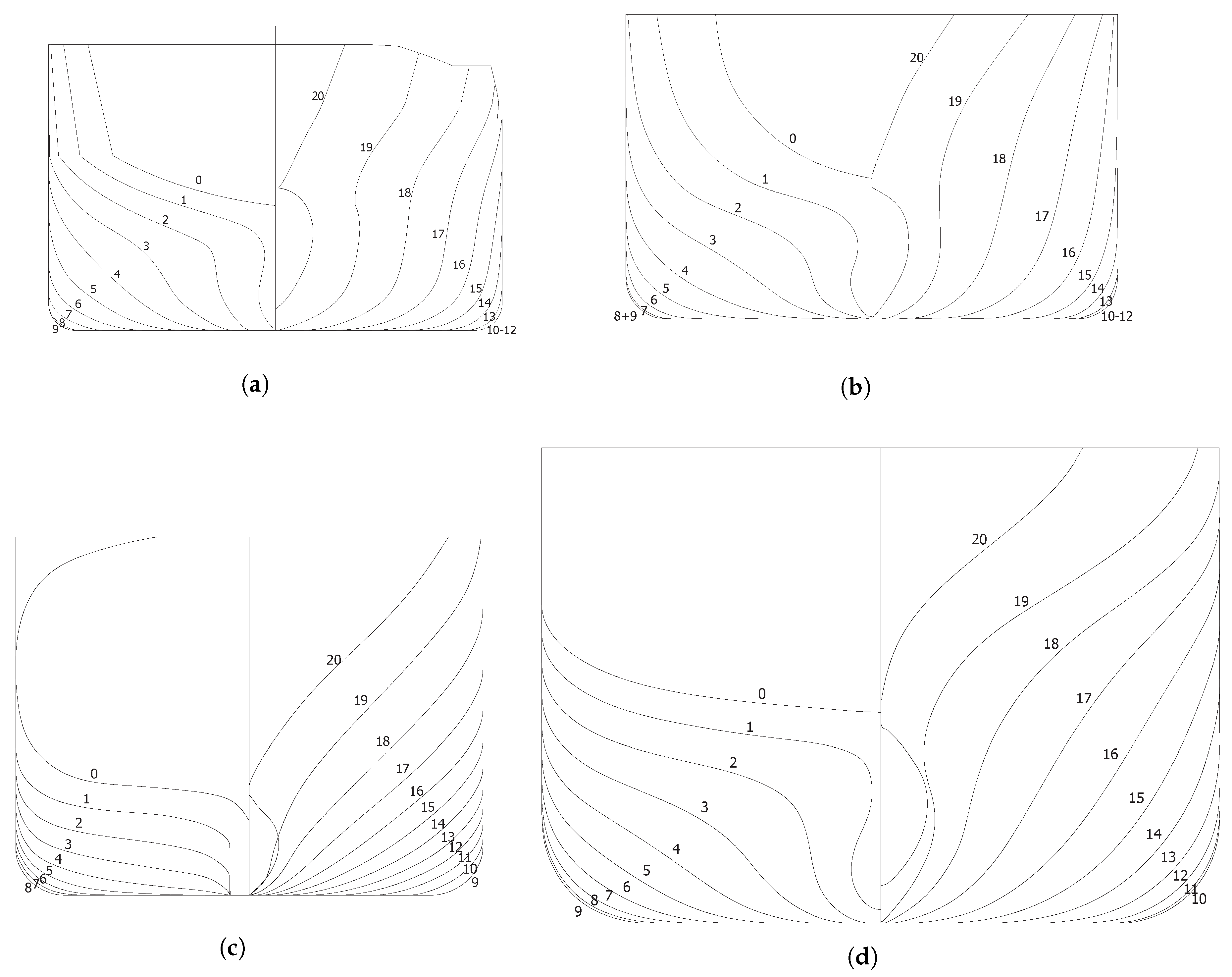
These four ships with their different bow and stern flares covered a broad range of hull forms. The ship lines for aft and forward sections are illustrated in Figure 1. Water depths of the model basins differed significantly. At CEHIPAR basin, water depth was 5.0 m; at TUB basin 1.0 m. Furthermore, models investigated at CEHIPAR were self-propelled; models tested at TUB were kept on position with soft springs.
4. Computational Setup
4.1. Strip Theory Method
Time-domain strip method computations were performed by IST for the cruise ship, the LNG carrier and the chemical tanker. Transverse strips distributed along the overall ship lengths idealized their hulls. Two-dimensional computed added mass and damping coefficients for each strip are integrated over the ship’s length to yield approximate three-dimensional added mass and damping coefficients for each ship hull. The hull of the cruise ship, for example, was represented by 38 strips, and each strip was approximated by 46 straight line boundary elements extending from keel to second deck. For these time-domain strip theory computations, a time step size of 0.1 s was selected to ensure convergence of ship responses in irregular seaways of three hours duration. Each seaway was composed of at least 1000 harmonic wave components. Regular waves and irregular sea states were computed for the comparative study. The simulated irregular sea states were reconstructions of the experimental sea state realizations. Heave, pitch and surge motions were computed for regular and irregular waves computations.
4.2. Rankine Source Boundary Element Method
Computations with the Rankine source boundary element method were performed by DNV GL for three ships, namely the cruise ship, the chemical tanker and LNG carrier. Structured surface meshes discretized the hulls and the free surface. The overall number of panels varied between 4000 and 6000. Panel sizes depended on wave lengths (regular waves) and significant wave lengths (irregular waves) tested. Typically, at least six panel lengths equaled the shortest expected wave length. This yielded a panel length near the hulls of about 2.4 m. Finite water depth, if needed, was accounted for by additional Rankine functions. The potential distribution on the boundaries was described by B-spline patches. The time step size applied varied between 0.01 and 0.10 s. Between 100 and 200 harmonic wave components were superposed to establish an irregular seaway. Heave, pitch and surge motions were computed for regular and irregular waves computations.
The simulations with irregular seas were conducted with random realizations and do not match the exact sea state realization applied in the model tests. As a consequence, time series of wave elevation and ship responses can not be compared.
4.3. Field Method
Field method computations were performed for all four ships. We used a Cartesian coordinate system S (x, y, z) fixed to the ship’s body. Its x-axis is directed forward, its y-axis to backboard, and its z-axis normal to the plane decks upward. Its origin is at the centre of gravity G.
A large number of numerical simulations under various wave conditions were carried out. Different significant wave heights and zero-uprossing periods necessitated different grids with adapted grid topologies. The influence of the spatial and temporal discretization on nonlinear wave propagation and on ship responses in regular and irregular waves was extensively studied, discussed and published by the authors in [14,15]. This discretization study was the basis for the selected temporal and spatial discretization in this paper. For this reason, we refrained from performing a similar study here. The papers address the free surface elevation and ship responses in regular waves as well as the relative energy loss for different sea states and discretization levels at different distances from the inlet boundary. While ship motions and loads in regular waves are less sensitive to discretization errors, the free surface elevation depend significantly on the order of approximation as well on the discretization. Further on, it was found that discretization errors increase the energy loss (down stream) of irregular waves with high steepness defined as
with gravitational acceleration g. The difficulty to distinguish between energy loss related to wave-breaking and numerical diffusions was discussed.
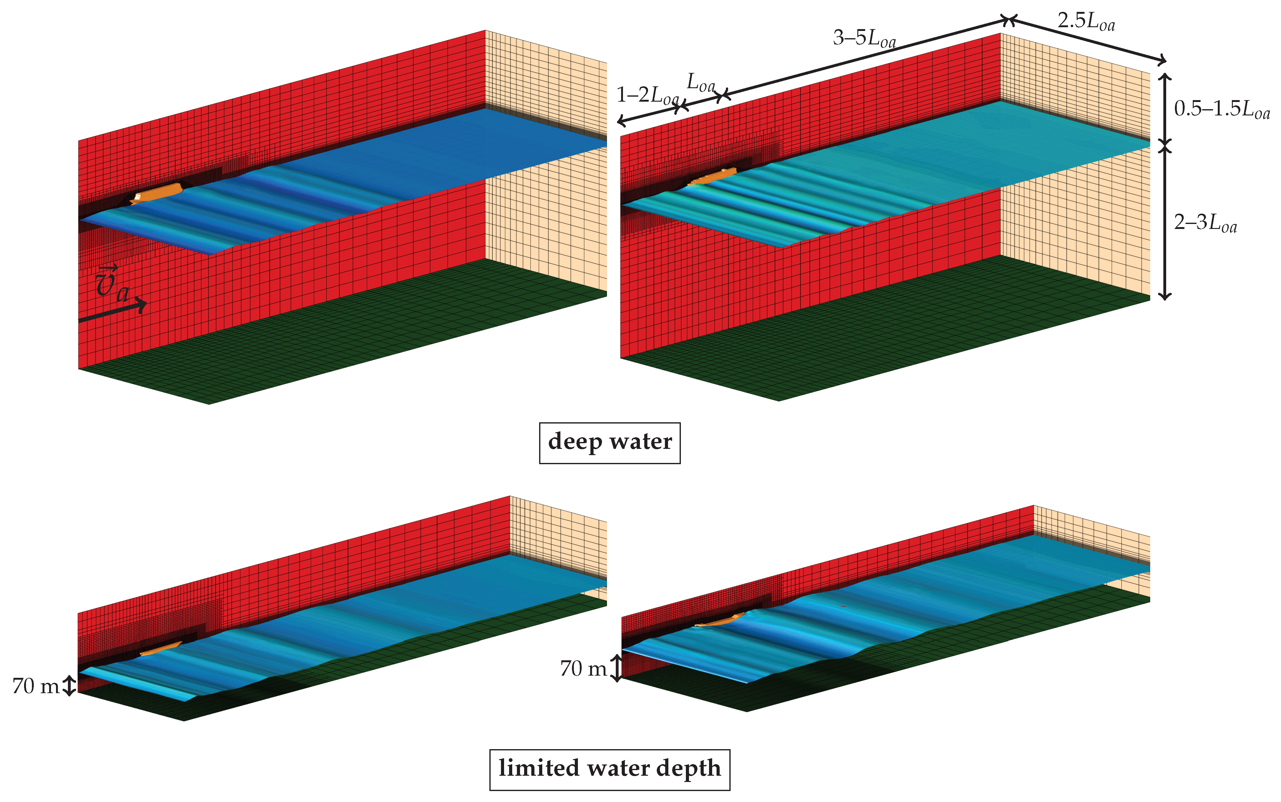
Common for all cases was the refinement area near the free surface ahead of the ships. A refinement box at and underneath the free surface resolved wave velocities, and pressure fields needed to be sufficiently fine to avoid loss of wave energy. The vertical extension of this refinement box depended on a sea state’s significant wave height and mean wave period. To capture the interaction between waves and hull, the refinement box around the hull had to be extended in the positive z-direction. The ships’ center plane defined a vertical symmetry boundary. Towards the far side of the domain (outlet), stretched cells and additional source terms dampened the waves. Figure 2 shows sample numerical grids for each ship, including simulated free surfaces for irregular long-crested waves and typical grid extensions as multiples of overall ship length, .
The effect of wave damping in vicinity to the outlet boundary is clearly visible. It starts about 1.5–2 times the ship length behind the model. Interfering effects of active wave damping on the simulation results can be ruled out. Model tests of the LNG carrier and the chemical tanker had to account for the limited water depth of the basin at TUB. Wave probes were mounted numerically to monitor the wave elevation at different locations.
Table 2 summarizes discretization parameters used for mesh generation. Cell lengths, , and cell heights, , indicate characteristic spatial resolutions and were related to the sea state parameters significant wave height (or regular wave height H), wave length , and peak period (or regular wave period T). Between 250 and 800 harmonic wave components were superposed to model an irregular seaway.
Surge motions were suppressed in regular wave simulations. For the cruise ship and containership sailing with forward speed in severe irregular seas, the surge motion was prescribed using the measured time signal of the physical self-propelled model1.
The simulations with irregular seas were conducted with equivalent sea state realizations as used in the model tests. Thus, time series and short-term statistics for wave elevation and ship motions can be compared with model test results, see Section 5.2.2 and Section 5.2.3.
4.4. Green Function Boundary Element Method
The Green function boundary element method was used to compute the RAOs for the four test case ships. We discretized the wetted hull surface using about 4500 surface panels and accounted for the limited water depth of the towing tank for the chemical tanker and LNG carrier. To investigate the water depth effects on ship responses, we performed additional computations under deep water conditions.
5. Results
The numerical methods were validated based on Froude-scaled model test results. The flow around ships in waves (and related vertical motions and loads) is pressure dominated. We can assume that viscous effects are negligible.
5.1. Regular Waves
For all four ships, systematic tests were conducted to obtain the ship response RAOs. As ship responses in regular waves with small and moderate heights were expected to be almost linear, deviations between numerical and experimental RAOs helped to quantify uncertainties in predictions of linear or weakly nonlinear responses before starting to address strongly nonlinear responses obtained in irregular seas. Not only biases and uncertainties that may have affected numerical predictions have to be taken into account, but also uncertainties in measurements and post processing of data.
Simulations and model tests were conducted in regular waves of constant steepness and varying wave period and in transient wave trains comprising harmonic wave components with amplitudes and frequencies in accordance with the spectral energy of a specified seaway. The latter approach significantly saves computational time; instead of simulating each wave period, only one simulation with a transient wave train is required.
Experiments and computations were obtained only in head waves () of varying frequencies, with the cruise ship and the containership advancing at a forward speed of 6.0 and 15.0 kn, respectively. The LNG carrier and the chemical tanker were investigated at zero forward speed. Evaluated responses comprised midships vertical bending moment, , pitch motion, , heave motion, and (partly) surge motion, , see Table 3.
5.1.1. Cruise Ship
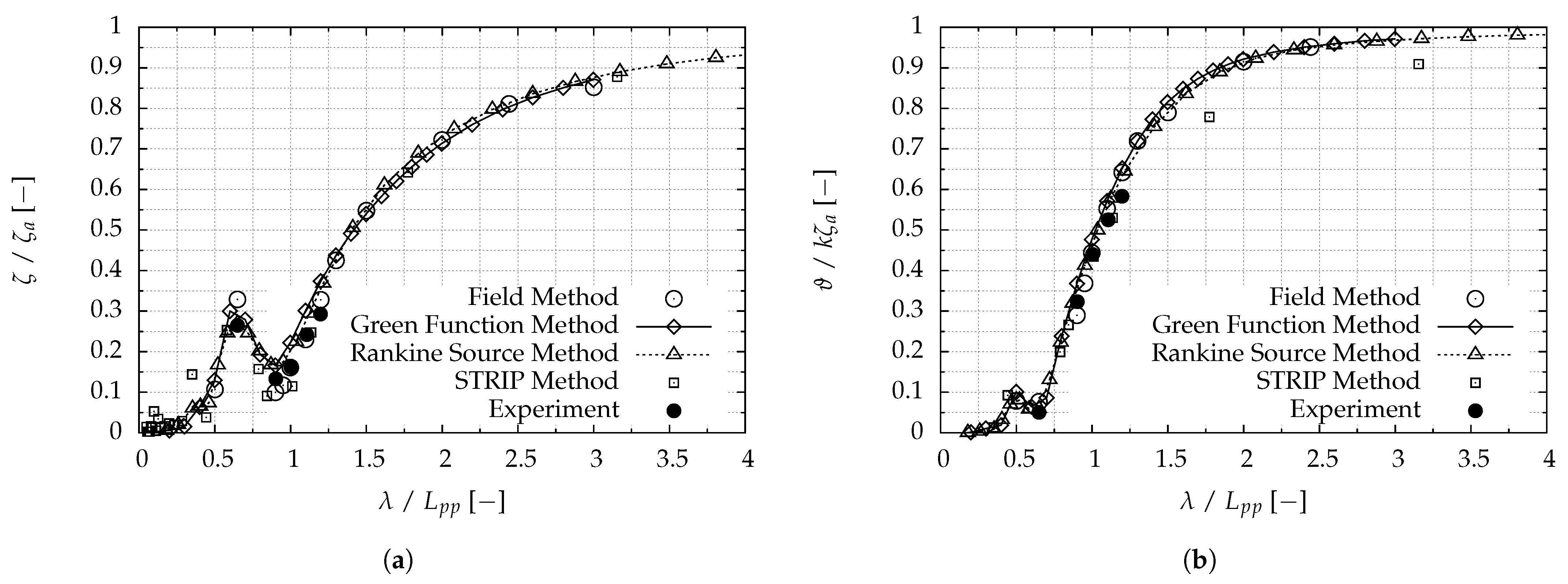
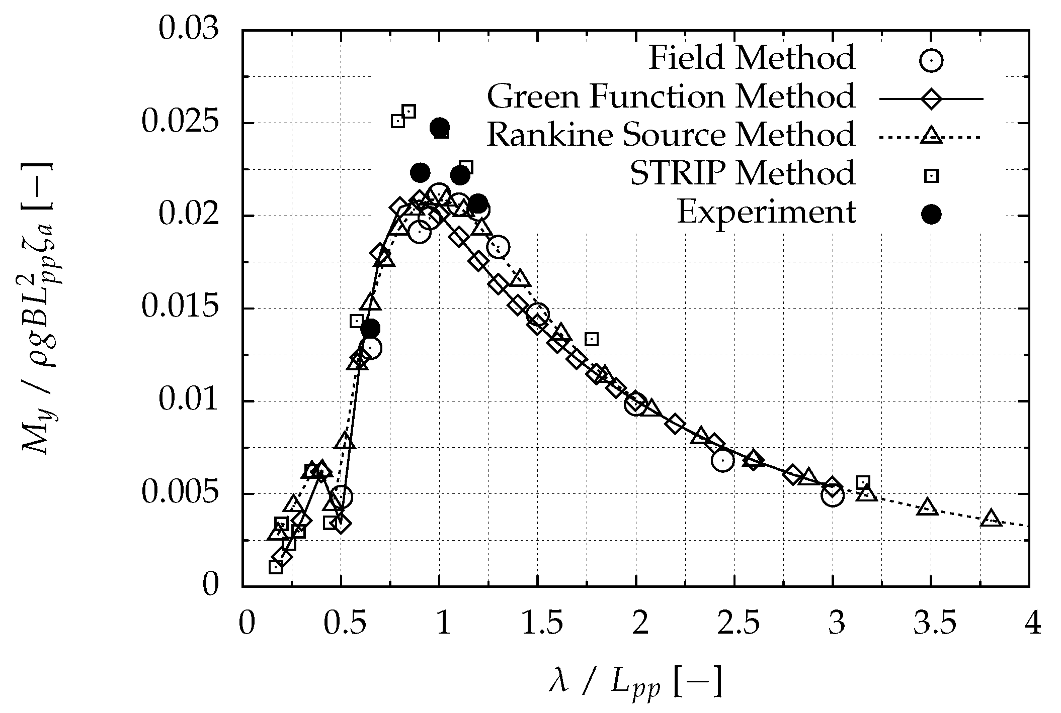
For the cruise ship, Figure 3 shows the resulting RAOs of heave and pitch motions; Figure 4 the resulting RAOs of midships vertical bending moment. Heave RAOs were normalized against wave amplitude, ; pitch RAOs against wave slope, ; vertical bending moment RAOs, against the product , where k is the wave number. The numerically predicted heave and pitch RAOs agree well with each other and with experiments. However, the strip method yields lower pitch motion amplitudes in longer waves. Comparative experimental data were unavailable for these wave lengths. The midship vertical bending moment RAOs were difficult to appraise. Although maximum values from field method, Rankine source and Green functions boundary element methods agree well, they are about 20% below measurements. Only results from strip method compare well to measured maximum bending moments. The measurements are characterized by a pronounced peak, whereas all numerical predictions (apart from strip method) have smoother slopes. Mismatches of ship model mass distributions might have caused the relatively large deviations of the maximum midship vertical bending moment RAOs. Since all heave and pitch motion RAOs generally compare favorably, poor performance of numerical methods was ruled out.
5.1.2. Containership
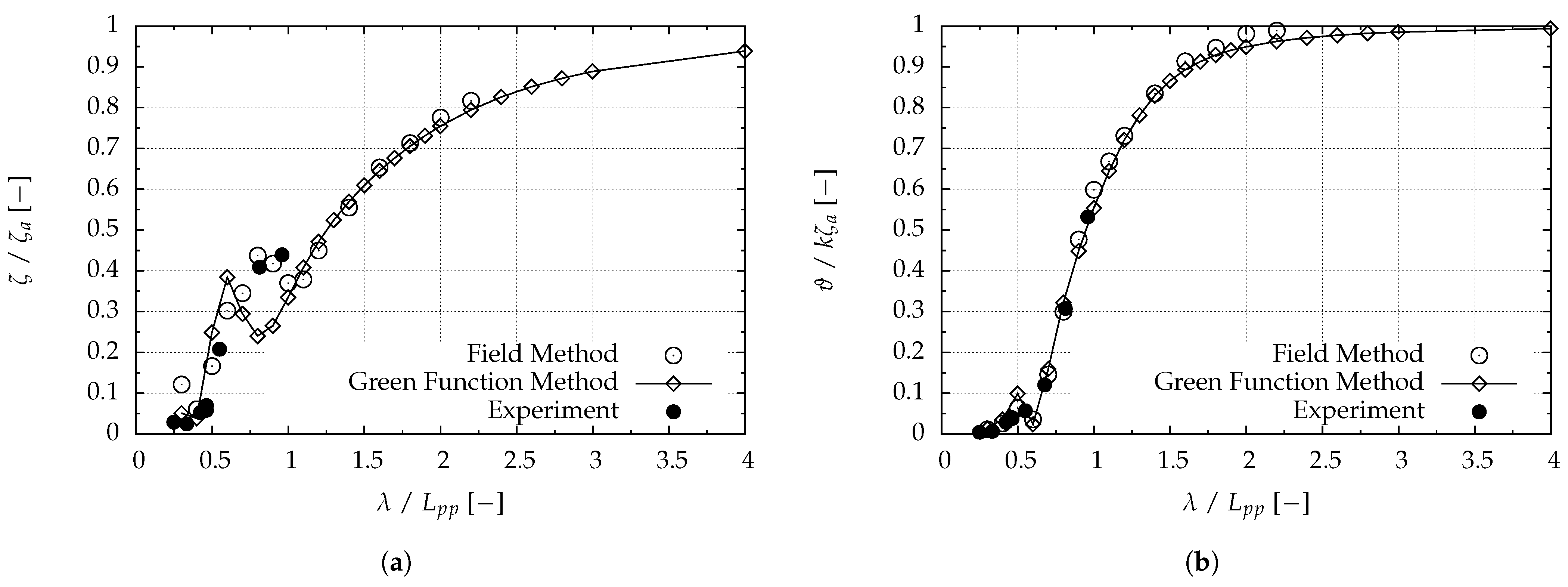
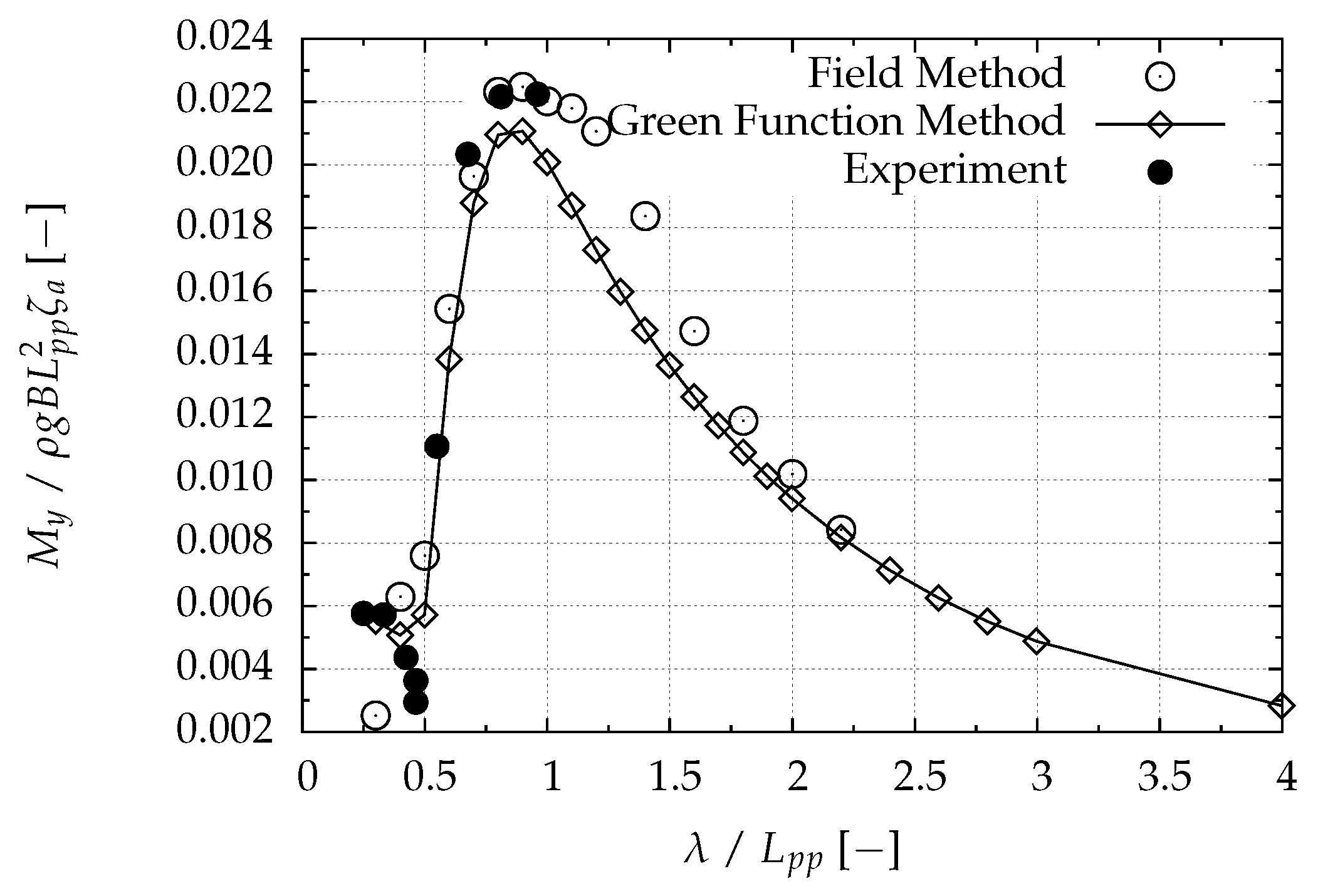
The containership model was equipped with a flexible backbone to measure the fundamental elastic behavior of the full-scale ship as described in Section 3. For the midship vertical bending moment, the low-frequency ship responses (without hydroelastic effects) were used for comparison of RAOs. Experimentally obtained time series of the ship advancing at a full-scale speed of 15.0 kn were analyzed. Comparative field method computations generally compare well to measurements, as seen by the heave and pitch motion RAOs shown in Figure 5 and the midship vertical bending moment RAOs shown in Figure 6. While the Green functions boundary element method computations predicted a local heave maximum at wave length to ship length ratio, , of 0.58, experimental and field method results indicate that this peak is shifted towards longer waves of close to unity. The discrepancy between the field method computed maximum RAO for the vertical bending moment and model test results was less than 2%, for the Green function method 7.5%.
5.1.3. LNG Carrier
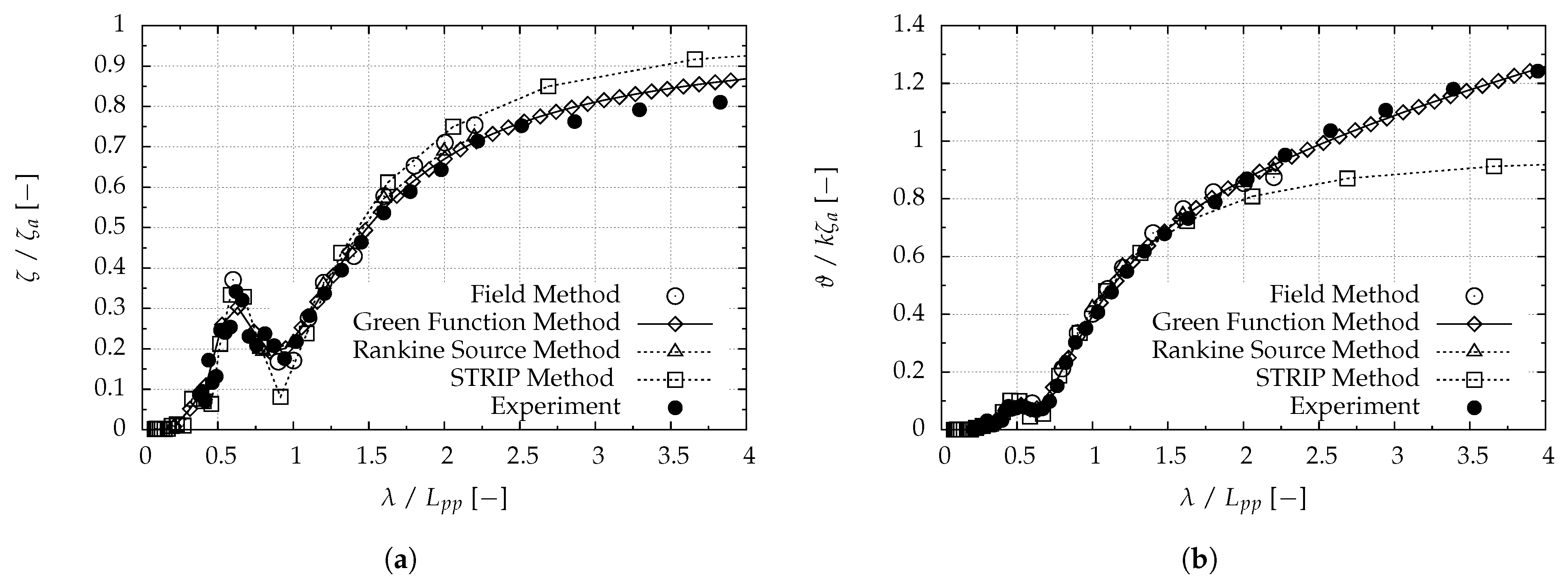
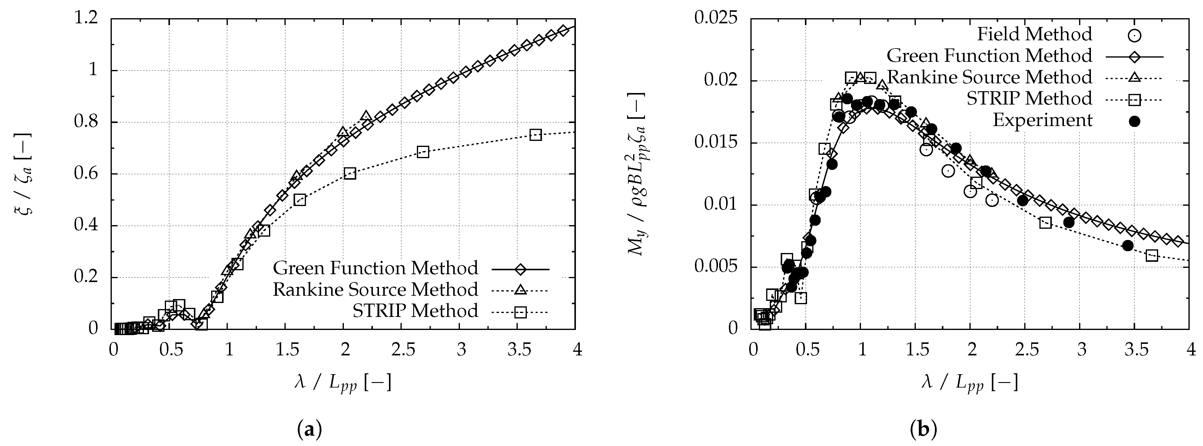
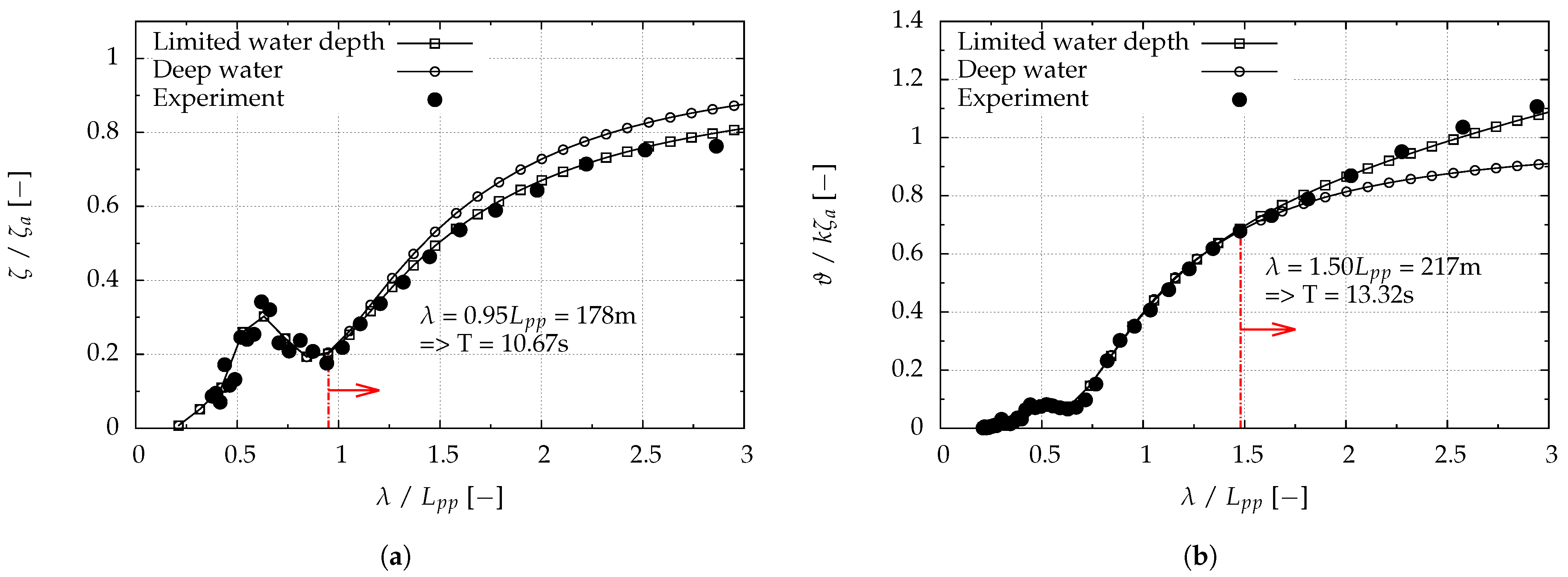
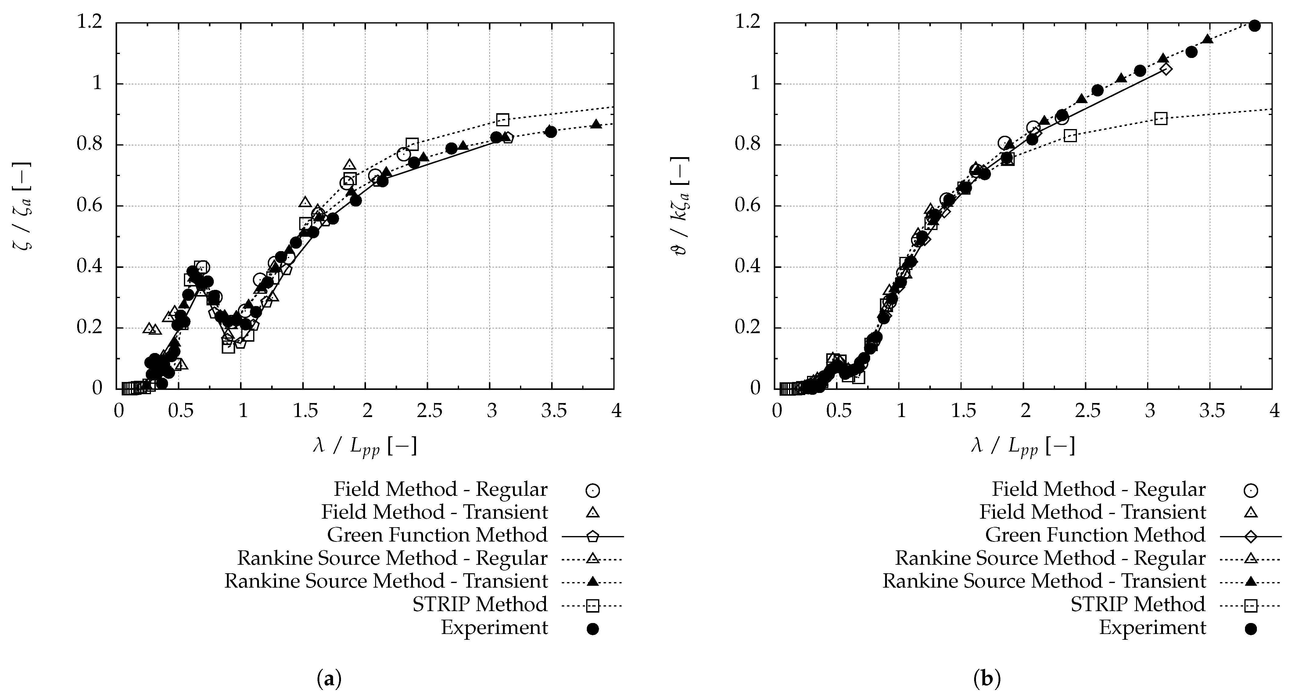
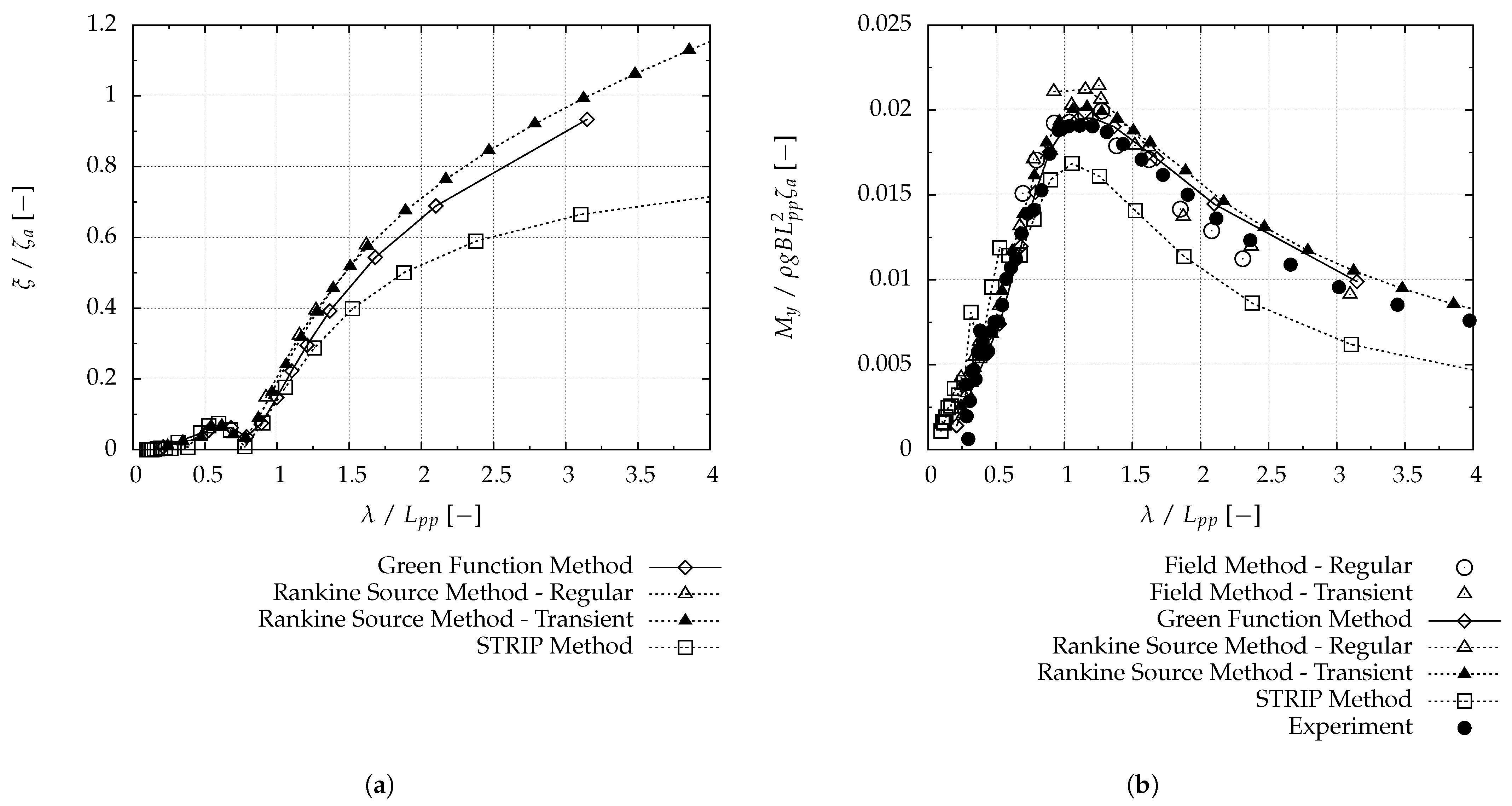
Figure 7 and Figure 8 show computed and measured RAOs of heave, pitch and surge motions as well as midship vertical bending moments. Numerically predicted maximum RAO values of heave, pitch and vertical bending moment from field method, from Green functions boundary element method and from Rankine source boundary element method agree fairly with experimental measurements. Comparable pitch and surge motions from strip method are underpredicted, while heave motions in long waves are overpredicted. This is caused by the neglection of shallow water effects. Computed maximum midship vertical bending moments using field and Green functions boundary element methods compare favorably with experimental data. The differences obtained are less than 3%. In shorter waves ( < 0.8), agreement between results obtained from all numerical methods is satisfactory, in longer waves the discrepancies increase. At a scale of 1:70, the model tests at TUB represent a water depth of about 70 m, which is less than 0.5 for the LNG carrier.
Additional comparative calculations for finite and infinite water depths were performed. Shallow water effects begin occurring at different wave lengths, depending on the ship response considered, see Figure 9 and Figure 10. Here, red lines mark the lower wave length limits where responses in finite water depth started to significantly deviate from responses in infinite water depth. While shallow water effects decreased the heave amplitudes in longer waves, pitch motions and midship vertical bending moment amplitudes increased. For wave lengths larger than , heave is already affected by the limited water depth, whereas pitch and surge start to visibly deviate from . When heave was influenced by shallow water, vertical bending moments are affected as well. This correlation appeared to be reasonable. Consistent with classical theory of gravity water waves and ship dynamics, water depth h starts to affect ship responses in waves for .
5.1.4. Chemical Tanker
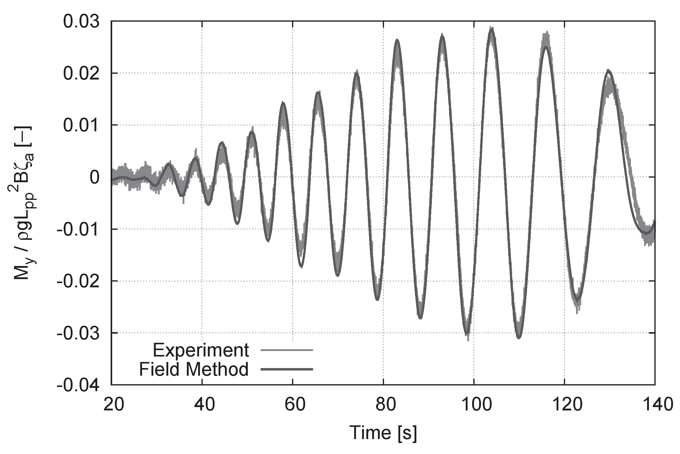
Figure 11 and Figure 12 show computed and measured RAOs of the chemical tanker responses. Except for strip method predictions of ship motions and midship vertical bending moment in long waves, numerical and experimental results agree well. This is valid for both concepts, single regular waves and transient wave trains. We carried out field method simulations for this ship in the same transient wave train as in the model tests performed at the TUB basin [54]. Figure 13 shows the measured and computed midship vertical bending moment. Agreement between computed and measured vertical bending moments is impressive, indicating that using a field method in wave trains to determine RAOs bears a great potential to reduce computation times because only one single run is required instead of a set of runs in regular waves. For ship responses dominated by restoring forces and small memory effects (such as heave, pitch and midship vertical bending moment), this example demonstrated the usefulness of this approach. Field method simulations of the chemical tanker accounted for shallow water effects.
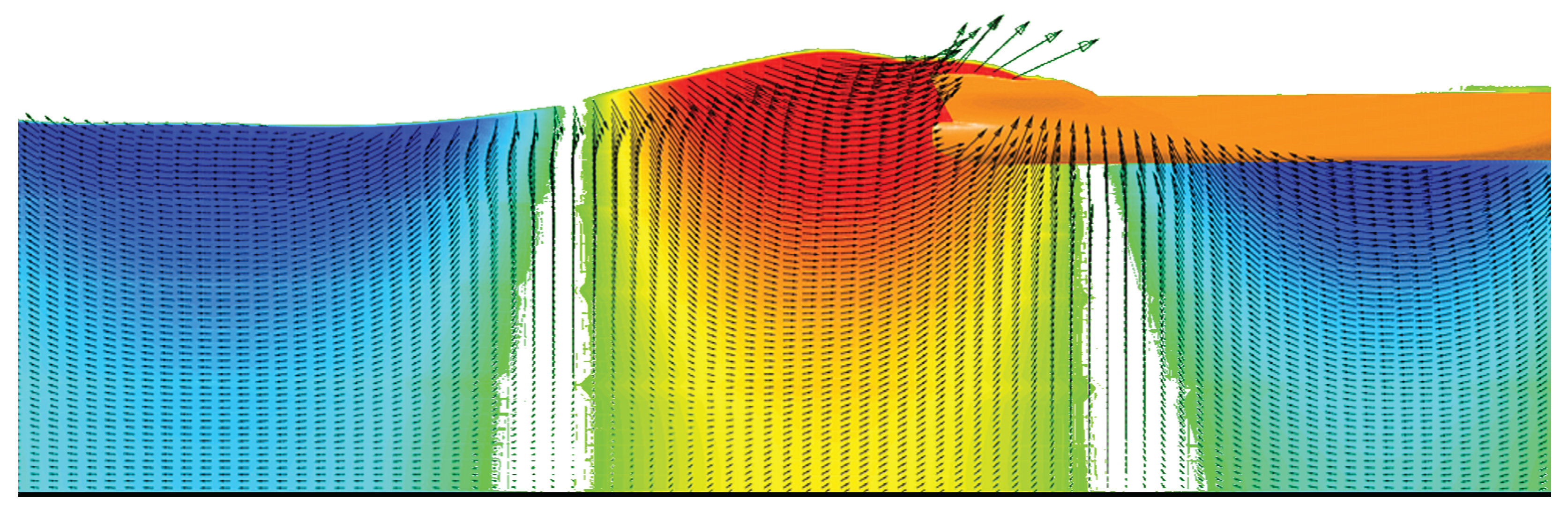
The exemplary vertical longitudinal cut through the fluid domain in Figure 14 shows pressure and velocity distributions while the ship encounters an extreme wave of about 15 m height and 200 m length. Pressure disturbances at the basin’s bottom caused by incident waves are visible, illustrating the influence of limited water depth on wave kinematics. The pressure field was obtained by subtracting hydrostatic (calm water conditions) pressures from total pressures. Red colored areas indicate positive pressures; blue colored areas, negative pressures. Black vectors represent velocity directions and magnitudes. Water depth corresponded to the basin depth of the experiments.
5.2. Irregular Extreme Waves
To assess the ability of the developed methods to predict ship responses in extreme seas, reliable predictions of short-term response statistics of the four investigated ships in irregular seaways were thought to be the best measure.
Usually statistical measures, such as the spectral energy density distribution, , describe an irregular sea state. Most common are the Pierson–Moskowitz spectrum [58] that only depends on wind speed, the modified Pierson–Moskowitz spectrum that depends on significant wave height and zero up-crossing wave frequency and the JONSWAP spectrum for limited fetch and wind duration [59]. The spectral energy density of the JONSWAP spectrum in is given as
with peak frequency , energy parameter , peak enhancement factor and shape factor . The parameter depends on the peak frequency :
For wave load predictions of ships, the International Association of Classification Societies (IACS) recommends the modified Pierson–Moskowitz spectrum, which corresponds to a JONSWAP spectrum with a peak enhancement factor of unity. By concentrating the wave energy in a smaller frequency band, an enhancement factor larger than 3.3 increases the modulation instability of sea states, promoting wave group formation with extraordinary high waves. When this frequency band coincides with frequencies relevant for ship responses, response amplitudes tend to be large compared with those in a sea state of the same energy but smaller enhancement factor.
Sea states are characterized by their peak period, , while their steepness is related to the zero-up-crossing period, , see Equation (1). The ratio of and depends on the peak enhancement factor and reads
Ocean waves are often not unidirectional; their energy is directionally spread about the principal wind direction. Although a cosine square distribution of wave energy over wave encounter angle is often assumed, the actual spreading strongly depends on wind conditions. Here, for the sake of simplicity, only head seas () were investigated. Based on the JONSWAP spectrum formulation, these random sea states were generated. The maximum peak enhancement factor used was 5.0.
5.2.1. Investigated Sea States
We used the Coefficient of Contribution method to identify each sea state’s relevance for long-term extremes of ship responses, thereby focusing the numerical and experimental investigations on sea states with large potential for extreme events. This screening relied on the linear three-dimensional Green functions boundary element method and wave statistics according to the IACS North Atlantic scatter diagram [60].
Table 4 lists the parameters identifying the irregular sea states investigated for comparative purposes. The run duration , i.e., the effective time the ship encounters the waves, is listed.
5.2.2. Time Histories
Time histories are the basis for statistical analyses. As described in Section 4, the strip method and the field method relied on reconstructions of experimental sea state realization. These reconstructions were based on wave probe measurements during the tests, safeguarding the best possible identity of wave processes in model tests and computations, eliminating uncertainties in numerical wave modeling and improving correlation of numerically and experimentally predicted ship response processes.
The boundary element method did not allow using replicas of the experimental wave processes. Instead, random sea state simulations based on the sea state parameters of the experiments had to be used. This made direct comparisons of time histories impossible.
In addition to ship responses, the incident wave elevation, , at the ships’ midship position was monitored to relate ship responses to the wave excitations and to assess the numerical wave models. This was of interest in sea conditions in which significant nonlinearities of the wave process were expected. Furthermore, surface elevation monitoring enabled assessing the numerical damping of waves likely to occur in field method simulations. This section shows exemplary results obtained for the cruise ship and the LNG carrier.
Cruise Ship
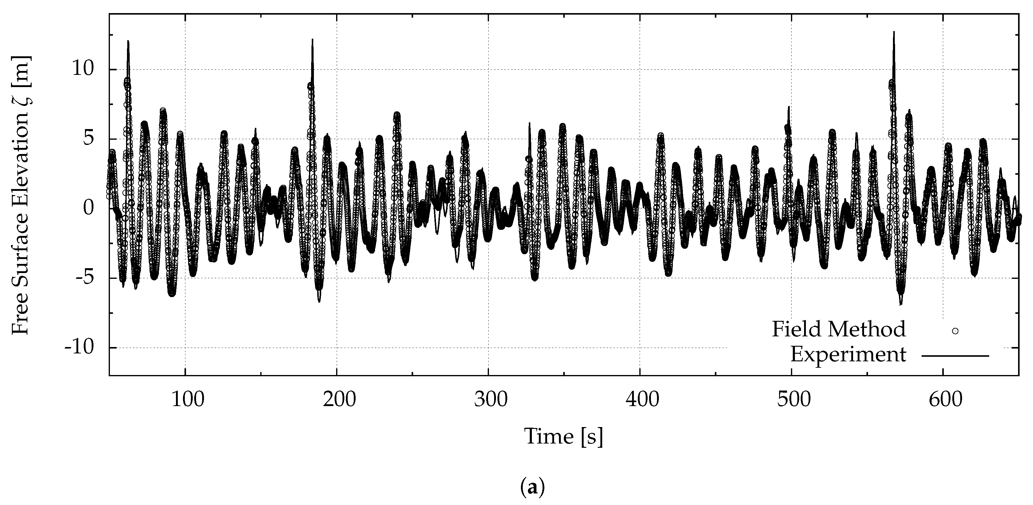
Figure 15 shows the computed and measured free surface elevation and the vertical bending moment amidships. As the free surface elevation obtained in the experiments is predefined in the STRIP method, the corresponding time history is not shown. The field method solves the nonlinear wave propagation inside the computational domain. Hence, the resulting wave field is of interest and compared with measurements.
Except for a few events, a satisfying agreement between measured and computed free surface elevation as well as the corresponding wave-induced motions and bending moment was obtained, see Figure 15 and Figure 16. There is a good agreement in terms of phasing and amplitudes between measurements and field method computed results.
The comparison between strip method results and model tests reveals a favorable agreement in phasing and small ship response amplitudes as well. For moderate and large ship motions and loads, the deviations increase. In principle, large motion and load amplitudes are overestimated. Sagging moments (positive values) agree better than hogging moments (negative values) with model test results.
LNG Carrier
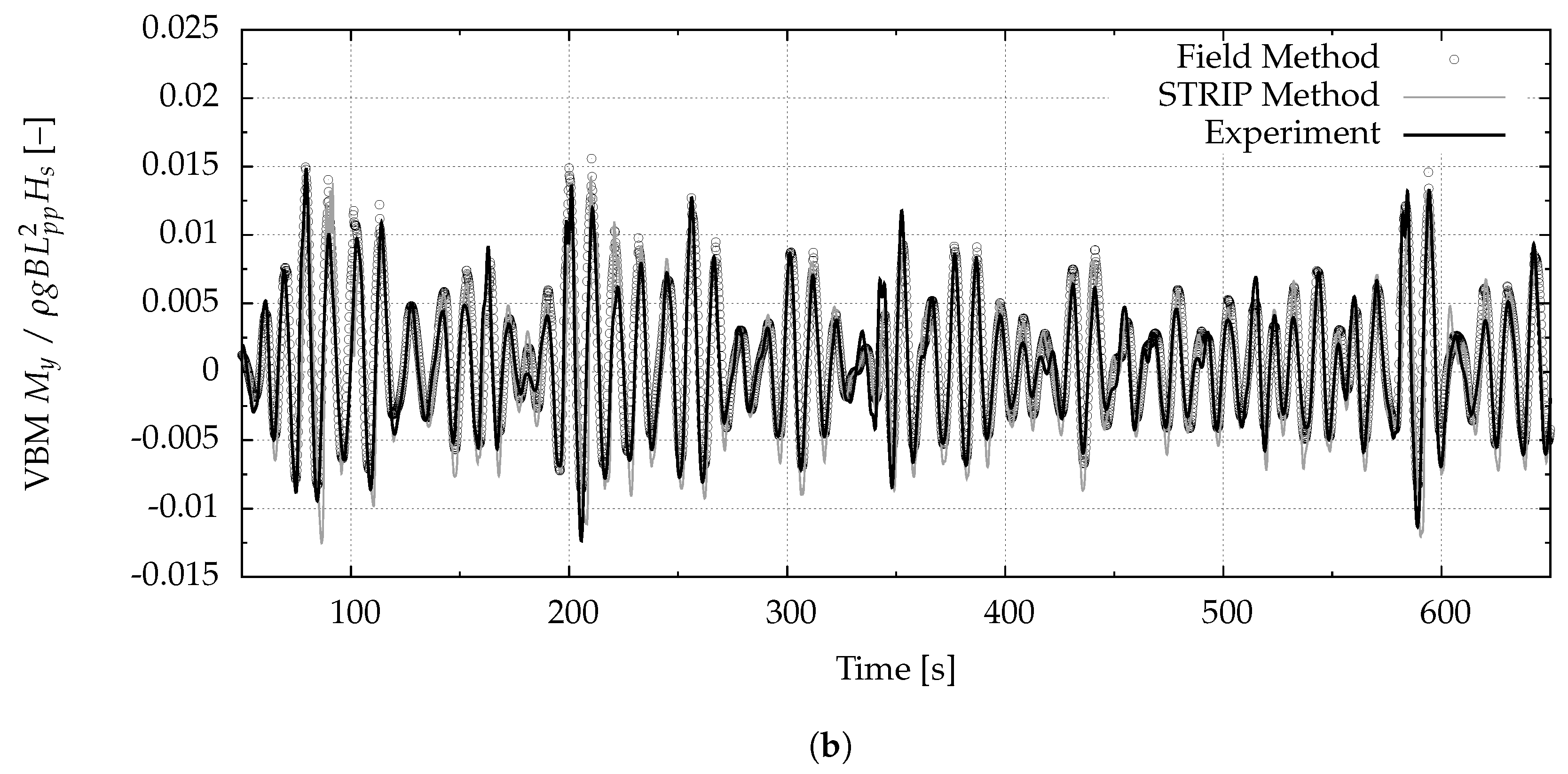
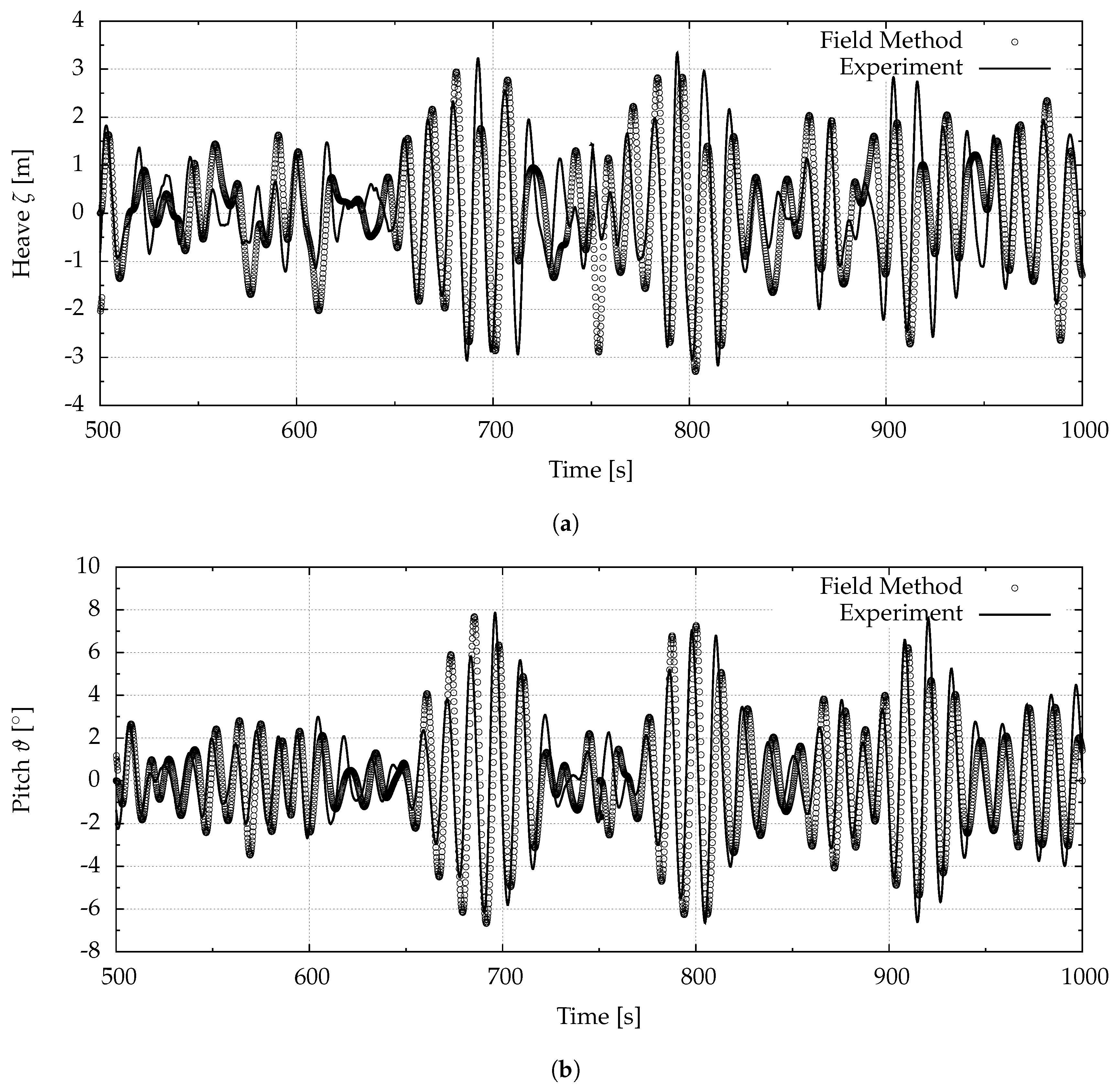
For the LNG carrier, the field and Rankine source method were employed to simulate ship responses. Solely the field method, however, reconstructed the equivalent model test sea state realizations. Figure 17 and Figure 18 show sample time histories of corresponding free surface elevations, ship motions and midship vertical bending moments in irregular waves. The selected time interval covered three severe wave groups. The field method captured the asymmetry between wave crests and troughs. Although differences of wave elevation and ship responses between model test and numerical results are most pronounced for heave, the overall agreement is satisfactory.
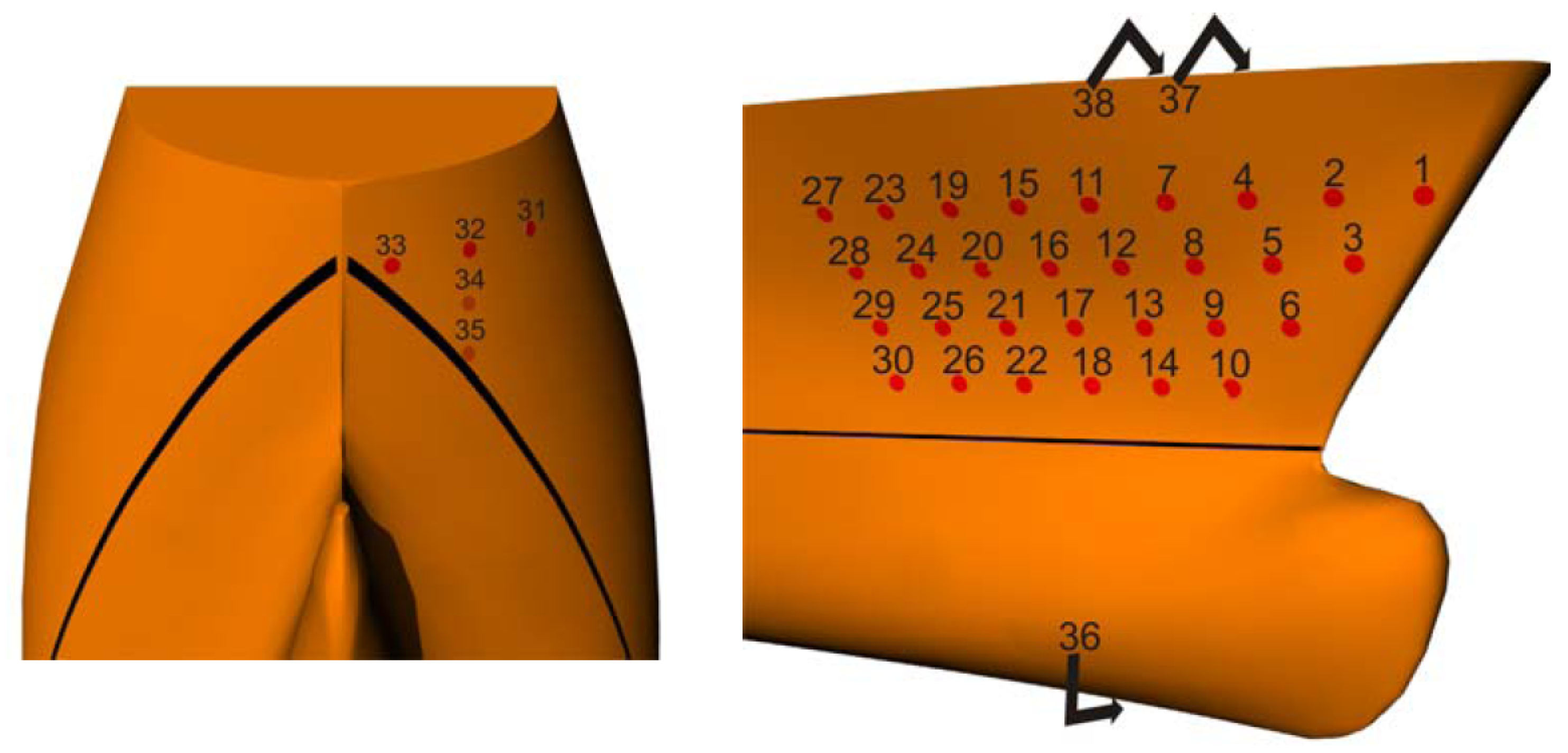
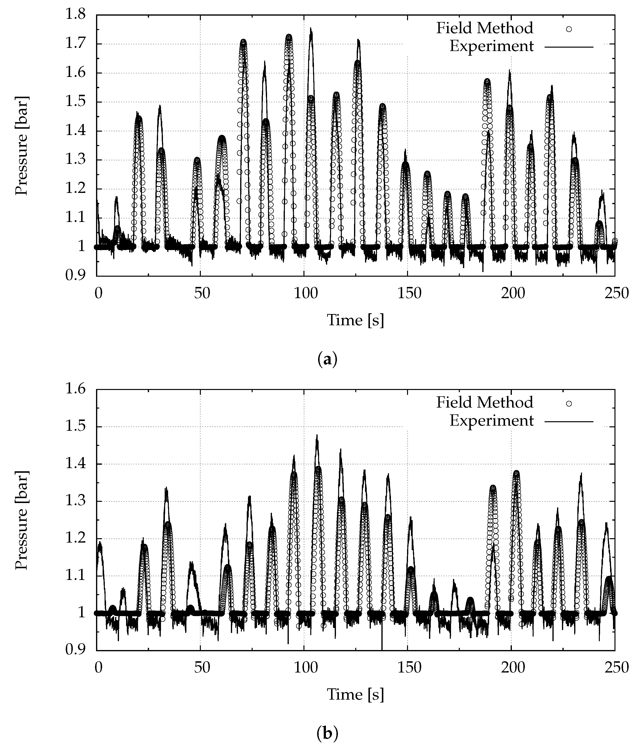
Pressures were measured using pressure sensors located at the ship’s stern and bow as shown in Figure 19. Figure 20 presents two exemplary time histories of pressures obtained from sensor 34 at the stern and senor 10 at the bow. Pressures included the atmospheric pressure of one bar. Due to zero forward speed and relatively small bow and stern flares, pressures were moderate, and no distinct slamming peaks occurred during the time interval considered.
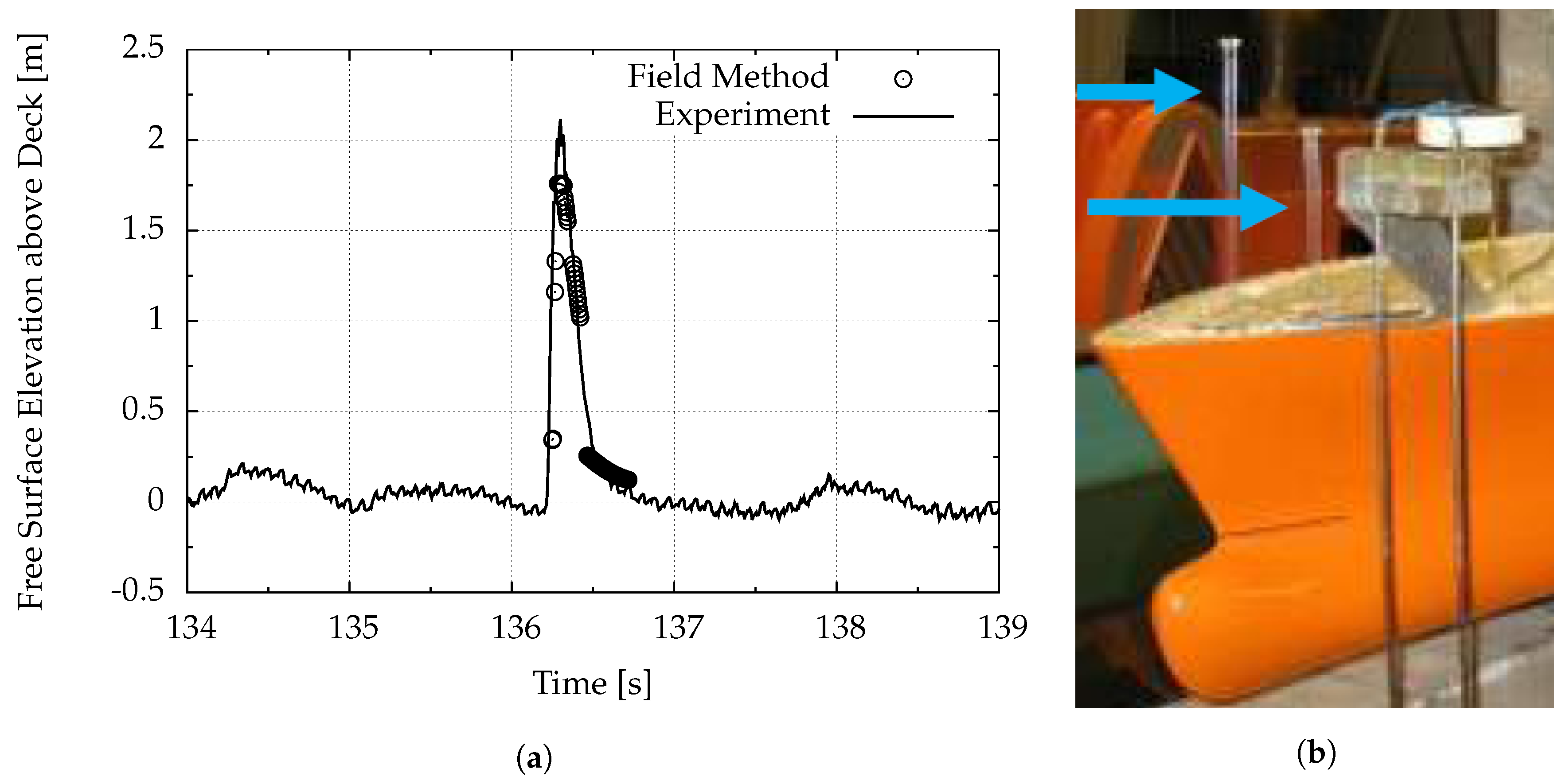
The green water column height above the weather deck was measured during experiments and monitored in numerical simulations. They agreed favorably over the time duration of such an event, as exemplarily shown in Figure 21. Here, the height of the computed water column is about 18% below the measured height. Considering the difficulties associated with determining the free surface elevation of a breaking wave and with a capacitance wave probe to accurately measure the water column height, the agreement was unexpectedly favorable.
5.2.3. Short-Term Statistics
Response peaks were identified from time histories as maxima and minima between consecutive zero up-crossings of a response process. Rainflow counting yielded exceedance rate distributions of response cycles (double amplitudes). The exceedance rate, , is the average frequency (unit [1/s]) of r being larger than . Evaluation was done for discrete response classes . Assuming that , the zero-upcrossing period of the process, is also the mean period of amplitudes due to the narrow-bandedness of the process, with probability P the rate of amplitudes outcrossing reads
Hence, gives the expected number of amplitudes larger than during a time interval .
Cruise Ship
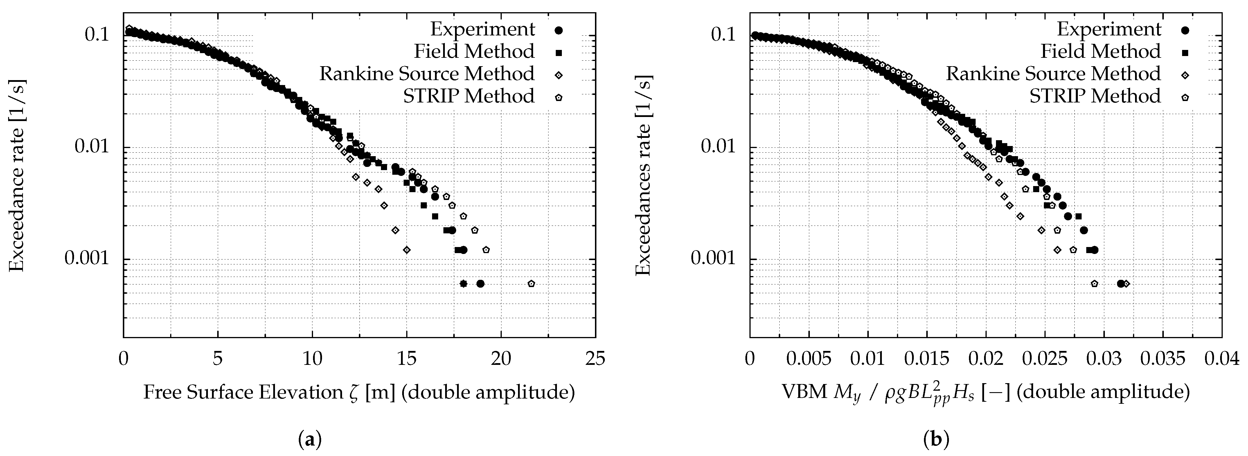
Short-term statistics were obtained for the cruise ship in irregular sea states with each numerical method. Figure 22a shows exceedance rates of incident wave elevation obtained by the range-pair counting approach, based on a sampling interval of about 27 min in irregular waves, see Table 4. Maximum wave heights reached up to twice the significant wave height. Wave elevation statistics based on strip theory were measured amidships; wave elevation statistics based on the Rankine source BEM and the field method, ahead of the ship. Except for tail distributions, range pair counted wave heights from all codes compare well with experiments although this method provided no information about mean values. Figure 22b shows exceedance rates of wave-induced vertical bending moments. The field method replicates the trend for low, moderate and large response levels. Good agreement was obtained with the BEM for low and moderate response levels. Deviations at the tail were probably caused by the sampling variability. Strip method predictions for small amplitudes agreed favorably with measurements; moderate and large bending moment amplitudes, however, deviated significantly.
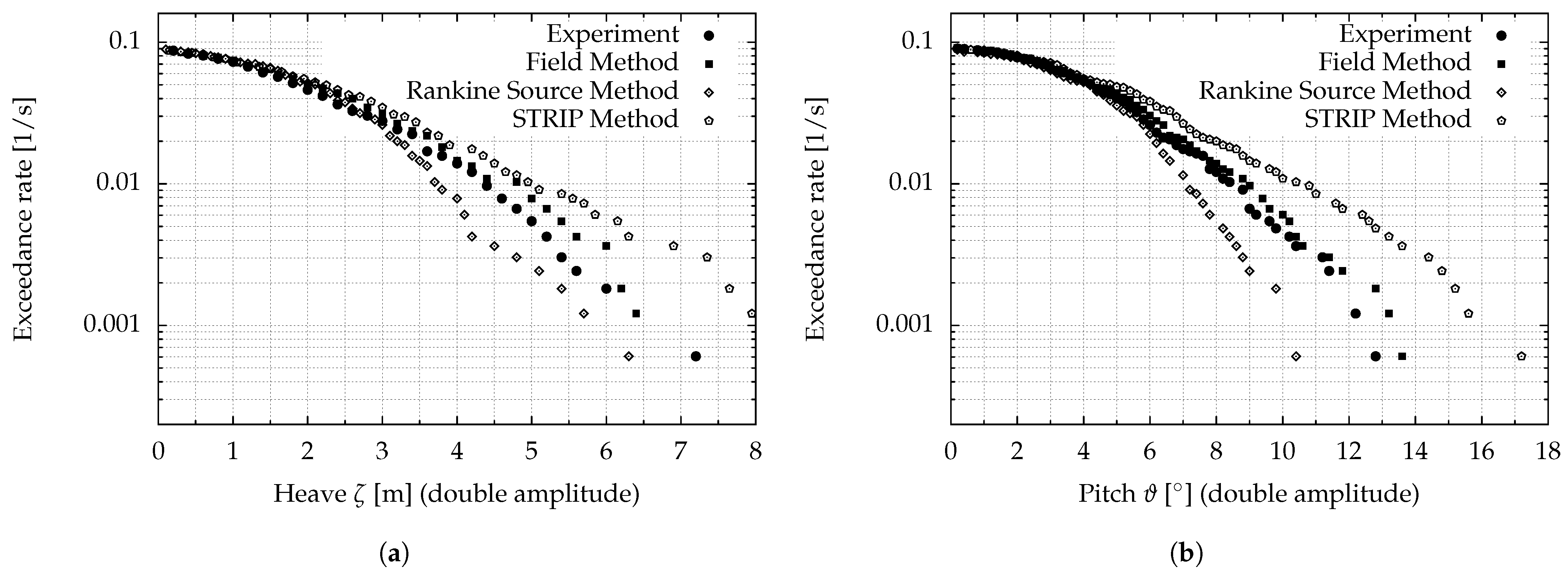
Figure 23 shows exceedance rates of heave and pitch, respectively. The field method obtains the best overall agreement with experiments, while the strip method overpredicts these motions already at moderate response levels although the midship vertical bending moment deviations are smaller. However, this is in agreement with previous comparisons. The BEM underpredicts these motions. Again, discrepancies are most significant in the tails of the distributions.
Chemical Tanker and LNG Carrier
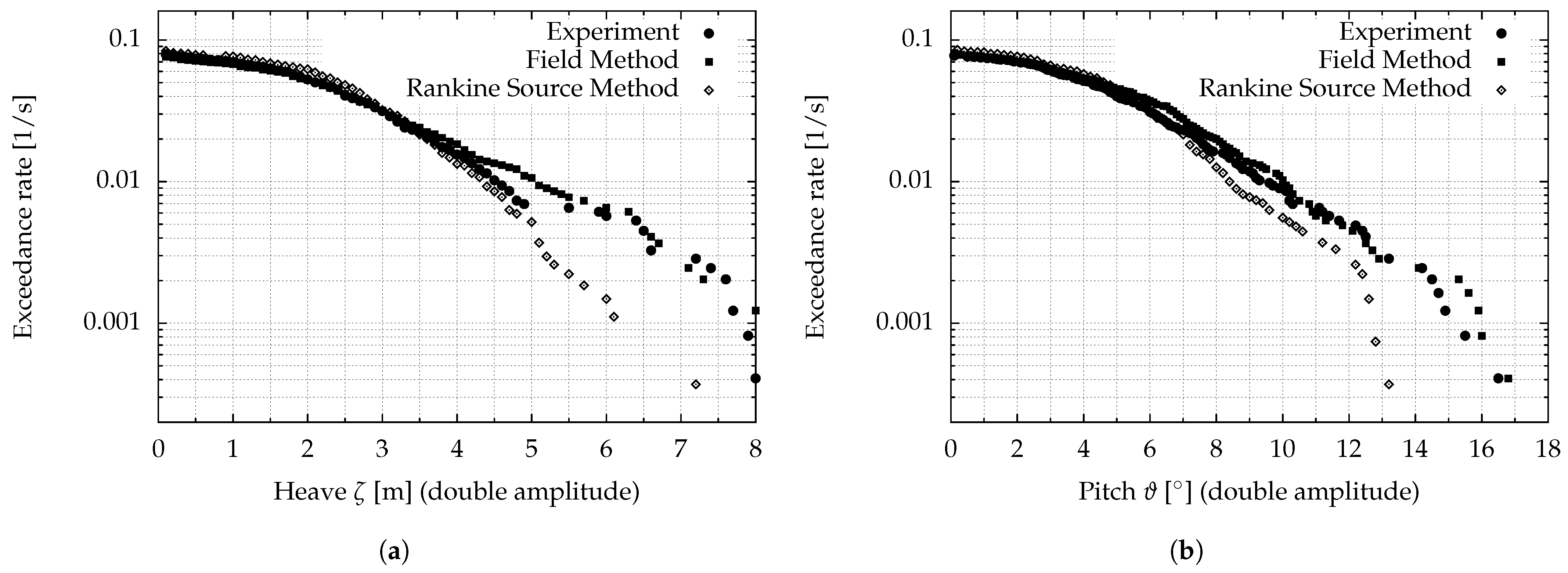
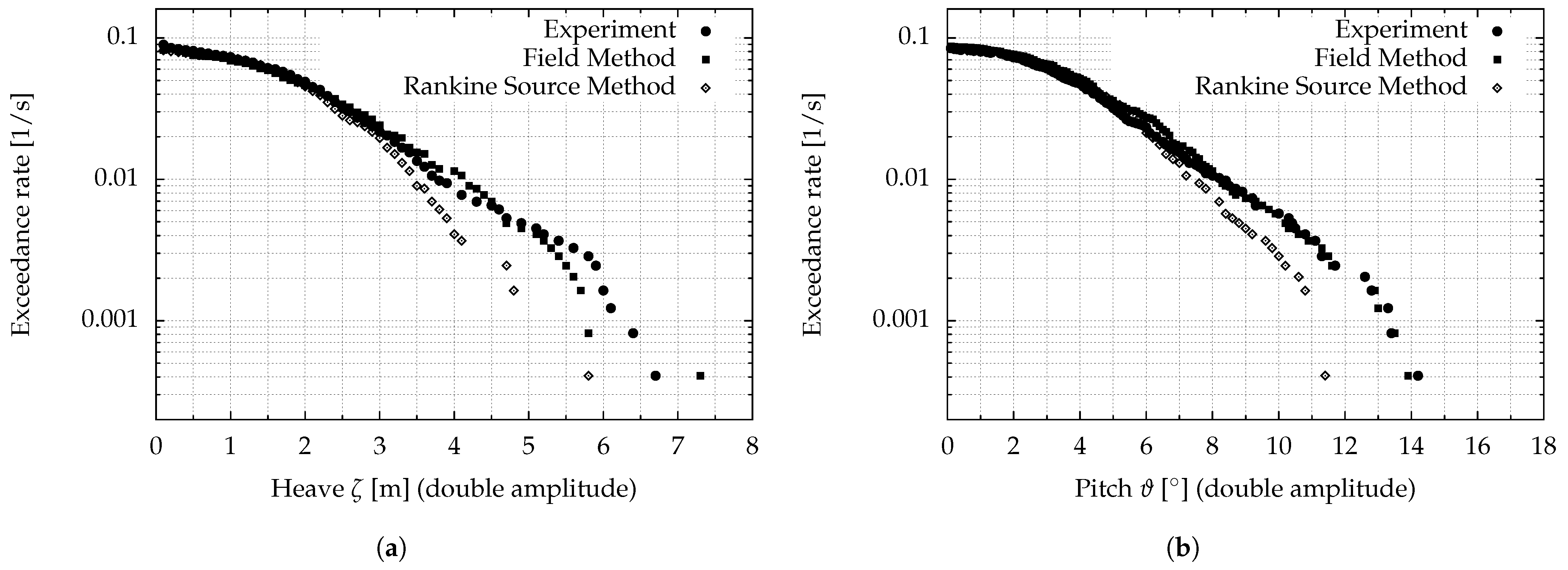
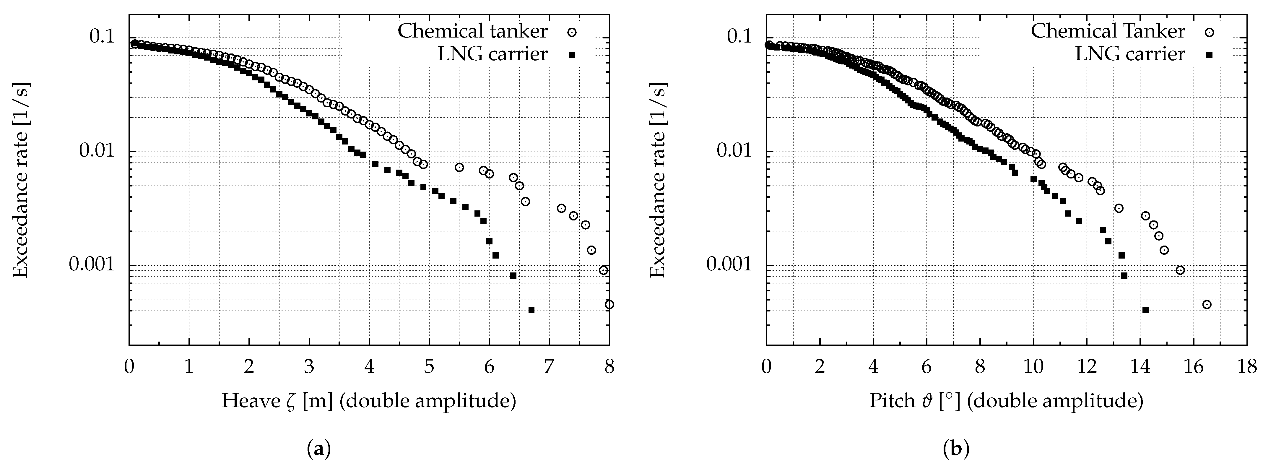
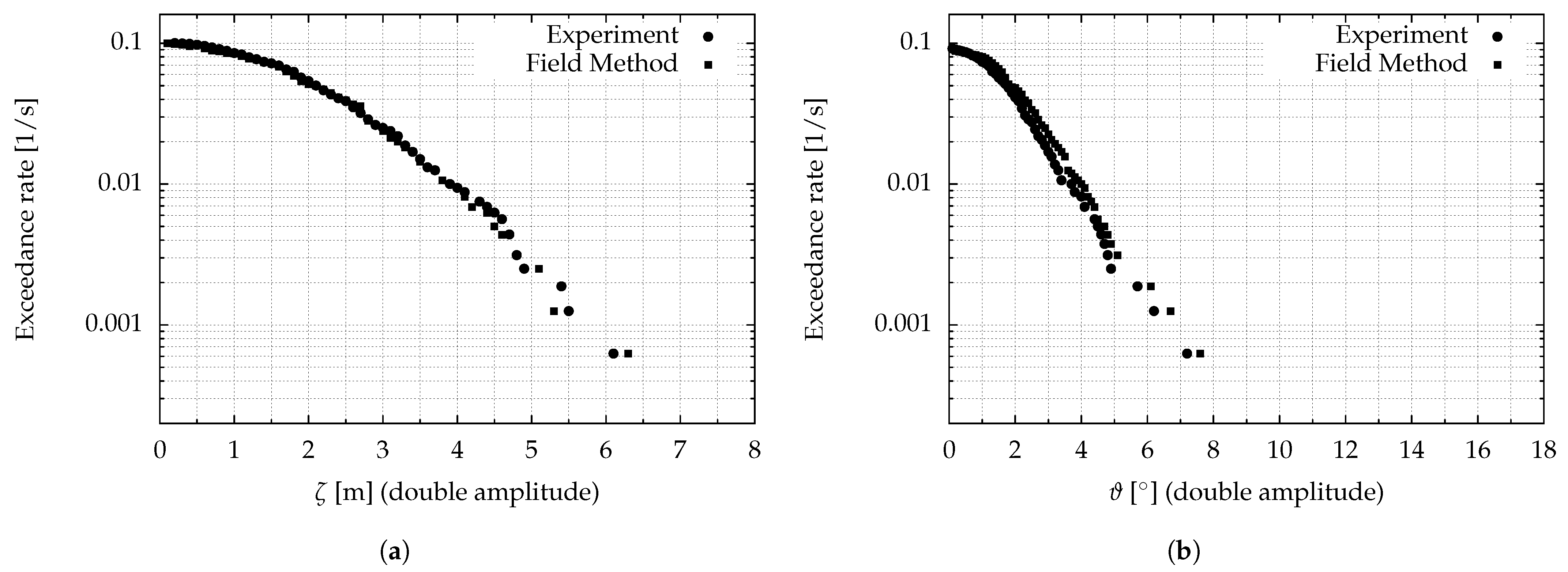
The chemical tanker and LNG carrier were analyzed using the field method and the Rankine source method, see Table 4. The corresponding model tests employed equivalent sea state realizations which allow for direct comparisons of ship responses. In accordance with Table 4, the time duration of the irregular sea was 45 min. Simulation results for heave and pitch motions are compared with model test results for both vessels and shown in Figure 24 and Figure 25. In both cases, field method computed heave and pitch motions fairly agree. Rankine source BEM computed and measured motions deviate notably.
Figure 26 shows a direct comparison of ship responses for the same sea states. Both ships were tested in different campaigns, but experienced the same waves (sea state realization). The pitch and heave motions are presented with absolute values. As expected maximum heave and pitch motions are remarkably stronger pronounced for the smaller chemical tanker and differ by about 19.4% and 17.1%, respectively. This trend is significant and starts at low response levels.
Containership
Short-term statistics were obtained for the containership in irregular sea states using field method and model tests. Range-pair counting yielded exceedance rates of ship responses both for the model tests and the field method numerical simulations. Computed and measured motions and the normalized vertical bending moments are compared.
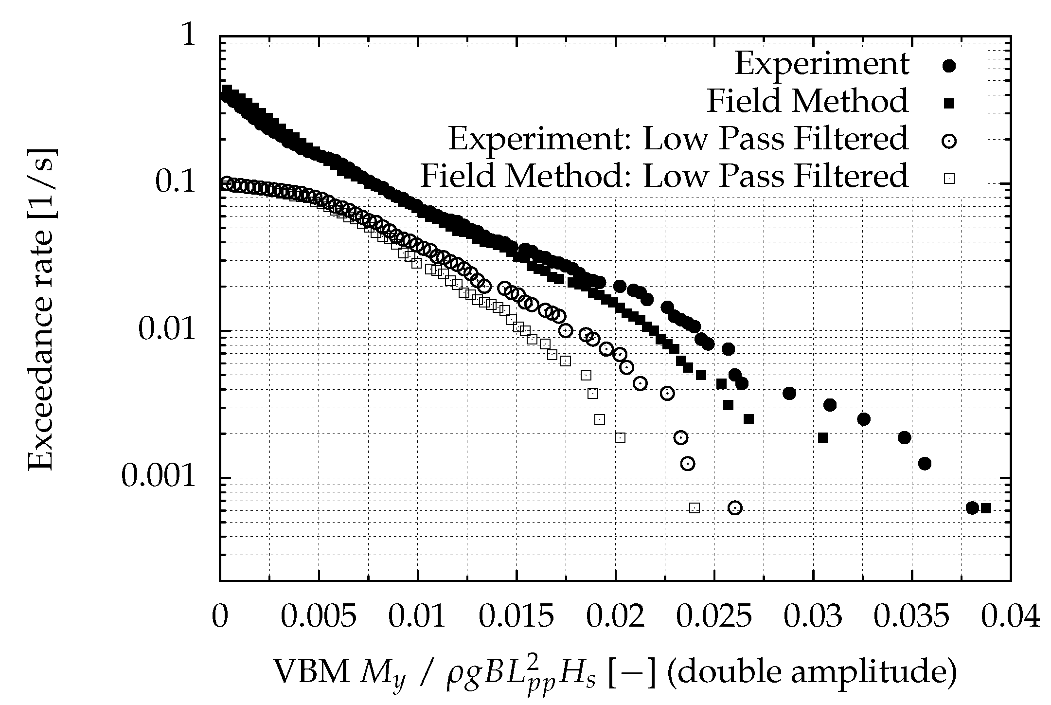
Heave and pitch motions agree satisfyingly, see Figure 27. The selected ranges for the horizontal axes equal those from the chemical tanker and the LNG carrier. Figure 28 plots the exceedance rates of midship vertical bending moment amplitudes. To eliminate the high-frequency vibratory part from the time histories, the response was low-pass filtered with a cut-off frequency of 0.25 Hz. The remainder was assumed to correspond to the rigid-body midship vertical bending moment.
There is a significant difference in the slopes of exceedance rates of both filtered and unfiltered signals. First, the number of response cycles increases dramatically due to hull girder vibrations. This is favorably replicated in numerical simulations. Second, the maximum response cycle obtained from the unfiltered signal is about 60% larger than the maximum response from the rigid hull signal. Numerically and experimentally determined exceedance rates basically show the same vibratory amplification; however, numerical results underpredict the responses at low exceedance rates. In general, numerical predictions of unfiltered data compare favorably with experimental measurements. Apart from the tail, the slope for low response levels is well reproduced.
6. Summary and Conclusions
We compared results obtained with enhanced seakeeping codes that were applied to numerically simulate ship response in regular and irregular severe seas. These codes were based on the strip theory method, the Green function method, the Rankine source boundary element method and a field method. Systematic comparisons of numerical results and model test data were carried out, focusing on response amplitude operators, time histories and short-term statistics. The resulting time histories and short-term statistics comprised responses in severe irregular sea states. Midship vertical bending moment, heave and pitch motions and free-surface elevations as well as pressure distributions and green water columns above deck were addressed.
The purpose was to assess the suitability of numerical methods to predict ship responses in regular waves and their short-term statistical measures under severe sea conditions and to provide benchmark data (free surface elevations, ship motions, loads, hydroelastic effects, pressures) for different ship types. Extreme sea conditions meant that nonlinear effects associated with wave propagation and wave-induced ship responses as well as the occurrence of wave grouping and wave modulation instability had to be considered. Furthermore, hull girder ship loads were affected by green water pressures and slamming impacts. For strip theory and boundary element methods, this application was challenging because of nonlinearities. Field methods are rarely used to compute short-term statistics of ship responses and hydroelastic effects in extreme irregular seas of long duration.
The four different ship types we investigated comprised three medium size ships (a cruise ship, an LNG carrier, a chemical tanker) and a large modern containership. In general, RAOs of ship responses (motions and loads) obtained from the numerical methods compared favorably to model test results. Viscous field methods were considered to be too time consuming and inefficient for the determination of RAOs. However, using wave trains (instead of single regular waves) increased the efficiency of field methods substantially.
The conformity of numerically and experimentally predicted time histories for the ships sailing in extreme waves demonstrated the principle suitability of the numerical methods applied here, namely, the strip theory method and the field method. Corresponding statistical distributions of free surface elevations, heave and pitch motions and vertical bending moments amidships were presented as double amplitudes. Significant wave heights varied between 10.5 and 12.5 m, which meant that maximum wave heights reached values of up to about twice the significant wave height. Each numerical method mentioned above was employed for the cruise ship. As expected, most promising results were obtained with field methods. However, the computational effort greatly exceeded that of potential theory based methods. An underestimation of extreme wave heights did not necessarily yield an underestimation of motions and vertical bending moment as predicted from the exemplarily presented time histories. In compliance with observations from RAOs and from time histories, short-term statistics revealed that motion (double) amplitudes were overestimated by the strip method in comparison with model test results. The vertical bending moment (double) amplitudes, however, agreed favorably. For the Rankine source boundary element method, large ship motion amplitudes, in contrast, were underestimated, whereas the vertical bending moment amidships also agreed favorably to model test results. A comparison of tail distributions, however, was inconclusive as these distributions were affected by the sampling variability of the random sea state realization. Trends described above applied to three ship types, namely, the cruise ship, the chemical tanker and the LNG carrier.
Finally, short-term statistics were presented for the containership. Not only the numerical field method, but also the experiments accounted for hull girder elasticity. Unfiltered and low-pass filtered signals were evaluated. As expected, the number of response cycles increased dramatically due to hull girder vibrations. The maximum response cycle obtained from the unfiltered signal was about 60% larger than the maximum response from the rigid hull signal. Numerically and experimentally determined exceedance rates basically showed the same vibratory amplification. Numerical predictions of unfiltered data compared favorably to experimental measurements. Apart from the tail, the slope for low response levels was well reproduced.
Based on the results presented above, we conclude that the Rankine source boundary element method as well as the nonlinear strip method are suitable to predict small and moderate ship responses. While the boundary element method underestimated extreme ship responses, the nonlinear strip method overestimated these extremes. Accounting for strong nonlinearities associated with impact-related slamming and green water loads in extreme waves required the use of a field method coupled with the nonlinear rigid body equations of motions and the linear equations of elastic body motions. The computational effort for this method was still high. However, it yielded the most promising ship responses over the entire range of wave conditions, extending from low amplitude regular waves to extremely large and steep irregular waves.
Author Contributions
Conceptualization, J.L. and O.e.M.; writing–original draft preparation, J.L. and O.e.M.; writing–review and editing, J.L. and O.e.M.; visualization, J.L. All authors have read and agreed to the published version of the manuscript.
Funding
The research leading to these results has received funding from European Union’s Seventh Framework Programme FP7-SST-2008-RTD-1 under grant agreement No. 234175.
Acknowledgments
Model tests presented in this paper were carried out at Canal de Experencias Hidrodinámicas Del Pardo (CEHIPAR), Madrid, and Technical University of Berlin (TUB), Berlin. The computations with the Rankine Source boundary element method have been carried out by DNV GL, Oslo, the strip theory method was applied at Instituto Superior Técnico (IST), Lisbon. The authors thank all contributors.
Conflicts of Interest
The authors declare no conflict of interest.
References
- International Union of Marine Insurance. 2016. Available online: http://www.iumi.com/ (accessed on 25 July 2020).
- Bishop, R.E.D.; Price, W.G. Hydroelasticity of Ships; Cambridge University Press: Cambridge, UK, 1979; ISBN 780521017800. [Google Scholar]
- Kahl, A.; Menzel, W. Full-Scale Measurements on a PanMax Containership. In Proceedings of the Ship Repair Technology Symposium Proc., Newcastle upon Tyne, UK, 1–2 September 2008; pp. 59–66. [Google Scholar]
- Storhaug, G.; Vidic-Perunovic, J.; Rüdinger, F.; Holtsmark, G.; Helmers, J.B.; Gu, X. Springing/Whipping Response of a Large Ocean Going Vessel—A Comparison between Numerical Simulations an Full-Scale Measurements. In Proceedings of the 3rd International Conference on Hydroelasticity in Marine Technology, Oxford, UK, 15–17 September 2003; pp. 117–131. [Google Scholar]
- Storhaug, G. Experimental Investigation of Wave Induced Vibrations and Their Effect on the Fatigue Loading of Ships. Ph.D. Thesis, Norwegian University of Science and Technology, Oslo, Norway, 2007. [Google Scholar]
- Vidic-Perunovic, J.; Jensen, J.J. Non-Linear Springing Excitation due to a Bidirectional Wave Field. Mar. Struct. 2005, 18, 332–358. [Google Scholar] [CrossRef]
- Hong, S.Y. Wave Induced Loads on Ships Joint Industry Project—II. In First Year Model Test Report; Technical Report No. BSPIS503 A-2112-2 (Confidential); MOERI: Daejeon, Korea, 2009. [Google Scholar]
- Hong, S.Y. Wave Induced Loads on Ships Joint Industry Project—II. In Technical Report No. BSPIS503 A-2207-2; MOERI: Daejeon, Korea, 2010. [Google Scholar]
- Hong, S.Y. Wave Induced Loads on Ships Joint Industry Project—III. In Technical Report No. BSPIS7230-10306-6; MOERI: Daejeon, Korea, 2013. [Google Scholar]
- Hirdaris, S.E.; Miao, S.H.; Price, W.G.; Temarel, P. The Influence of Structural Modelling on the Dynamic Behaviour of a Bulker in Waves. In Proceedings of the 4th International Conference on Hydroelasticity in Marine Technology, Wuxi, China, 9–13 September 2006; Volume 1, pp. 25–33, ISBN 7-118-04728-7. [Google Scholar]
- Hirdaris, S.E.; Temarel, P. Hydroelasticity of Ships—Recent Advances and Future Trends. Proc. IMechE Part M J. Eng. Marit. Environ. 2009, 223, 305–330. [Google Scholar] [CrossRef]
- Hirdaris, S.E.; Lee, Y.; Mortola, G.; Incecik, A.; Turan, O.; Hong, S.Y.; Kim, B.W.; Kim, K.H.; Bennett, S.; Miao, S.H.; et al. The Influence of Nonlinearities on the Symmetric Hydrodynamic Response of a 10,000 TEU Container Ship. Ocean. Eng. 2016, 111, 166–178. [Google Scholar] [CrossRef] [Green Version]
- El Moctar, O.; Oberhagemann, J.; Schellin, T.E. Free Surface RANS Method for Hull Girder Springing and Whipping. SNAME Trans. 2011, 119, 48–66. [Google Scholar]
- Oberhagemann, J.; Ley, J.; el Moctar, O. Prediction of Ship Response Statistics in Severe Sea Conditions using RANSE. In Proceedings of the ASME 31th International Conf. on Ocean, Offshore and Arctic Engineering, Rio de Janeiro, Brazil, 1–6 July 2012; pp. 461–468. [Google Scholar]
- El Moctar, O.; Ley, J.; Oberhagemann, J.; Schellin, T.E. Nonlinear Computational Methods for Hydroelastic Effects of Ships in Extreme Seas. Ocean Eng. 2017, 130, 659–673. [Google Scholar] [CrossRef]
- Hirdaris, S.E.; Miao, S.H.; Temarel, P. The Effect of Structural Discontinuity on Antisymmetric Response of a Container Ship. In Proceedings of the 5th International Conference on Hydroelasticity in Marine Technology, Southampton, UK, 7–9 September 2009; Volume 1, pp. 57–68, ISBN 9780854329045. [Google Scholar]
- International Ship and Offshore Structures Congress. In Proceedings of the 20th International Ship and Offshore Structures Congress, Amsterdam, The Netherlands, 9–14 September 2018; Volume 1.
- Hirdaris, S.E.; Bai, W.; Dessi, D.; Ergin, A.; Gu, X.; Hermundstad, O.A.; Huijsmans, R.; Iijima, K.; Nielsen, U.D.; Parunov, J.; et al. Loads for Use in the Design of Ships and Offshore Structures. Ocean Eng. 2014, 78, 131–174. [Google Scholar] [CrossRef]
- Newman, J.N. The Theory of Ship Motions. Adv. Appl. Mech. 1978, 18, 222–283. [Google Scholar]
- Faltinsen, O. Sea Loads on Ships and Offshore Structures; Cambridge University Press: Cambridge, UK, 1990. [Google Scholar]
- Söding, H. Ermittlung der Kentergefahr aus Bewegungssimulationen. Ship Technol. Res.-Schiffstechnik 1987, 34, 28–39. [Google Scholar]
- Jensen, J.J. Load and Global Response of Ships; Elsevier Ocean Engineering Book Series; Elsevier: Amsterdam, The Netherlands, 2001; Volume 4. [Google Scholar]
- Fonseca, N.; Guedes Soares, C. Time-Domain Analysis of Large-Amplitude Vertical Ship Motions and Wave Loads. J. Ship Res. 1998, 42, 139–153. [Google Scholar]
- Söding, H.; Shigunov, V.; Schellin, T.E.; el Moctar, O. A Rankine Panel Method for Added Resistance of Ships in Waves. J. Offshore Mech. Arct. Eng. 2014, 136, 031601. [Google Scholar] [CrossRef]
- Kim, Y.; Kim, K.-H.; Kim, Y. Springing Analysis of a Seagoing Vessel Using Fully Coupled BEM-FEM in the Time Domain. Ocean Eng. 2009, 785–796. [Google Scholar] [CrossRef]
- Sclavounos, P.D. Nonlinear Impulse of Ocean Waves on Floating Bodies. J. Fluid Mech. 2012, 697, 316–335. [Google Scholar] [CrossRef] [Green Version]
- Riesner, M.; Chillcce, G.; el Moctar, O.; Schellin, T.E. Rankine Source Time Domain Method for Nonlinear Ship Motions in Steep Oblique Waves. Ship Offshore Struct. 2018, 14, 295–308. [Google Scholar] [CrossRef]
- Riesner, M.; el Moctar, O. A Time Domain Boundary Element Method for Wave Added Resistance of Ships Taking into Account Viscous Effects. Ocean Eng. 2018, 162, 290–303. [Google Scholar] [CrossRef]
- Shao, Y.L.; Faltinsen, O.M. Numerical Study of the Second-order Wave Loads on a Ship with Forward Speed. In Proceedings of the 26th International Workshop on Water Waves and Floating Bodies, Athens, Greece, 17–20 April 2011. [Google Scholar]
- Papanikolaou, A.; Schellin, T.E. A Three-Dimensional Panel Method for Motions and Loads of Ships with Forward Speed. J. Ship Technol. Res. 1991, 39, 147–156. [Google Scholar]
- El Moctar, O.; Brehm, A.; Schellin, T.E. Prediction of Slamming Loads for Ship Structural Design using Potential Flow and RANSE Codes. In Proceedings of the 25th Symposium on Naval Hydrodynamics, St. John’s, NL, Cananda, 8–13 August 2004. [Google Scholar]
- El Moctar, O.; Schellin, T.; Priebe, T. CFD and FE Methods to Predict Wave Loads and Ship Structure Response. In Proceedings of the 26th Symposium on Naval Hydrodynamics, Rome, Italy, 17–22 September 2006. [Google Scholar]
- Oberhagemann, J.; el Moctar, O. Numerical and Experimental Investigations of Whipping and Springing of Ship Structures. Int. J. Offshore Polar Eng. 2012, 22, 108–114. [Google Scholar]
- Oberhagemann, J.; Ley, J.; Shigunov, V.; el Moctar, O. Efficient Approaches for Ship Response Statistics using RANS. In Proceedings of the 22nd International Society of Offshore and Polar Engineers Conference, Rhodos, Greece, 17–23 June 2012. [Google Scholar]
- Oberhagemann, J. On Prediction of Wave-Induced Loads and Vibration of Ship Structures with Finite Volume Fluid Dynamic Methods. Ph.D. Thesis, University of Duisburg-Essen, Duisburg, Germany, 2016. [Google Scholar]
- Ley, J.; Oberhagemann, J.; Amian, C.; Langer, M.; Shigunov, V.; Rathje, H.; Schellin, T.E. Green Water Loads on a Cruise Ship. In Proceedings of the 32nd International Conference on Offshore Mechanics & Arctic Engineering, OMAE 2013-10132, Nantes, France, 9–14 June 2013. [Google Scholar]
- Ley, J.; el Moctar, O.; Oberhagemann, J.; Schellin, T.E. Assessment of Loads and Structural Integrity of Ships in Extreme Seas. In Proceedings of the 30th Symposium on Naval Hydrodynamics, Hobart, Australia, 2–7 November 2014. [Google Scholar]
- Ley, J.; el Moctar, O. An Enhanced 1-Way Coupling Method to Predict Elastic Global Hull Girder Loads. In Proceedings of the ASME 2014 33th International Conference on Ocean, Offshore and Arctic Engineering, OMAE, San Francisco, CA, USA, 8–13 June 2014. [Google Scholar]
- Paik, K.J.; Carrica, P.M.; Lee, D.; Maki, K. Strongly Coupled Fluid-Structure Interaction Method for Structural Loads on Surface Ships. J. Ocean Eng. 2009, 36, 1346–1357. [Google Scholar] [CrossRef]
- Seng, S.; Jensen, J.J. Slamming Simulations in a Conditional Wave. In Proceedings of the 31st International Conference on Ocean, Offshore and Arctic Engineering, OMAE2012-83310, Rio de Janeiro, Brazil, 1–6 July 2012. [Google Scholar]
- Seng, S.; Vincent, I.; Jensen, J. On the Influence of Hull Girder Flexibility on the Wave induced Bending Moments. In Proceedings of the 6th International Conference on Hydroelasticity in Marine Technology, Tokyo, Japan, 19–21 September 2012; pp. 341–553. [Google Scholar]
- Craig, M.; Piro, D.; Schambach, L.; Mesa, J.; Kring, D.; Maki, K. A Comparison of Fully-Coupled Hydroelastic Simulation Methods to Predict Slam-Induced Whipping. In Proceedings of the 7th International Conference on Hydroelasticity in Marine Technology, Split, Croatia, 16–19 September 2015. [Google Scholar]
- Robert, M.; Monroy, C.; Reliquet, G.; Drouet, A.; Ducoin, A.; Guillerm, P.E.; Ferrant, P. Hydroelastic Response of a Flexible Barge Investigated with a Viscous Flow Solver. In Proceedings of the 7th International Conference on Hydroelasticity in Marine Technology, Split, Croatia, 16–19 September 2015. [Google Scholar]
- Kim, Y.; Kim, J.H. Benchmark Study on Motions and Loads of a 6750-TEU Containership. Ocean Eng. 2016, 119, 262–273. [Google Scholar] [CrossRef] [Green Version]
- Baarholm, G.S.; Moan, T. Estimation of Nonlinear Long-Term Extremes of Hull Girder Loads in Ships. Mar. Struct. 2000, 13, 495–516. [Google Scholar] [CrossRef]
- Drummen, I.; Wu, M.; Moan, T. Numerical and Experimental Investigations into the Application of Response-Conditioned Waves for Long-Term Nonlinear Analyses. J. Mar. Struct. 2009. [Google Scholar] [CrossRef]
- Rajendran, S.; Fonseca, N.; Guedes Soares, C. Extreme Seas Del. 4.4: Improvements in IST Non-Linear Strip Theory Method; Technical Report; Instituto Superior Técnico: Brussels, Belgium, 2012. [Google Scholar]
- Rajendran, S.; Guedes Soares, C. Numerical Investigation of the Vertical Response of a Containership in Large Amplitude Waves. Ocean. Eng. 2016, 123, 440–451. [Google Scholar] [CrossRef]
- Rajendran, S.; Fonseca, N.; Guedes Soares, C. Simplified Body Nonlinear Time Domain Calculation of Vertical Ship Motions and Wave Loads in Large Amplitude Waves. Ocean Eng. 2015, 107, 157–177. [Google Scholar] [CrossRef]
- Wang, S.; Zhang, H.D.; Guedes Soares, C. Slamming Occurrence for a Chemical Tanker Advancing in Extreme Waves Modelled with the Nonlinear Schrödinger Equation. Ocean Eng. 2016, 119, 135–142. [Google Scholar] [CrossRef]
- Hui, S. Extreme Seas Del. 4.1: A Method Based on WASIM to Simulate Ship Responses in Large Amplitude Incident Waves; Technical Report; Det Norske Veritas: Brussels, Belgium, 2012. [Google Scholar]
- Luo, Y.; Vada, T.; Greco, M. Numerical Investigation of Wave-Body Interaction in Shallow Water. In Proceedings of the 33rd International Conference on Ocean, Offshore and Arctic Engineering, OMAE2014-23042, San Francisco, CA, USA, 8–13 June 2014. [Google Scholar]
- Pan, Z.; Vada, T.; Han, K. Computation of Wave Added Resistance by Control Surface Integration. In Proceedings of the 35th International Conference on Ocean, Offshore and Arctic Engineering, Busan, Korea, 19–24 June 2016. Paper OMAE2016-54353. [Google Scholar]
- Klein, M.; Maron, A.; Clauss, G.; Dudek, M.; Miguel, F. Extreme Seas Del. 5.4: Specifications of Models Tests; Technical Report; Technical University of Berlin: Brussels, Belgium, 2012. [Google Scholar]
- Gerritsma, J.; Beukelman, W.; Netherlands Ship Research Centre TNO; Shipbuilding Department. Analysis of the Modified Strip Theory for the Calculation of Ship Motions and Wave Bending Moments; Nederlands Scheeps-Studiecentrum TNO: Delft, The Netherlands, 1967. [Google Scholar]
- Hachmann, D. Calculation of pressures on a ship’s hull. Ship Technol. Res.-Schiffstechnik 1991, 38, 111–133. [Google Scholar]
- Maron, A.; Kapsenberg, G. Design of a Ship Model For Hydroelastic Experiments in Waves. Int. J. Nav. Archit. Ocean. Eng. 2014, 6, 1130–1147. [Google Scholar] [CrossRef] [Green Version]
- Pierson, W.; Moskowitz, L. Proposed Spectral Form for Fully Developed Wind Seas Based on the Similarity Theory of S. A. Kitaigorodskii. J. Geophys. Res. 1964, 69, 5181–5190. [Google Scholar] [CrossRef]
- Hasselmann, K. Measurements of Wind-wave Growth and Swell Decay during the Joint North Sea Wave Project (JONSWAP). Ergänzungsheft 8–12 1973, 1–95. Available online: http://resolver.tudelft.nl/uuid:f204e188-13b9-49d8-a6dc-4fb7c20562fc (accessed on 12 January 2021).
- IACS. Recommendation No. 34 Standard Wave Data. 2001. Available online: http://www.iacs.org.uk/media/2604/rec_34_pdf186.pdf (accessed on 25 July 2020).
| 1 | The propeller’s rate of revolution of the physical models at CEHIPAR was PID-controlled to maintain the mean forward speed. It was aimed to bypass the uncertainty of this condition influenced by the specific control mechanism. |
Figure 1.
Body plans: (a) Chemical tanker, (b) LNG carrier, (c) Cruise ship, (d) Containership.

Figure 2.
Overview about numerical grids for cruise ship (top left), containership (top right), liquid natural gas (LNG) carrier (bottom left), chemical tanker (bottom right).
Figure 2.
Overview about numerical grids for cruise ship (top left), containership (top right), liquid natural gas (LNG) carrier (bottom left), chemical tanker (bottom right).

Figure 3.
Cruise ship: computed and measured RAOs. (a) Heave motion ζ and (b) pitch motions ϑ. ζa is the wave amplitude, k the wave number, λ the wave length and Lpp the ship length.
Figure 3.
Cruise ship: computed and measured RAOs. (a) Heave motion ζ and (b) pitch motions ϑ. ζa is the wave amplitude, k the wave number, λ the wave length and Lpp the ship length.

Figure 4.
Cruise ship: computed and measured RAOs for midship vertical bending moment . is the water density, g the gravity constant, B the ship’s breadth and the ship length.
Figure 4.
Cruise ship: computed and measured RAOs for midship vertical bending moment . is the water density, g the gravity constant, B the ship’s breadth and the ship length.

Figure 5.
Containership: computed and measured RAOs: (a) heave motion ζ and (b) pitch motion ϑ. ζa is the wave amplitude, k the wave number.
Figure 5.
Containership: computed and measured RAOs: (a) heave motion ζ and (b) pitch motion ϑ. ζa is the wave amplitude, k the wave number.

Figure 6.
Containership: midship vertical bending moment . is the water density, g the gravity constant, B the ship’s breadth and the ship length.
Figure 6.
Containership: midship vertical bending moment . is the water density, g the gravity constant, B the ship’s breadth and the ship length.

Figure 7.
LNG carrier: computed and measured RAOs. (a) Heave motion ζ and (b) pitch motions ϑ. ζa is the wave amplitude, k the wave number, λ the wave length and Lpp the ship length.
Figure 7.
LNG carrier: computed and measured RAOs. (a) Heave motion ζ and (b) pitch motions ϑ. ζa is the wave amplitude, k the wave number, λ the wave length and Lpp the ship length.

Figure 8.
LNG carrier: computed and measured RAOs. (a) Surge motions ζ and (b) midship vertical bending moment My (right). ρ is the water density, g the gravity constant, B the ship’s breadth and Lpp the ship length.
Figure 8.
LNG carrier: computed and measured RAOs. (a) Surge motions ζ and (b) midship vertical bending moment My (right). ρ is the water density, g the gravity constant, B the ship’s breadth and Lpp the ship length.

Figure 9.
LNG carrier: with Green functions boundary element method computed effects of water depth on (a) heave and (b) pitch motions.
Figure 9.
LNG carrier: with Green functions boundary element method computed effects of water depth on (a) heave and (b) pitch motions.

Figure 10.
LNG carrier: with Green functions boundary element method computed effects of water depth on (a) surge motion and (b) midship vertical bending moment.
Figure 10.
LNG carrier: with Green functions boundary element method computed effects of water depth on (a) surge motion and (b) midship vertical bending moment.

Figure 11.
Chemical tanker: computed and measured RAOs, (a) heave motion ζ and (b) pitch motion ϑ. ζa is the wave amplitude, k the wave number, λ the wave length and Lpp the ship length.
Figure 11.
Chemical tanker: computed and measured RAOs, (a) heave motion ζ and (b) pitch motion ϑ. ζa is the wave amplitude, k the wave number, λ the wave length and Lpp the ship length.

Figure 12.
Chemical tanker: computed and measured RAOs, (a) surge motion ζ and (b) midship vertical bending moment . is the water density, g the gravity constant, B the ship’s breadth, the ship length.
Figure 12.
Chemical tanker: computed and measured RAOs, (a) surge motion ζ and (b) midship vertical bending moment . is the water density, g the gravity constant, B the ship’s breadth, the ship length.

Figure 13.
Chemical tanker: time histories of field method computed and measured (normalized) midship vertical bending moment . is the water density, g the gravity constant, B the ship’s breadth, the ship length and the free surface elevation.
Figure 13.
Chemical tanker: time histories of field method computed and measured (normalized) midship vertical bending moment . is the water density, g the gravity constant, B the ship’s breadth, the ship length and the free surface elevation.

Figure 14.
Exemplary field method computed pressure and velocity distribution in the fluid domain surrounding the chemical tanker at the symmetry plane (y = 0). An extreme wave ( m and m) impinges the vessel’s bow. The orbital velocity field of the wave crest and wave troughs are cut off from the sea-bed (indicated by solid bottom-line).

Figure 15.
Cruise ship: comparison of time histories obtained with field method and experiments for (a) the free surface elevation. The lower figure (b) shows the field method and strip method computed vertical bending moment amidships in comparison with model test results.
Figure 15.
Cruise ship: comparison of time histories obtained with field method and experiments for (a) the free surface elevation. The lower figure (b) shows the field method and strip method computed vertical bending moment amidships in comparison with model test results.


Figure 16.
Cruise ship: comparison of time histories obtained with field method, strip method and experiments for (a) heave and (b) pitch motions.
Figure 16.
Cruise ship: comparison of time histories obtained with field method, strip method and experiments for (a) heave and (b) pitch motions.

Figure 17.
LNG carrier: field method computed and measured time histories of (a) free surface elevation and (b) midship vertical bending moment.
Figure 17.
LNG carrier: field method computed and measured time histories of (a) free surface elevation and (b) midship vertical bending moment.

Figure 18.
LNG carrier: field method computed and measured time histories of (a) heave and (b) pitch motions.
Figure 18.
LNG carrier: field method computed and measured time histories of (a) heave and (b) pitch motions.

Figure 19.
LNG carrier: pressure sensor locations at the ship’s stern and bow [54].
Figure 19.
LNG carrier: pressure sensor locations at the ship’s stern and bow [54].

Figure 20.
LNG carrier: field method computed time histories of pressures at (a) sensor 10 and (b) sensor 34.
Figure 20.
LNG carrier: field method computed time histories of pressures at (a) sensor 10 and (b) sensor 34.

Figure 21.
LNG carrier: (a) field method computed and measured time histories of free surface elevation above deck and (b) wave gauge arrangement on the physical model [54].
Figure 21.
LNG carrier: (a) field method computed and measured time histories of free surface elevation above deck and (b) wave gauge arrangement on the physical model [54].

Figure 22.
Cruise ship: short-term statistics of (a) free surface elevation and (b) midship vertical bending moment.
Figure 22.
Cruise ship: short-term statistics of (a) free surface elevation and (b) midship vertical bending moment.

Figure 23.
Cruise ship: short-term statistics of (a) heave and (b) pitch motions.

Figure 24.
Chemical tanker: short-term statistics of (a) heave and (b) pitch motions.

Figure 25.
LNG carrier: short-term statistics of (a) heave and (b) pitch motions.

Figure 26.
Chemical tanker vs. LNG carrier: short-term statistics of (a) heave and (b) pitch motions, model test results.
Figure 26.
Chemical tanker vs. LNG carrier: short-term statistics of (a) heave and (b) pitch motions, model test results.

Figure 27.
Containership: short-term statistics of (a) heave and (b) pitch motions.

Figure 28.
Containership: short-term statistics of midship vertical bending moment.


Table 1.
Main particulars of the investigated ships.
| Cruise Ship | Containership | LNG Carrier | Chemical Tanker | |
|---|---|---|---|---|
| Length overall [m] | 238.00 | 349.00 | 197.10 | 170.00 |
| Length bet. perpendiculars [m] | 216.80 | 333.44 | 186.90 | 161.00 |
| Moulded breadth [m] | 32.20 | 42.80 | 30.38 | 28.00 |
| Design draft [m] | 7.20 | 13.1 | 8.40 | 9.00 |
| Block coefficient [-] | 0.65 | 0.62 | 0.73 | 0.75 |
| Displacement [t] | 34,087 | 125,604 | 35,355 | 30,707 |
| Mass moment of inertia (Ixx) [] | 5.62 × 10 | 3.65 × 10 | 4.90 × 10 | 2.73 × 10 |
| Mass moment of inertia (Iyy) [] | 1.00 × 10 | 8.59 × 10 | 5.95 × 10 | 3.30 × 10 |
| Longitudinal Center of Gravity [m] | 99.60 | 161.94 | 94.88 | 82.51 |
| Vertical Center of Gravity [m] | 15.30 | 19.20 | 8.24 | 6.20 |
Table 2.
Discretization parameters.
| Grid | / | Number of Cells | ||
|---|---|---|---|---|
| Rigid hulls | 10 to 20 | 70 to 160 | 800 to 950 | 600,000–1,800,000 |
| Flexible hulls | 15 to 25 | 100 to 200 | 950 to 1260 | 800,000–2,000,000 |
Table 3.
Parameters for the determination of response amplitude operators (RAOs) and applied methods.
Table 3.
Parameters for the determination of response amplitude operators (RAOs) and applied methods.
| Vessel | [deg] | v [kn] | Response Quantity | Field Method | Rankine Source Method | STRIP Method | Green Function Method | Experiment |
|---|---|---|---|---|---|---|---|---|
| Cruise Ship | 180 | , , | ✓ | ✓ | ✓ | ✓ | ✓ | |
| ✓ | ✓ | ✓ | ✓ | |||||
| Containership | 180 | , , | ✓ | ✓ | ✓ | |||
| ✓ | ||||||||
| LNG carrier | 180 | 0 | , , | ✓ | ✓ | ✓ | ✓ | ✓ |
| ✓ | ✓ | ✓ | ||||||
| Chemical tanker | 180 | 0 | , , | ✓ | ✓ | ✓ | ✓ | ✓ |
| ✓ | ✓ | ✓ |
Table 4.
Parameters of investigated irregular sea states and applied methods.
| Ship | [m] | [s] | [-] | s [-] | v [kn] | [s] | Field Method | Rankine Source Method | STRIP Method | Experiment |
|---|---|---|---|---|---|---|---|---|---|---|
| Cruise ship | 10.5 | 12.22 | 3.3 | 0.075 | 6.0 | 1600 | ✓ | ✓ | ✓ | ✓ |
| Containership | 12.5 | 11.80 | 5.0 | 0.089 | 15.0 | 1400 | ✓ | ✓ | ||
| LNG carrier | 10.5 | 12.22 | 3.3 | 0.075 | 0 | 2700 | ✓ | ✓ | ✓ | |
| Chemical tanker | 10.5 | 12.22 | 3.3 | 0.075 | 0 | 2700 | ✓ | ✓ | ✓ |
Publisher’s Note: MDPI stays neutral with regard to jurisdictional claims in published maps and institutional affiliations. |
© 2021 by the authors. Licensee MDPI, Basel, Switzerland. This article is an open access article distributed under the terms and conditions of the Creative Commons Attribution (CC BY) license (http://creativecommons.org/licenses/by/4.0/).
Share and Cite
MDPI and ACS Style
Ley, J.; el Moctar, O. A Comparative Study of Computational Methods for Wave-Induced Motions and Loads. J. Mar. Sci. Eng. 2021, 9, 83. https://0-doi-org.brum.beds.ac.uk/10.3390/jmse9010083
AMA Style
Ley J, el Moctar O. A Comparative Study of Computational Methods for Wave-Induced Motions and Loads. Journal of Marine Science and Engineering. 2021; 9(1):83. https://0-doi-org.brum.beds.ac.uk/10.3390/jmse9010083
Chicago/Turabian StyleLey, Jens, and Ould el Moctar. 2021. "A Comparative Study of Computational Methods for Wave-Induced Motions and Loads" Journal of Marine Science and Engineering 9, no. 1: 83. https://0-doi-org.brum.beds.ac.uk/10.3390/jmse9010083
Note that from the first issue of 2016, this journal uses article numbers instead of page numbers. See further details here.