Fuzzy Scheduling Problem of Vessels in One-Way Waterway

Abstract

Effective use of port waterways is conducive to enhancing port competitiveness. To minimize the waiting time of ships, improve traffic efficiency, and enhance the applicability of the model to the presence of uncertain factors, a fuzzy scheduling optimization method for ships suitable for one-way waterways is proposed based on fuzzy theory. Considering the ambiguity of the speed of ships entering and exiting the port or the time it takes to cross the channel, the previous research on vessel scheduling on one-way waterways has been extended by introducing a triangular fuzzy number and a method for determining the feasible navigable time window of a ship subject to the tide height constraint was proposed. In this study, the genetic algorithm is used to construct the mathematical model for solving fuzzy vessel scheduling problems based on time optimization, and the minimum delay strategy is used to determine the service sequence. Then, the parameters setting are discussed in detail to find the optimal settings. Finally, an experimental comparative analysis of the randomly generated cases was conducted based on the simulated data. The results show that the designed fuzzy vessel scheduling algorithm reduces the dependence on the port environment, is versatile, and can effectively improve the efficiency of ship schedules and traffic safety compared to other methods. Moreover, it can avoid the problem of the illegal solution occurring in the manual scheduling method.

1. Introduction

With the development of global economic integration, the exchange of goods between countries has become increasingly close, and maritime trade has become a key participant in the economies of various countries [1,2]. For example, in France, maritime trade accounts for more than 50% of its imports and exports [3]. Since the concept of the container was first proposed in 1956, the size of container ships has become larger and larger, which is comparable to crude oil ships and bulk carriers. Taking TEU as the unit, the world’s largest container ship now has a capacity of 23,964 TEU, with a length of 399.9 m and a depth of 33.2 m [4]. Although there are currently more than 7000 container ships and ro–ro ships providing transportation services between countries around the world, some carriers such as OOCL, Hapag–Lloyd, HMM, and Evergreen are still increasing their order book with deals for container vessels. While the rapid development of the global shipping market brings economic benefits, it also brings new challenges to port authorities. Limited by the development of the COVID-19 pandemic last year, forcing the closure of ports and factories around the world, large-scale ship congestion occurred on all continents. CMA CGA predicts that ports in North America and Asia will continue to be congested in the second half of 2021. Therefore, how to maximize operational efficiency under the existing conditions of the port has become one of the common concerns of port managers. To ensure the smooth flow and safety of ship traffic in port waters, port supervisors need to adjust the focus of supervision on time according to changes in ship navigation patterns, traffic risk factors, and navigation requirements. At present, the scheduling of ships’ entry and exit sequence and conflict coordination is mainly carried out manually, which consumes a lot of energy of port supervisors. There may even be unreasonable scheduling and inaccurate conflict judgments, leading to the need for continuous entry and exit of ships. The verification seriously occupies the port’s communication resources, and even directly affects the overall efficiency of the port’s ships entering and leaving the port. To solve the ship scheduling problem (VSP), scholars from various countries have carried out a lot of research from the perspective of deterministic methods and heuristic algorithms [5], and have achieved certain results. Since the first attempt to use a genetic algorithm (GA) to solve combinatorial optimization problems in 1985 [6], a large number of VSP variants and GAs that can be used to solve the problem have been formed by distinguishing different ports and waterways environments, constraints, and objective functions. Traditional ship scheduling research mostly assumes that the completion time and sailing speed of each ship are determined, but there are often many uncertain factors in actual port operations. Until the publication of research conducted in recent years, most of the time values related to ship scheduling tasks, such as arrival date, voyage time, and deadline, were assumed to be accurate. However, when describing and modeling ship operation scheduling problems in the real world, researchers usually present inaccuracy or ambiguity in the various factors involved in VSP. Considering that the actual production practice of ports is limited by the influence of man–machine–environment factors, it is undeniable that the voyage time through the channel has a certain degree of ambiguity.

Because fuzzy theory has the ability to model problems quantitatively and qualitatively, since Tannaka proposed fuzzy mathematical programming in 1997 [7], fuzzy set theory has been widely used in analytical modeling and scheduling problems. To simulate the actual ship scheduling situation more accurately, fuzzy scheduling is introduced to estimate the minimum completion time of the operation with uncertainty.

The contributions of this study are twofold. Firstly, we constructed an algorithm to improve calculation efficiency which can determine the feasible tidal time windows (FTTW) based on tide height and UKC, and transform the online calculation into the offline calculation. Secondly, the authors first provided the fuzzy vessel scheduling problem (FVSP) model considering uncertainty arrival time and uncertainty sailing time using GA with the objective of minimum makespan.

The rest of the paper is organized as follows: The related studies about vessel scheduling optimization are presented in Section 2. In Section 3, the related statement of fuzzy numbers used in the FVSP model is illustrated, and the fuzzy scheduling optimization problem is described. In Section 4, the mathematical model of vessel scheduling under uncertainty speed (fuzzy sailing time) is developed. A heuristic method GA to solve the optimization problem for the mathematical model in Section 4 is designed in Section 5. Section 6 includes case studies, comparison, and experiment analysis. The conclusion and future research are listed in Section 7.

2. Related Studies

The traditional ship scheduling problem is solved under the premise that each ship’s entry and exit plan and the channel resources occupied in port operations are regarded as a certain value. However, in actual production or engineering problems, the external environment is constantly changing. The existence of uncertain factors such as the uncertainty of ship plans causes port management to be affected by a series of uncertain factors. For these uncertain factors, there are two usual ways to deal with them. One is to assume that these uncertain factors are determined values. This method will change the problem model, and the solution of the problem will also be biased. The form of the solution does not conform to the traditional expression. The second is to use probability theory to describe the distribution of parameters. At present, for probability functions, stochastic optimization methods are mostly used to solve ship scheduling problems under uncertain constraints. This processing method requires that the data of the parameters are known, but the human, machine, and environment in the ship port operation are non-repetitive which reducing the reliability of the empirical data. In addition, since the probability distribution of ship operation execution time is unknown, it is very difficult to apply stochastic optimization methods. In terms of this problem, using fuzzy numbers to represent the execution time of ship operations is more in line with the actual situation than using random numbers.

Previous research on vessel scheduling mainly focused on offline (static) scheduling problems, that is, expanding the original model by adding different constraints, and then using deterministic methods or heuristic algorithms to solve the model. The research on vessel scheduling problems can be roughly divided into two categories. One is to expand the VSP into a multi-objective solution problem by fusing different optimization problems to achieve the goal of overall optimization. It mainly involves the integration of optimization problems such as navigation channels and berths, tugboats, and pilotage et al. The second is to construct corresponding single-objective solution models for different water environments. The water environment involved mainly includes one-way waterway, two-way waterway, compound waterway, canal, ship lock, and the integration of various waterways.

In terms of the multi-objective optimization between channels and berths, Zhang X., Y et al. established joint optimization models of channel and berth [8] for one-way channel [9] and compound channel [10] respectively, and designed corresponding heuristic solving algorithms using SA and GA algorithms. In addition, Liu B., L. [11] also integrated the VSP and BAP, constructed a mixed-integer programming model under a one-way channel, and designed a local adaptive search algorithm to solve the integrated model. Jia S. et al. respectively integrated the pilotage management problem [12] and the anchorage resource optimization problem [13] with the channel traffic organization problem, and constructed a corresponding integer programming model for the integration problem. To solve the constructed fusion model, he also designed the Lagrangian relaxation algorithm and used the simulated Shanghai Waigaoqiao operation data to verify the algorithm. Considering the pilotage management problem and the tugboat optimization problem involved in the actual vessel scheduling, Abou K., O. et al. [14] constructed a vessel scheduling model considering two constraints mentioned above, and designed an accurate solution method. Taking into account the unique water environment of Huanghua Port Coal Terminal, Li J., J et al. [15] designed a vessel dispatching optimization model under the compound channel. Based on the waterway ship scheduling model proposed by Lalla-Ruiz E. [16], the vessel scheduling problem in the waterway is restated as a multi-mode resource-constrained project scheduling problem by Hill, A. [17], and the model is also improved. Ulusçu, Ö., S. approximated the expected waiting time of ships in the single-class queuing system [18] and the multi-class queuing system [19] with various types of interruptions. Through improving the discrete PSO algorithm, Wang S. et al. [20] solved the tugboat allocation problem in the container terminal under the mixed scheduling rules. Xu Q. [21] and Wei X. [22] respectively designed accurate solving algorithms for the tugboat scheduling problems in different water environments. Taking into account the uncertainty of the ship’s arrival time and the operation time of tugboat, Kang L. [23] designed active and passive scheduling strategies to solve the uncertainty in the tugboat scheduling problem. Considering the voyage speed of the vessel during passing through a channel, Liu D. [24] constructed a MILP model based on the spatial-time trajectories, and designed a heuristic method for solving the mathematical model. Chen Z. [25] and Zhang B. [26] separately studied the ship scheduling problem of bi-directional traffic flow. Zhang B. [27] and Kelareva E. [28] integrated the influence of the tide height in the channel on the ship traffic organization into the ship scheduling model. In terms of pilotage scheduling optimization, Wu L. [29] designed a branch and bound method to solve the actual pilotage planning problem.

Related research on uncertain scheduling mainly focuses on BAP and job shop problems (JSP) [30,31,32,33,34,35]. In terms of the studies about vessel arrival scheduling under uncertainty, which is commonly studied in conjunction with berth planning. Liu Changchun and Xiang Xi et al. [36,37] present a bi–objective robust model with the consideration of the uncertainty factors, involving the arrival and the operation times of the calling vessels which was solved by the developed adaptive grey wolf optimization algorithm. To solve uncertainty in BAP, Liu, C., Xiang, X. [36] proposed a two-stage robust optimization scheme which is different from the previous proposed probability-based model [37] where it assumed that the probabilistic information of uncertainty was known. Based on the proposed robust model, Xiang, X., [38] proposed an expanded robust model to solve BAP considering uncertain operation time.

The first work about JSP under uncertainty can date back over 25 years, initiated by Ishii, H. [39,40,41]. Later, Sakawa, M. [42] formulated multi-objective fuzzy job shop scheduling problems (FJSSP) considering the fuzzy nature of the data in the real world, including the fuzzy due date and fuzzy completion time. To solve the fuzzy job scheduling problem (FJSP) and fuzzy flexible job scheduling problem (FFJSP), Lei [30,31,32] successively developed random key GA, co-evolutionary GA, and decomposition-integration GA. To balance the exploration and exploitation capabilities, Xu, Y., [43] proposed an effective teach-learning-based optimization algorithm by incorporating the teaching-learning mechanism and local search operator.

Our literature review shows that there are no similar studies that directly deal with vessel scheduling issues under the uncertainty of ship voyage times with fuzzy theory. All previous works address the general vessel scheduling problem with simplified settings that are far from the real operation in ports under uncertainties caused by either navigable speed or arrival time. Hence, the authors proposed an approach to tackle the fuzzy vessel scheduling problems with uncertainty. This study extensively enriches the current research on deterministic vessel scheduling optimization.

3. Ship Scheduling in One-Way Channel with Fuzzy Speed

3.1. Problem Definition

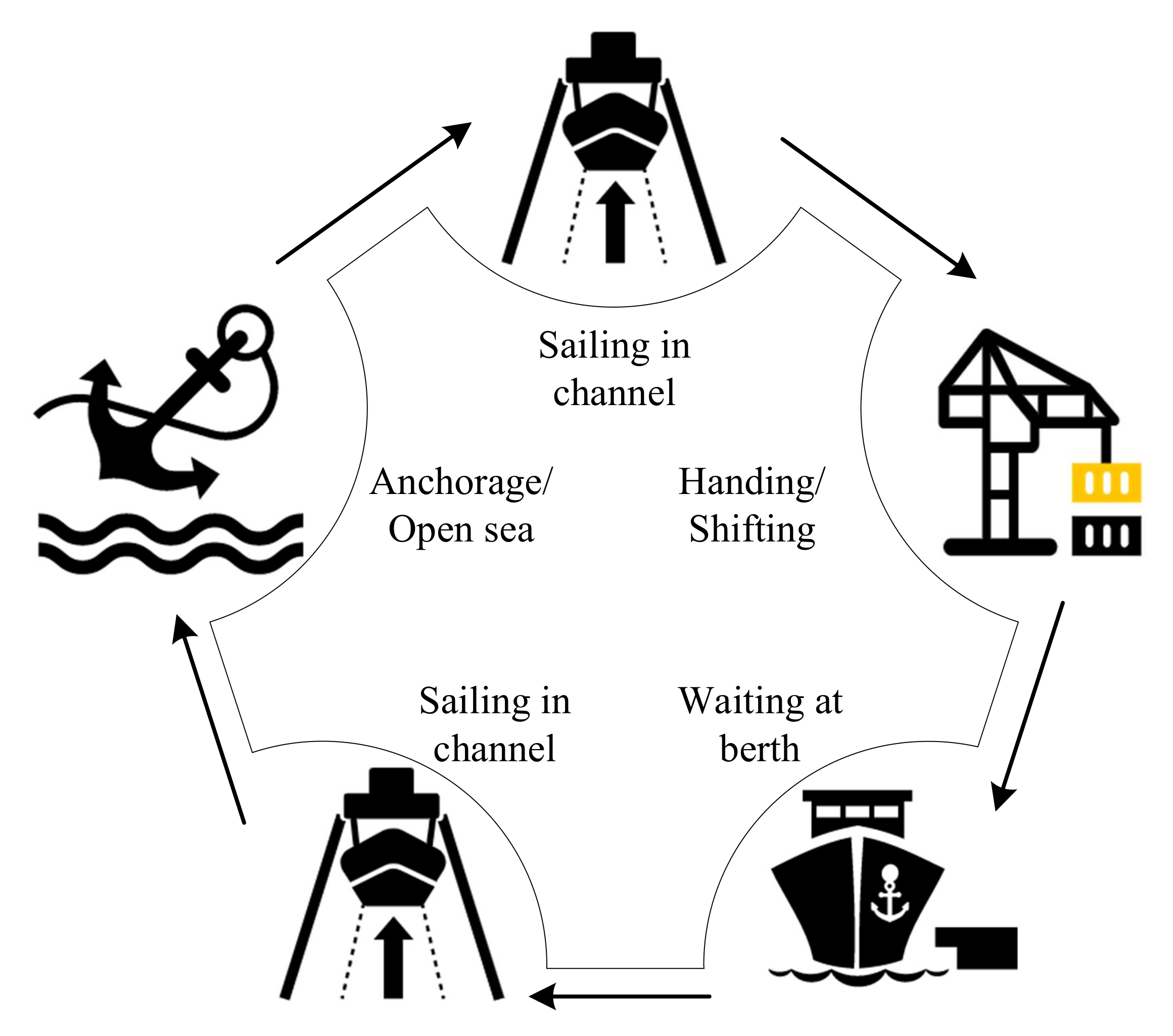
Figure 1 shows the simplified process of ship dispatching operations. From the figure, it can be observed that ship dispatching involves different environments, departments, and personnel. That is, the current port ship dispatching is a work handled by multiple departments. Each operation process between this kind of dispatch involves a more or less declaration process. For example, when one ship arrives near the port, it needs to report to the port management agency to apply for the next port operation. If the declaration process is appropriately simplified, and without considering berth allocation, pilotage management, and tugboat allocation, the operation process of ships entry and exit the port can be expressed as five parts, including the anchorage or waiting stage in the port, the sailing stage in the channel, and the loading and unloading stage. When optimizing and solving the ship scheduling problem, it is necessary to combine ship operation plans, navigation rules, safety guidelines, and port water environment to determine the ship’s entry and exit sequence and the corresponding assigned time.

In the process of using heuristic algorithms to solve the ship scheduling problem, the time parameters involved mainly include ETA, TSS, TES, NTW, schedule time window (TWS), safe interval, and sailing time (ST). Since the process of sea voyage will be cross-influenced by people (the subjective initiative of pilots and engineers onboard), machinery (ship performance), and environment (wind, waves, currents, rain, snow, fog), therefore, most of the time parameters mentioned above are all uncertain. Among them, ETA and ST are the main concern in dispatching. Due to the non-uniformity of sailing speed, the voyage time through the channel can be considered as an uncertain time parameter. As shown in the study [24], the speed distribution of ships entering and leaving the port in the channel of Tianjin Port on a certain day is uneven. Therefore, it is unreasonable for ships entering and exiting the port with a unified upward speed or downward speed for optimization.

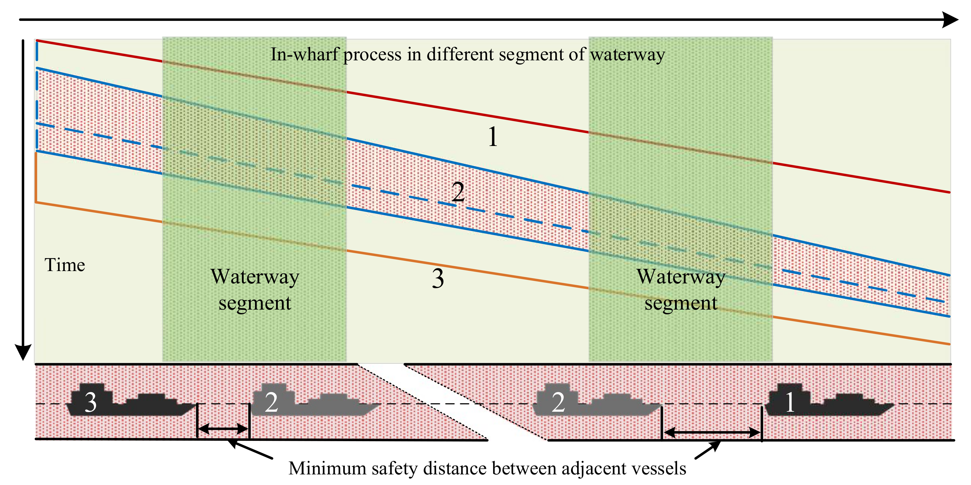
Besides, it is inappropriate for each ship to adopt a certain constant speed for dispatching and deduction, and it cannot meet the actual demand. To tackle this problem shown in Figure 2, this article mainly studies the uncertainty of the transit time caused by the unfixed speed of the ship when crossing the channel. Figure 2 is a simplified distance-time sketch of a vessel when passing through different segments of the waterway, in which the gray vessel (No. 2) passes through each segment of the waterway at an indeterminate speed. And, it also can be found from Figure 2, to keep the minimum safety distance, the delay time and the feasible time for entering the waterway of the next adjacent vessel (No. 3) would be affected by vessel 2. Therefore, it needs some calculation operations for time parameters between fuzzy numbers. Regard as the operations on fuzzy numbers, it is described in Section 3.3.

3.2. Tidal Impact

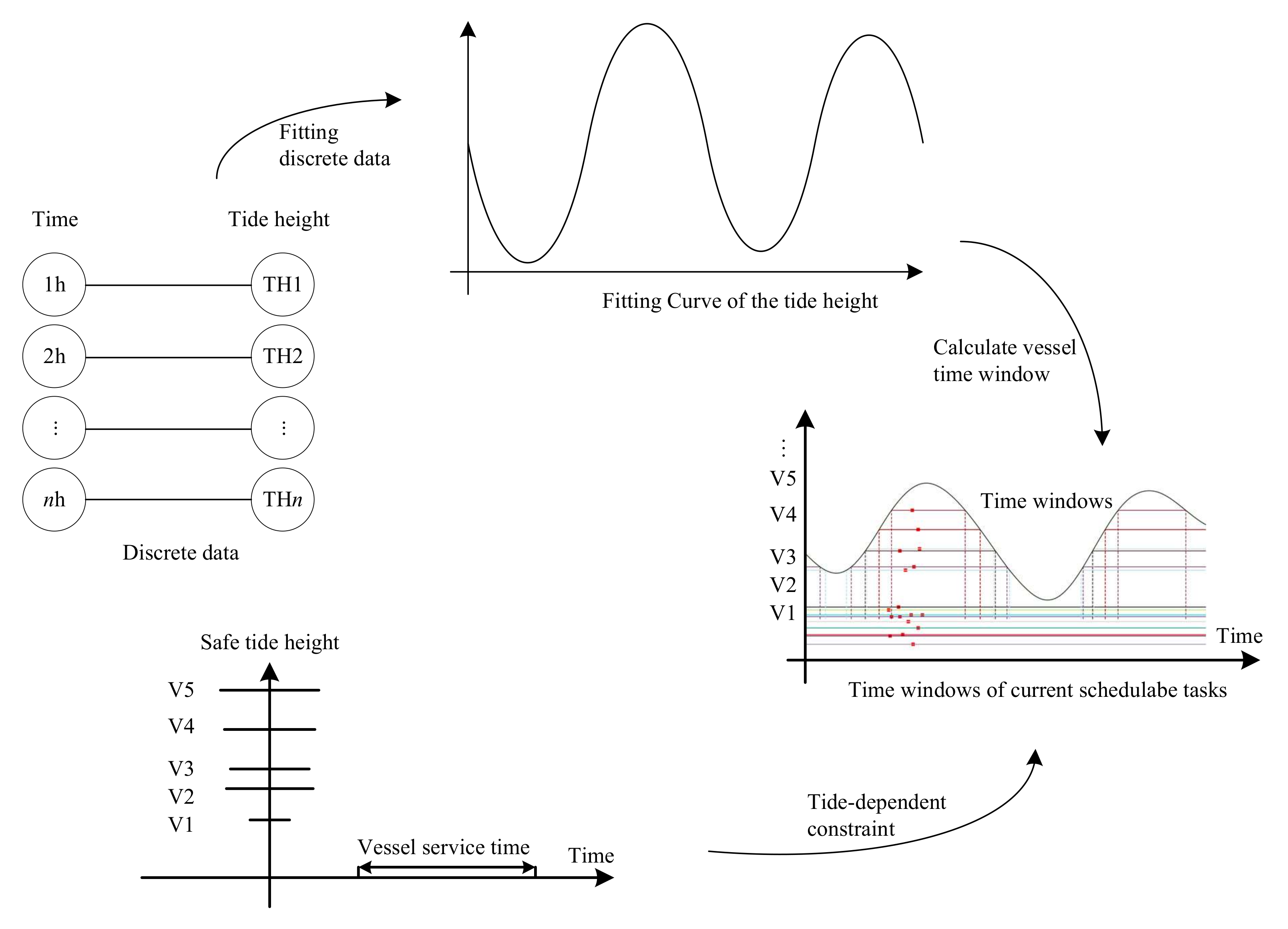
In the past two decades, the dead-weight tonnages of ships have increased exceed 4.3% [11]. However, the rapid development of the tonnage of ships has posed a great challenge to the scheduling of ports. Due to the existence of various variables such as ship tonnage, size, ship type, cargo capacity, consumption, etc., the ship’s draft has temporal and spatial attributes, and the draft refers to the distance between the ship’s waterline and the ship’s keel. In addition, the water depth of the channel in most ports is not sufficient for the safe entry and exit of all ships. To reduce the risk of deep-draft ships running aground in the channel, sufficient UKC should be reserved for navigation in port channels with limited draught. Different ports have different requirements for UKC, therefore, regard as tide-dependent vessels, the depth of the channel needs to be considered for the entering and exiting operation. In the previous studies, Zhang Bin [26,27] established the link between the draft of ships and the tidal height which can be calculated by the fitting curve of the tide height. Due to the existence of function solution constraints, a large number of calculations are required in the process of optimizing the solution of the ship scheduling model. Therefore, the model efficiency is low and it is difficult to meet the real-time requirements. Hence, instead of real-time calculation of tide height by determining the ship’s tide time window in advance. The procedure for determining the feasible tidal time windows is shown in Figure 3. Firstly, fit the quadratic polynomial between the adjacent 3 points of the tide height data shown in [24] so that the curve passes through all the points. After obtained the functional expression, the solution under each monotonic interval of tidal height needed to be solved by dichotomy, then the feasible tidal time window of each interval is determined, and finally, the time window can be determined after the multiple time windows are merged with Algorithm 1.

Algorithm 1: Determine vessel time windows.

3.3. Operations on Fuzzy Speed

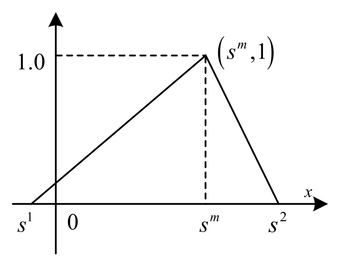
In the process of solving the fuzzy vessel scheduling problem, the operation of the fuzzy number is the key. The triangular fuzzy number (TFN) was utilized in the following studies for making a management decision. In this study, the fuzzy speed or the fuzzy sailing time can be shown as a TFN $\tilde{s}=(s^1,s^m,s^2)$ in Figure 4, where $[s^1,s^2]$ is the support interval, $(s^m,1)$ is the peak value. When $s^m$ is equal to half of the sum of $s^1$ and $s^2$, the triangular fuzzy number is the central fuzzy number.

When determining the ship’s entry and exit time, the fuzzy numbers need to be added together; when the ship’s end time is determined, the fuzzy numbers need to be summed; when comparing the fitness of the plan, the fuzzy numbers need to be compared. For triangular fuzzy numbers, the specific calculation method is as follows.

The addition operation between TFNs is mainly used to calculate the completion time of the vessel plan. The calculation method is shown in Equation (1), that is, the corresponding real number addition operation is performed on the ternary numbers of the two TFNs. Among them, ⊕ represents the fuzzy addition operator, and $\tilde{s},\tilde{t}$ respectively represent different TFNs.

$$\tilde{s}\oplus \tilde{t}=(s^1,s^2,s^3)+(t^1,t^2,t^3)=(s^1+t^1,s^2+t^2,s^3+t^3)$$

(1)

When comparing two fuzzy numbers, if both fuzzy numbers are triangular fuzzy numbers, the following three criteria can be used.

$$\left\{\begin{array}{c}\hfill c_1\left({\tilde{t}}_{i,w}\right)=\frac{t_{i,w}^1+t_{i,w}^2+t_{i,w}^3}{4}\\ \hfill c_2\left({\tilde{t}}_{i,w}\right)=t_{i,w}^2\\ \hfill c_3\left({\tilde{t}}_{i,w}\right)=t_{i,w}^3-t_{i,w}^1\end{array}i\in {\mathbb{V}}_m,\forall w\in \mathbb{W}.\right.$$

(2)

where the fuzzy number is set as ${\tilde{t}}_{i,w}=(t_{i,w}^1,t_{i,w}^2,t_{i,w}^3)$, which is the type of fuzzy sailing time in the mathematical model of vessel scheduling under uncertainty speed.

Comparing two TFNs ${\tilde{t}}_{i,w},{\tilde{t}}_{j,w}$ need using criteria $c_r\left({\tilde{t}}_{i,w}\right),r\in 1,2,3$ as shown in Equation (2). The first step is the comparison between $c_1\left({\tilde{t}}_{i,w}\right)$ and $c_1\left({\tilde{t}}_{j,w}\right)$, if $c_1\left({\tilde{t}}_{i,w}\right)>(<)c_1\left({\tilde{t}}_{j,w}\right)$, then ${\tilde{t}}_{i,w}>(<){\tilde{t}}_{j,w}$. If the first step is not satisfied, that is when $c_1\left({\tilde{t}}_{i,w}\right)\equiv c_1\left({\tilde{t}}_{j,w}\right)$ then continue the second step of comparison. If $c_2\left({\tilde{t}}_{i,w}\right)>(<)c_2\left({\tilde{t}}_{j,w}\right)$, then ${\tilde{t}}_{i,w}>(<){\tilde{t}}_{j,w}$. If the first two steps fail to compare, then continue the third step based on the comparison between $c_3\left({\tilde{t}}_{i,w}\right)$ and $c_3\left({\tilde{t}}_{j,w}\right)$, If $c_3\left({\tilde{t}}_{i,w}\right)>(<)c_3\left({\tilde{t}}_{j,w}\right)$, then ${\tilde{t}}_{i,w}>(<){\tilde{t}}_{j,w}$.

4. Integrated Model for Vessel Scheduling with Fuzzy Speed

The port decision-maker cannot obtain the accurate channel occupation time of each ship during the actual sailing process in the planning stage of the ship’s initial entry and exit plan. Therefore, it is necessary to give each ship an estimated speed based on experience. This article assumes that the ship’s sailing speed in the channel is a fuzzy value is called fuzzy speed. At the same time, the port and channel resources are fixed, and the same channel resource may be occupied by multiple ships, so the available time of the channel resources of each ship also becomes an estimated fuzzy value. It is precise because of the uncertainty of this external factor that the ship’s original plan is inaccurate. Therefore, during the execution of the plan, the original plan may be revised many times, which may result in increased costs and reduced navigation efficiency in port waters. At the same time, some ships may not be able to complete related operations on time. This requires port decision-makers in the project planning stage to reasonably arrange the front and back logical constraints of each ship, and minimize the ship completion time as the primary performance indicator for dispatch.

4.1. Model Assumptions and Notations

In practice, when a ship is preparing to enter, depart, or shift berths, they need to communicate with the port or the ship traffic service center of the maritime administrative department on the corresponding VHF channel according to the port area in which they are located. After comprehensively considering the port traffic distribution, channel hydrology and meteorology, and the use of anchorages and berths, the start time of the port entry, exit, or relocation operation is finally determined. Taking into account the actual situation of port production and the incompleteness of the model, a series of assumptions are defined as follows:

• All ships can complete relevant preparations before the planned time of entry and exit;
• The anchorage capacity and berth conditions have no impact on the arrangement of the ship’s entry and exit plans;
• Ships in the channel entry and exit in order, no overtaking is allowed, and non-scheduled ships will not affect the operation of the dispatched ships;
• Except for the restricted draft of some ships, there are no special requirements for the navigation environment.

The sets and parameters is shown in

Table 1. Notation.

Sets and Parameters
Notations:
$\mathbb{V}$: the set of vessels
$\mathbb{M}$: the set of movement types
$\mathbb{W}$: the set of waterways
$i,j$: the index of vessel
m: the index of movement types, $m=1,2$. 1 inbound vessel; 2 outbound vessel
w: the segment of waterways
$ET{A}_{i,w}$: the estimated time of arrival for the vessel $i,i\in {\mathbb{V}}_m$ in the segment w
$L_w$: the length of the segment w
${\widetilde{TES}}_{i,w}$: the time when the vessel $i,i\in {\mathbb{V}}_m$ exit the segment w of waterway
${\widetilde{TSS}}_{i,w}$: the time when the vessel $i,i\in {\mathbb{V}}_m$ enter the segment w of waterway, that is, the allocated time
${\widetilde{TCS}}_{i,w}$: the time of traffic control for the vessel $i,i\in {\mathbb{V}}_m$ in the segment w
${\tilde{t}}_{i,w}$: voyage time for vessel $i,i\in {\mathbb{V}}_m$ through the segment w
${{\widetilde{TW}}^r}_i$: right boundary of the feasible tidal time window for the vessel $i,i\in {\mathbb{V}}_m$
${{\widetilde{TW}}^l}_i$: left boundary of the feasible tidal time window for the vessel $i,i\in {\mathbb{V}}_m$
$t_1$: safe separation between ships of the same type of movement
$t_2$: safe separation between ships of different types of movement
$\mathcal{C}$: a positive integer that is sufficiently large
Decision variables:
$\Gamma$: the makespan of all vessels waiting to enter and exit the port
${\widetilde{TSS}}_{i,w}$: the time when the vessel $i,i\in {\mathbb{V}}_m$ enter the segment w of waterway
$B_{m,i,j}$: binary, equal to 1 if ship $i,i\in {\mathbb{V}}_m$ falls behind ship $j,j\in {\mathbb{V}}_m$, and 0 otherwise
$I_{i,j}$: binary, equal to 1 if ship $i,i\in {\mathbb{V}}_m$ falls behind ship $j,j\in {\mathbb{V}}_m$, and 0 otherwise

.

4.2. Mathematical Model

Objective

$$min\Gamma =\underset{i\in \mathbb{V}}{max}({\widetilde{TSS}}_{i,0}\oplus \sum _{w\in \mathbb{W}}{\tilde{t}}_{i,w}),\mathbb{V}=\underset{m\in \mathbb{M}}{\cup }{\mathbb{V}}_m$$

(3)

Subject to

$${\widetilde{TCS}}_{i,w}\ominus {\widetilde{TSS}}_{i,w}\le 0,\forall i\in {\mathbb{V}}_m,\forall w\in \mathbb{W}$$

(4)

$${\widetilde{ETA}}_i\ominus {\widetilde{TSS}}_{i,0}\le 0,\forall i\in {\mathbb{V}}_m$$

(5)

$${\widetilde{TES}}_{i,w}={\widetilde{TSS}}_{i,w}\oplus \sum _{w\in \mathbb{W}}{\tilde{t}}_{i,w},\forall i\in {\mathbb{V}}_m,\forall w\in \mathbb{W}$$

(6)

$${{\widetilde{TW}}^l}_i\ominus {\widetilde{TSS}}_{i,w}\le 0,\forall i\in {\mathbb{V}}_m,\forall w\in \mathbb{W}$$

(7)

$${\widetilde{TSS}}_{i,0}\oplus \mathsf{\Sigma }{\tilde{t}}_{i,w}\ominus {{\widetilde{TW}}^r}_i\le 0,\forall i\in {\mathbb{V}}_m,\forall w\in \mathbb{W}$$

(8)

$${\tilde{t}}_{i,w}=L_w÷{\tilde{V}}_{i,w},\forall i\in {\mathbb{V}}_m,\forall w\in \mathbb{W}$$

(9)

$${\widetilde{TSS}}_{i,w+1}={\widetilde{TSS}}_{i,w}+{\tilde{t}}_{i,w},\forall i\in {\mathbb{V}}_m,\forall w\in \mathbb{W}$$

(10)

$$|{\widetilde{TSS}}_{i,w}\ominus {\widetilde{TSS}}_{j,w}|\ge t_1,\forall i,j\in {\mathbb{V}}_m,\forall w\in \mathbb{W},i\ne j$$

(11)

$$|{\widetilde{TES}}_{i,w}\ominus {\widetilde{TES}}_{j,w}|\ge t_1,\forall i,j\in {\mathbb{V}}_m,\forall w\in \mathbb{W},i\ne j$$

(12)

$$({\widetilde{TSS}}_{i,w}\ominus {\widetilde{TSS}}_{j,w})\times ({\widetilde{TES}}_{i,w}\ominus {\widetilde{TES}}_{j,w})\ge 0,\forall i,j\in {\mathbb{V}}_m,\forall w\in \mathbb{W},i\ne j$$

(13)

$$\left\{\begin{array}{c}\hfill {\widetilde{TSS}}_{1,i,w}\ominus {\widetilde{TES}}_{2,j,w}\ge t_2,if{I}_{i,j}=1\\ \hfill {\widetilde{TSS}}_{2,j,w}\ominus {\widetilde{TES}}_{1,i,w}\ge t_2,if{I}_{i,j}=0\end{array}\forall i\in {\mathbb{V}}_1,\forall j\in {\mathbb{V}}_2,\forall w\in \mathbb{W}.\right.$$

(14)

In this study, the mathematical model aims to minimize the time for the last ship to cross the channel. The specific calculation method is shown in Equation (3). Constrained by the time window of the port traffic organization, the constraint relationship between the allocation time for one vessel and the traffic control time is defined, as shown in Equation (4). Equation (5) can ensure that the allocated time of one ship must be later than the estimated time of arrival of the ship. The time for one vessel exit channel can be obtained by the fuzzy addition between the fuzzy sailing time and the fuzzy allocated time of the vessel, as shown in Equation (6). With regard to tide-dependent vessels, Equations (7) and (8) are defined to ensure that they always meet the requirements of safe water depth during navigation. Equation (7) describes the relationship between the ship’s entry time to the channel and the minimum value of the feasible tidal time window. Equation (8) describes the relationship between the ship’s exit time and the maximum value of the feasible tidal time window. Equation (9) states the ambiguous voyage time of one vessel in different segments of one waterway. The time relationship between vessels’ entry and exit adjacent segments of one waterway is defined as shown in Equation (10). Equations (11) and (12) respectively describe the safety interval that any two vessels with the same movement type should satisfy when entering and leaving the same segment of a waterway, where the safety interval is represented by the sailing time $t_1$. Equation (13) can ensure that two vessels with the same movement type will not overtake in any segment of a waterway. Two vessels with different types of movement should satisfy the constraints as described in Equation (14) when entering or exiting the same segment of a waterway.

Due to the existence of nonlinear constraints in the above equations, and nonlinear constraint problems are difficult to optimize. Therefore, in order to further simplify the mathematical model, binary $B_{m,i,j}$ was introduced to transform Equations (11) and (12) into Equations (15) and (16).

$$\left\{\begin{array}{c}\hfill {\widetilde{TSS}}_{m,i,w}\ominus {\widetilde{TSS}}_{m,j,w}\ge t_1,if B_{m,i,j}=1\\ \hfill {\widetilde{TSS}}_{m,j,w}\ominus {\widetilde{TSS}}_{m,i,w}\ge t_1,if B_{m,i,j}=0\end{array}\forall i,j\in {\mathbb{V}}_m,\forall w\in \mathbb{W},i\ne j.\right.$$

(15)

$$\left\{\begin{array}{c}\hfill {\widetilde{TES}}_{m,i,w}\ominus {\widetilde{TES}}_{m,j,w}\ge t_1,if B_{m,i,j}=1\\ \hfill {\widetilde{TES}}_{m,j,w}\ominus {\widetilde{TES}}_{m,i,w}\ge t_1,if B_{m,i,j}=0\end{array}\forall i,j\in {\mathbb{V}}_m,\forall w\in \mathbb{W},i\ne j.\right.$$

(16)

Equations (15) and (16) can be further expressed as Equations (17)–(20) by introducing a sufficiently large positive constant $\mathcal{C}$.

$$B_{m,i,j}\times \mathcal{C}+{\widetilde{TSS}}_{m,j,w}\ominus {\widetilde{TSS}}_{m,i,w}\ge t_1,\forall i,j\in {\mathbb{V}}_m,\forall w\in \mathbb{W},i\ne j.$$

(17)

$$(1-B_{m,i,j}\times \mathcal{C})+{\widetilde{TSS}}_{m,i,w}\ominus {\widetilde{TSS}}_{m,j,w}\ge t_1,\forall i,j\in {\mathbb{V}}_m,\forall w\in \mathbb{W},i\ne j.$$

(18)

$$B_{m,i,j}\times \mathcal{C}+{\widetilde{TES}}_{m,j,w}\ominus {\widetilde{TES}}_{m,i,w}\ge t_1,\forall i,j\in {\mathbb{V}}_m,\forall w\in \mathbb{W},i\ne j.$$

(19)

$$(1-B_{m,i,j}\times \mathcal{C})+{\widetilde{TES}}_{m,i,w}\ominus {\widetilde{TES}}_{m,j,w}\ge t_1,\forall i,j\in {\mathbb{V}}_m,\forall w\in \mathbb{W},i\ne j.$$

(20)

In the same way, Equation (14) can also be transformed into Equations (21) and (22) by introducing $\mathcal{C}$ mentioned above.

$$I_{i,j}\times \mathcal{C}+{\widetilde{TSS}}_{2,j,w}\ominus {\widetilde{TES}}_{1,i,w}\ge t_2,\forall i\in {\mathbb{V}}_1,j\in {\mathbb{V}}_2,\forall w\in \mathbb{W}.$$

(21)

$$(1-I_{i,j}\times \mathcal{C})+{\widetilde{TSS}}_{1,i,w}\ominus {\widetilde{TES}}_{2,j,w}\ge t_2,\forall i\in {\mathbb{V}}_1,j\in {\mathbb{V}}_2,\forall w\in \mathbb{W}.$$

(22)

5. GA for FVSP with Uncertain Speed

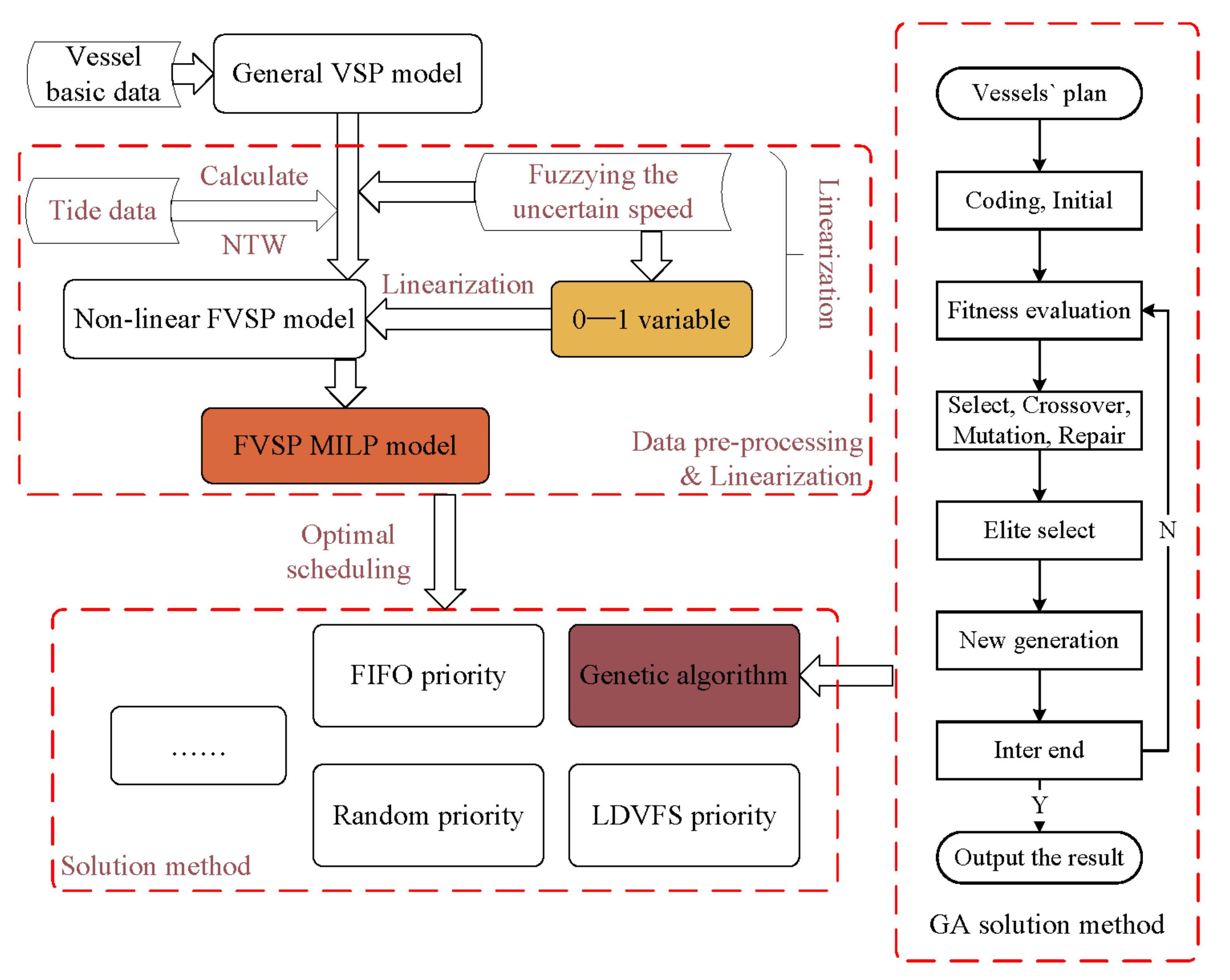
To solve VSP with uncertainty time, there exist many methods that can be used, e.g., heuristic algorithm (GA, TS, CS, and CG, et al.), Lagrange multiplier methods, gradient descent, and quasi–newton methods, et al. Considering that the genetic algorithm has good global search capabilities, it can quickly search for all solutions in the solution space without falling into the trap of a rapid decline in locally optimal solutions, and it can also use inherent parallelism to conveniently perform distributed calculations to improve optimization efficiency; therefore, in this study, the authors utilized a heuristic algorithm (GA) to solve the scheduling optimization problem. The process of the designed genetic algorithm for tackling the FVSP involves coding, similarity calculation, population initialization, fitness evaluation, selection, crossover, mutation, and elite selection as shown in Figure 5. The framework of optimal scheduling with uncertain speed includes three parts. One is data pre–processing and the construction of the MILP model, the second is the design of GA–based heuristic solution method, and the third is the comparative analysis of optimization. Compared with the general vessel scheduling flowchart, the improvements of the FVSP mode can be reflected in two aspects. One is that the fitness evaluation is based on TFN, and the second one is the addition of data pre–processing and linearization stages.

5.1. Coding and Initialization

In this study, we adopt single-layer coding to represent an individual with a real number sequence. The chromosome elements were formatted with an array structure. Each array structure represents an individual, and all individuals randomly generated make up the initial population. The integer number sequence expresses the vessel sequence. For N vessels, each vessel is indexed as a unique integer from 1 to N. For example, $p=(1,3,8,9,2,10,6,5,7,4)$ is a chromosome that represents a scheduling sequence (solution) of the corresponding vessel, where the first one would be scheduled is vessel 1, the next one is vessel 3, and the last one is vessel 4. In the same way, the population can be generated that consists of many individuals generated randomly as a vector $Pop={[p_1,p_2,\cdots ,p_n]}^{\top }$.

5.2. Crossover, Mutation, and Selection

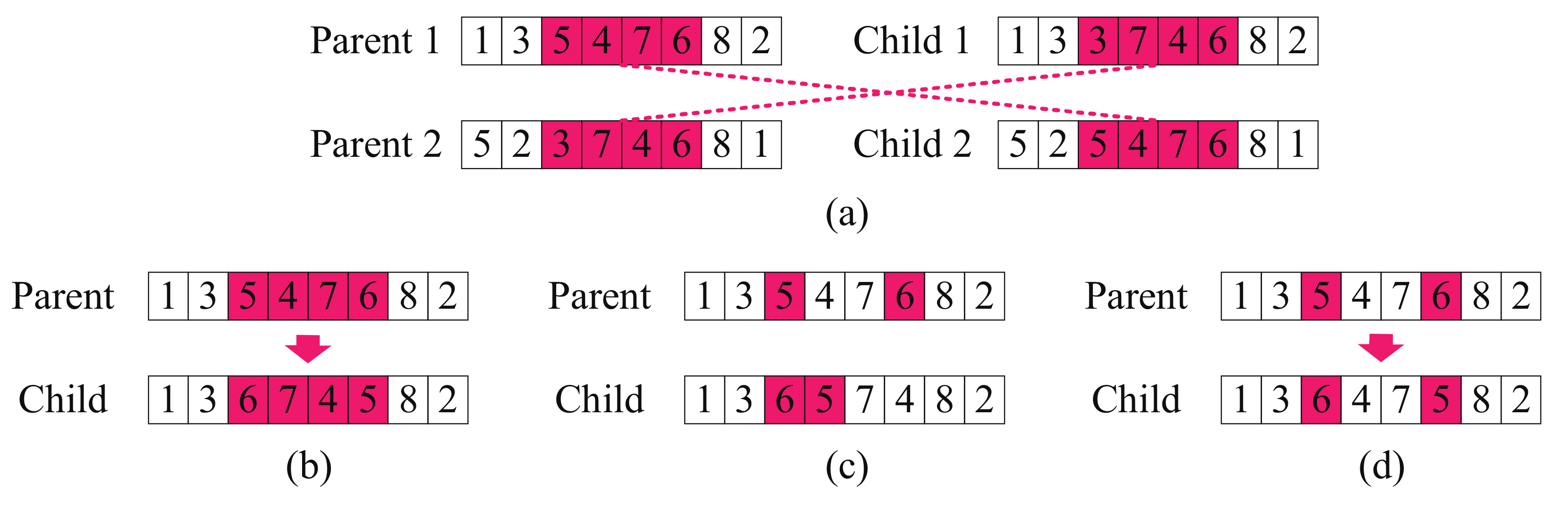
In this study, the partial-mapped crossover (PMX) is used in the GA. The first step randomly chooses a few adjacent genes at the same position from two individuals (parent 1 and parent 2). The second step, swap the positions of the two gene segments. The last step, map the conflicting genes and then obtain the conflict-free offspring genes. In terms of mutation operation, local reversal mutation, swap mutation, and insert mutation are all applied to this study, as shown in Figure 6. The specific operation is that we randomly select one of the above three methods to perform mutation operations on the population during the iterative process. The elite selection is used to select the best top from the union of parent and offspring after crossover operation and mutation operation.

5.3. Illegal Solution

The population generation in the genetic algorithm generally adopts the method of random generation, so infeasible solutions that violate the constraint conditions will appear. At the same time, feasible solutions may also produce infeasible solutions after genetic operators’ cross-mutation and other operations. At present, the commonly used processing methods can be divided into the following four categories, discarding infeasible solutions, repairing infeasible solutions, improving genetic operators, and penalty functions. In this study, a penalty function is adopted to tackle the infeasible solution problem as Equation (23). For an infeasible solution, a certain penalty is imposed, so that the objective function value becomes a larger value while the solution is illegal. This method can properly accept infeasible solutions, expand the search space, and make the infeasible solutions possible, to retain the excellent genes. After continuous iteration, the population will gradually converge to the feasible solution.

$$\Gamma =\mathcal{C}+\underset{i\in \mathbb{V}}{max}({\widetilde{TSS}}_{i,0}\oplus \sum _{w\in \mathbb{W}}{\tilde{t}}_{i,w}),\mathbb{V}=\underset{m\in \mathbb{M}}{\cup }{\mathbb{V}}_m$$

(23)

where $\mathcal{C}$ is a large value, and 1000 is used in this study. If the population is illegal, the fitness value becomes a larger value, otherwise, it remains unchanged.

The stopping criterion utilized in this solution method is met if there has been a certain number of consecutive generations without improvement of the best-known individual of the population or a certain total number of generations has been reached.

6. Computational Experiments

The parameters of the simulation waterway are as follows: the waterway length and depth are 12,964 m, and 12.5 m, respectively. Regarding the parameter setting of the heuristic algorithm GA, we set the number of individuals in the population to the number of ships in different cases; population size is 10; mutation probability is 0.8; the termination criterion includes a maximum number of iterations which was set as 2000, and the number of times that the minimum fitness value remained unchanged in the two adjacent iterations, which was set as 300; sufficiently large positive constant is 1000.

6.1. Simulation Setting

Considering the estimated time of arrival, feasible tidal time windows, and some constraints of the environment, we processed 13 case studies in the next section.

In this section, we present the cases to analyze the comparison experiments which include abbreviation and combination index of vessels. The case of different sizes for comparison are randomly combined based on the data listed in

Table 2. Vessel static application information.

Vessel No.	Speed (m/s)	FST	ETA	Draft (m)	UKC (m)
1	(8.0, 6.3, 4.96)	(0.9, 1.1, 1.4)	5:00:00	11.50	1.42
2	(5.2, 4.09, 3.22)	(1.3, 1.7, 2.2)	5:05:00	11.30	1.00
3	(8.7, 6.85, 5.39)	(0.8, 1.0, 1.3)	5:10:00	10.70	2.06
4	(8.0, 6.3, 4.96)	(0.9, 1.1, 1.4)	5:10:00	9.80	0.92
5	(5.8, 4.57, 3.6)	(1.2, 1.5, 1.9)	5:15:00	10.90	0.94
6	(6.5, 5.12, 4.03)	(1.1, 1.4, 1.8)	5:35:00	10.90	2.09
7	(8.9, 7.01, 5.52)	(0.8, 1.0, 1.3)	5:40:00	11.80	0.96
8	(6.8, 5.35, 4.21)	(1.0, 1.3, 1.7)	5:40:00	14.20	0.13
9	(7.7, 6.06, 4.77)	(0.9, 1.1, 1.4)	5:50:00	10.80	0.73
10	(7.0, 5.51, 4.34)	(1.0, 1.3, 1.7)	5:50:00	12.20	0.13
11	(8.1, 6.38, 5.02)	(0.9, 1.1, 1.4)	6:00:00	11.90	1.97
12	(8.5, 6.69, 5.27)	(0.8, 1.0, 1.3)	6:10:00	9.90	2.74
13	(7.4, 5.83, 4.59)	(0.9, 1.1, 1.4)	6:10:00	9.30	2.46
14	(7.7, 6.06, 4.77)	(0.9, 1.1, 1.4)	6:20:00	9.90	2.90
15	(6.8, 5.35, 4.21)	(1.0, 1.3, 1.7)	6:24:00	10.00	1.22
16	(8.6, 6.77, 5.33)	(0.8, 1.0, 1.3)	6:24:00	13.30	2.00
17	(7.2, 5.67, 4.46)	(1.0, 1.3, 1.7)	6:27:00	11.50	0.60
18	(7.6, 5.98, 4.71)	(0.9, 1.1, 1.4)	6:30:00	12.10	1.85
19	(7.9, 6.22, 4.9)	(0.9, 1.1, 1.4)	6:30:00	10.80	0.92
20	(6.7, 5.28, 4.16)	(1.0, 1.3, 1.7)	6:33:00	10.40	1.02
21	(5.1, 4.02, 3.17)	(1.4, 1.8, 2.3)	6:40:00	9.50	1.45
22	(7.7, 6.06, 4.77)	(0.9, 1.1, 1.4)	6:45:00	12.90	1.94
23	(5.5, 4.33, 3.41)	(1.3, 1.7, 2.2)	6:45:00	11.60	0.89
24	(7.1, 5.59, 4.4)	(1.0, 1.3, 1.7)	6:50:00	12.50	1.88
25	(7.7, 6.06, 4.77)	(0.9, 1.1, 1.4)	7:00:00	12.00	0.80

. Each case was generated with the combination of ship index as shown in

Table 3. Combination of case.

Case	Combination Index (Ship No.)
Case_10_1	22, 12, 3, 13, 23, 11, 5, 2, 18, 10
Case_10_2	8, 13, 1, 2, 19, 6, 3, 12, 11, 16
Case_10_3	2, 21, 14, 12, 5, 17, 19, 22, 10, 6
Case_10_4	4, 18, 3, 1, 20, 9, 14, 12, 15, 10
Case_15_1	6, 3, 5, 25, 18, 16, 2, 9, 13, 12, 20, 24, 8, 10, 17
Case_15_2	20, 22, 12, 17, 1, 5, 16, 25, 3, 4, 15, 9, 23, 24, 11
Case_15_3	22, 7, 16, 4, 2, 13, 18, 17, 15, 9, 1, 24, 8, 3, 20
Case_15_4	22, 14, 6, 1, 25, 2, 19, 20, 21, 23, 24, 10, 3, 17, 9
Case_20_1	2, 22, 7, 11, 20, 5, 19, 9, 17, 12, 14, 1, 3, 23, 24, 6, 8, 16, 13, 4
Case_20_2	24, 4, 9, 21, 7, 25, 6, 13, 15, 3, 12, 19, 1, 18, 2, 11, 14, 17, 20, 5
Case_20_3	15, 14, 19, 1, 8, 6, 9, 5, 4, 24, 13, 10, 16, 22, 11, 7, 21, 3, 17, 25
Case_20_4	22, 11, 17, 24, 5, 3, 16, 14, 20, 6, 7, 9, 13, 12, 18, 2, 8, 25, 19, 1
Case_25_1	9, 13, 6, 23, 8, 4, 17, 22, 19, 21, 3, 15, 7, 20, 2, 16, 24, 10, 11, 12, 25, 14, 5, 18, 1

. Four groups are generated for each length of case and they are present by the sign ‘Case_X_Y’. For example, ‘Case_10_1’ is case 1 of length 10.

6.2. Data Preprocessing

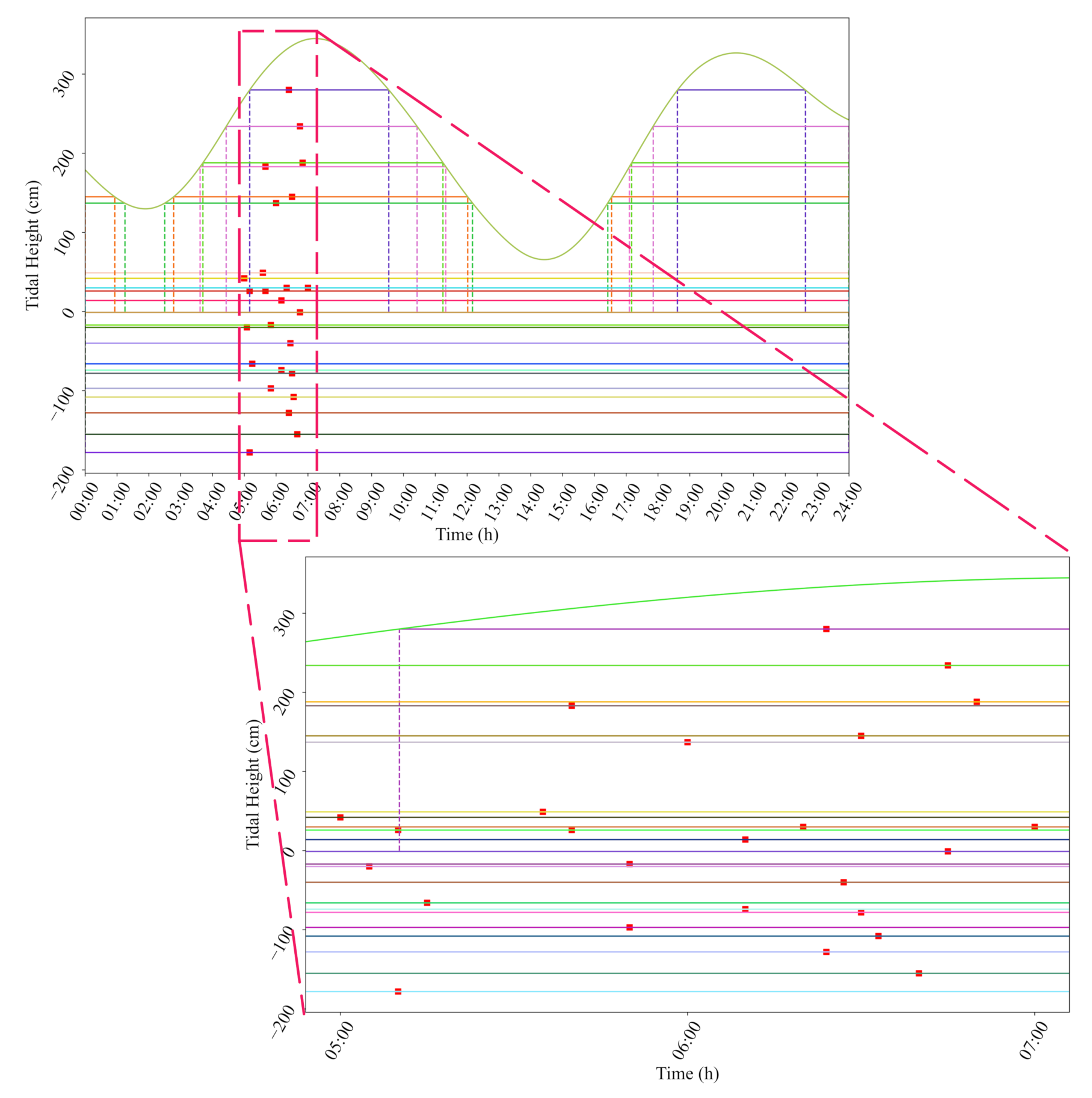
Figure 7 and

Table 4. Feasible tidal time windows for tide-dependent vessels.

Ship No.	FTTW (H)
8	((3.61, 11.33), (17.1, 24.0))
11	((0, 1.25), (2.5, 12.17), (16.42, 24.0))
16	((5.17, 9.54), (18.61, 22.63))
18	((0, 0.93), (2.78, 12.02), (16.54, 24.0))
22	((4.43, 10.43), (17.85, 24.0))
24	((3.7, 11.24), (17.17, 24.0))

are the results computed by the Algorithm 1 for determining feasible tidal time windows of each vessel in Table 2 based on the tide data in [24], which shows that the waterway depth at each vessel’s feasible tidal time window is greater than the requirement for safe navigation with a safe UKC while the vessel is proceeding in shallow waterway. From the Figure 7, due to the characteristics of the fitted tide curve, we can observe that there are several ships with multiple feasible tidal time windows. Regarding a tide-depend vessel, if it has multiple FTTWs, it is necessary to ensure that it can successfully pass the channel under the assigned tide cycle during the sequence arrangement.

6.3. Comparison and Discussion

6.3.1. Comparison under the Priority-Based Scheduling Methods

In this section, some scheduling rules are used to compare and analyze the optimal results. These priority rules include first–in–first–out (FIFO), larger draft vessel first service (LDVFS), and random service (RS) [24]. Under the FIFO scheduling rules, the arrival time of ships will be utilized as the basis for determining the sequence of entry and exit, that is, the ship arriving at the port earlier can enter the channel earlier, and otherwise, the ship will enter the channel later. Under the LDVFS scheduling rules, the draft of ships will be utilized as the basis for the sequence of entry and exit. Under the same conditions, tide-dependent ships have the priority of entry and exit. The random dispatch rule is the same as its literal meaning, the order assigned for all ships is set randomly.

Table 5. Comparison among the different scheduling rules (Case_25_1).

Mode	Vessel Scheduling Order	Makespan
FIFO	25, 15, 11, 6, 23, 3, 13, 5, 1, 18, 19, 2, 20, 22, 16, 12, 7, 24, 9, 14, 10, 4, 8, 17, 21	–
LDVFS	16, 8, 17, 5, 24, 19, 3, 25, 22, 21, 13, 11, 20, 4, 18, 15, 7, 23, 2, 9, 1, 14, 12, 10, 6	(11.75, 12.65, 13.65)
RS	5, 3, 16, 23, 19, 4, 24, 8, 10, 17, 20, 7, 9, 25, 6, 15, 22, 12, 14, 18, 2, 13, 21, 11, 1	(11.60, 12.70, 13.90)
GA	11, 6, 25, 3, 5, 18, 20, 13, 16, 24, 22, 19, 9, 1, 17, 7, 14, 23, 10, 15, 4, 12, 2, 21, 8	(9.38, 9.88, 10.48)

shows the results of different scheduling modes, including the scheduling sequence and makespan.

Table 6. Fuzzy vessel scheduling results (Case_25_1).

Ship No.	FST	Scheduled Order	TSS	TES
9	(0.9, 1.1, 1.4)	11	(5.17 5.17 5.17)	(5.97 6.17 6.47)
13	(0.9, 1.1, 1.4)	6	(5.27 5.27 5.27)	(6.17 6.37 6.67)
6	(1.1, 1.4, 1.8)	25	(5.37 5.37 5.37)	(6.27 6.47 6.77)
23	(1.3, 1.7, 2.2)	3	(5.58 5.58 5.58)	(6.68 6.98 7.38)
8	(1.0, 1.3, 1.7)	5	(5.78 5.78 5.78)	(6.78 7.08 7.48)
4	(0.9, 1.1, 1.4)	18	(5.88 5.88 5.88)	(6.88 7.18 7.58)
17	(1.0, 1.3, 1.7)	20	(6.18 6.28 6.38)	(6.98 7.28 7.68)
22	(0.9, 1.1, 1.4)	13	(6.28 6.38 6.48)	(7.08 7.38 7.78)
19	(0.9, 1.1, 1.4)	16	(6.38 6.48 6.58)	(7.18 7.48 7.88)
21	(1.4, 1.8, 2.3)	24	(6.48 6.58 6.68)	(7.38 7.68 8.08)
3	(0.8, 1.0, 1.3)	22	(6.58 6.68 6.78)	(7.48 7.78 8.18)
15	(1.0, 1.3, 1.7)	19	(6.68 6.78 6.88)	(7.58 7.88 8.28)
7	(0.8, 1.0, 1.3)	9	(6.78 6.88 6.98)	(7.68 7.98 8.38)
20	(1.0, 1.3, 1.7)	1	(6.88 6.98 7.08)	(7.78 8.08 8.48)
2	(1.0, 1.3, 1.7)	17	(6.98 7.08 7.18)	(7.98 8.38 8.88)
16	(0.8, 1.0, 1.7)	7	(7.08 7.18 7.28)	(8.08 8.48 8.98)
24	(1.0, 1.3, 1.7)	14	(7.18 7.28 7.38)	(8.18 8.58 9.08)
10	(1.0, 1.3, 1.7)	23	(7.28 7.38 7.48)	(8.48 8.88 9.38)
11	(0.9, 1.1, 1.4)	10	(7.38 7.48 7.58)	(8.78 9.28 9.88)
12	(0.8, 1.0, 1.3)	15	(7.58 7.68 7.78)	(8.88 9.38 9.98)
25	(0.9, 1.1, 1.4)	4	(7.68 7.78 7.88)	(8.98 9.48 10.08)
14	(0.9, 1.1, 1.4)	12	(8.08 8.28 8.48)	(9.08 9.58 10.18)
5	(1.2, 1.5, 1.9)	2	(8.28 8.58 8.88)	(9.18 9.68 10.28)
18	(0.9, 1.1, 1.4)	21	(8.38 8.68 8.98)	(9.28 9.78 10.38)
1	(0.9, 1.1, 14)	8	(8.48 8.78 9.08)	(9.38 9.88 10.48)

provided the certain fuzzy time including fuzzy sailing time, fuzzy start time, and fuzzy end time. In case ‘Case_25_1’, FIFO is mainly used as manual scheduling did not generate a scheduling sequence during a certain period. The result of GA is better than the other three scheduling methods. The lower bound of makespans calculated by LDVFS and RS are 11.75 and 11.60, respectively. These values are more than 23% higher than that for GA. The upper bound of makespans calculated by LDVFS and RS are 11.75 and 11.60, respectively. These values are more than 30% higher than that for GA. Therefore, the heuristic scheduling algorithm not only can avoid the illegal solution appearing in FIFO mode but also can improve vessel scheduling efficiency and traffic safety.

6.3.2. Comparison under Varying Problem Scales

Since the actual situation in a port is complex, to verify the applicability of the proposed FVSP model and algorithm on different problem scales in the actual situation, the method of simulation is utilized in the following experiments. The data is shown in Table 2, which simulates conditions in a one-way waterway affected by tidal height in Tianjin port, China. The arrival period is 5:00–7:00. Constrained by tidal height, the tide height data of Tianjin during one day are used. There are 25 vessels in total and divided into different scales for comparison experiments. To verify the effect of the proposed model, 25 vessels are divided into 13 cases as shown in Table 3. We carried out 13 groups of experiments with 10 vessels, 15 vessels, 20 vessels, and 25 vessels, respectively. All twelve case studies experimented at the condition where the number of times that the minimum fitness value remained unchanged in the two adjacent iterations was set as 300. The results (makespans) of different rules in each case are presented in

Table 7. Comparison of the results of different methods under different problem scales.

Case	GA	FIFO	LDVFS	RS	Min
Case_10_1	(8.15, 8.55, 9.05)	(8.18, 8.88, 9.68)	(9.35, 9.85, 10.45)	(9.85, 10.55, 11.35)	1
Case_10_2	(7.60, 7.80, 8.10)	(7.60, 8.10, 8.70)	(9.00, 9.60, 10.30)	(8.70, 9.20, 9.80)	1
Case_10_3	(8.27, 8.67, 9.17)	(8.25, 8.75, 9.35)	(9.95, 10.65, 11.45)	(9.07, 9.67, 10.37)	1
Case_10_4	(7.75, 8.05, 8.45)	(7.73, 8.23, 8.83)	(8.60, 9.00, 9.5)	(8.35, 8.85, 9.45)	1
Case_15_1	(8.07, 8.57, 9.17)	(8.58, 9.38, 10.28)	(10.13, 10.83, 11.63)	(9.90, 10.70, 11.60)	1
Case_15_2	(8.40, 8.80, 9.30)	(8.50, 9.00, 9.60)	(9.85, 10.45, 11.15)	(9.95, 10.65, 11.45)	1
Case_15_3	(8.20, 8.50, 8.90)	(8.30, 9.10, 10.00)	(9.65, 10.25, 10.95)	(9.93, 10.63, 11.43)	1
Case_15_4	(8.60, 9.00, 9.50)	(9.00, 10.0, 11.10)	(10.55, 11.35, 12.25)	(9.85, 10.55, 11.35)	1
Case_20_1	(8.80, 9.20, 9.70)	(9.60, 10.6, 11.70)	(10.55, 11.25, 12.05)	(10.90, 11.8, 12.80)	1
Case_20_2	(8.87, 9.37, 9.97)	(9.40, 10.2, 11.10)	(11.13, 11.93, 12.83)	(10.95, 11.95, 13.05)	1
Case_20_3	(8.80, 9.30, 9.90)	(9.27, 10.07, 10.97)	(10.65, 11.35, 12.15)	(10.8, 11.6, 12.5)	1
Case_20_4	(8.40, 8.90, 9.50)	(9.30, 10.20, 11.20)	(10.55, 11.25, 12.05)	(10.55, 11.35, 12.25)	1

, where the comparison was also provided by ranking the makespan. The methods GA, FIFO, LDVFS, and RS are represented by numbers 1–4 respectively. The smallest makespan in each case is obtained through the comparison operation between TFNs, and the result is shown in the last column of Table 7. It can be observed that all of the minimum makespans were obtained by the GA model.

6.4. Parameter Sensitivity Analysis

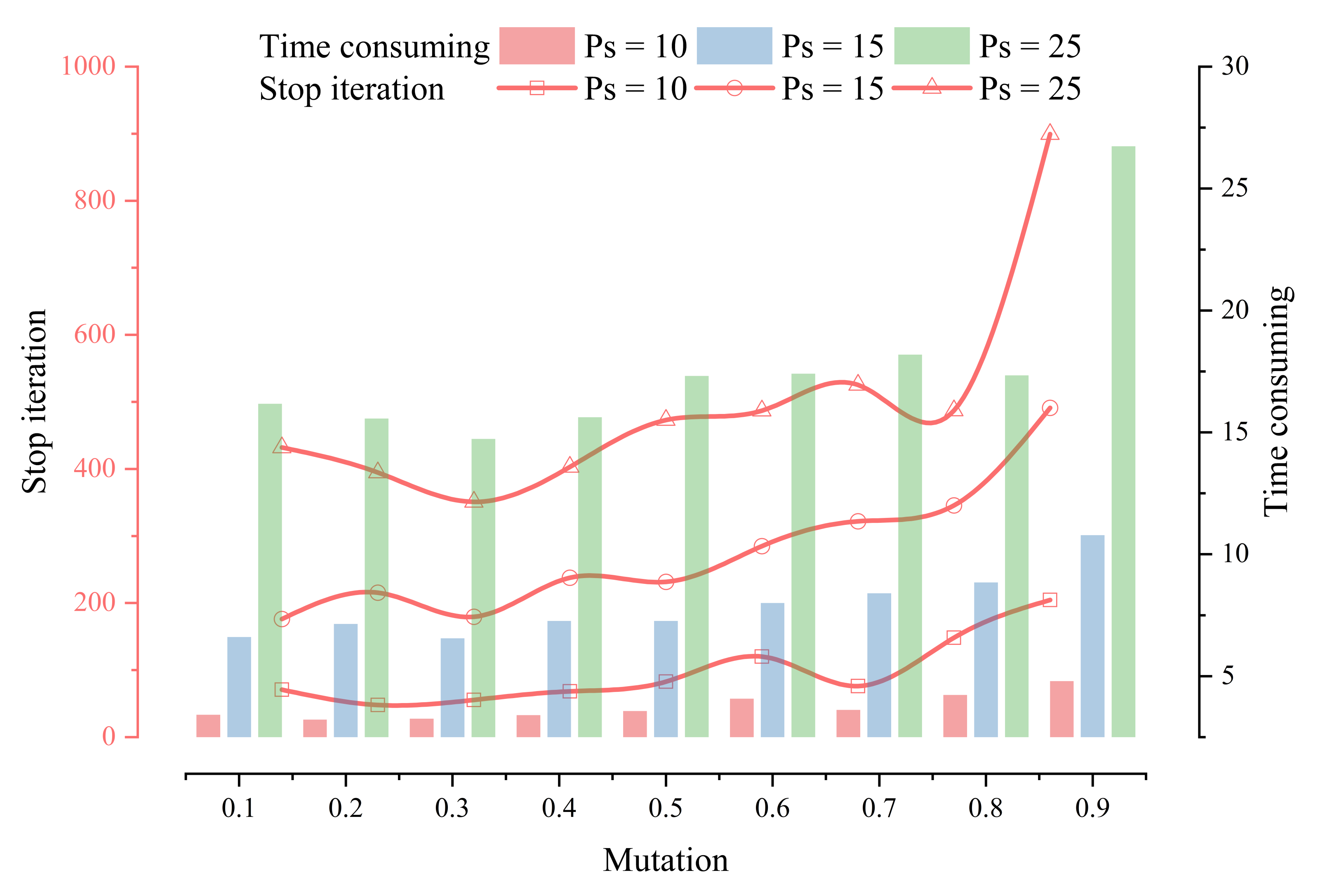
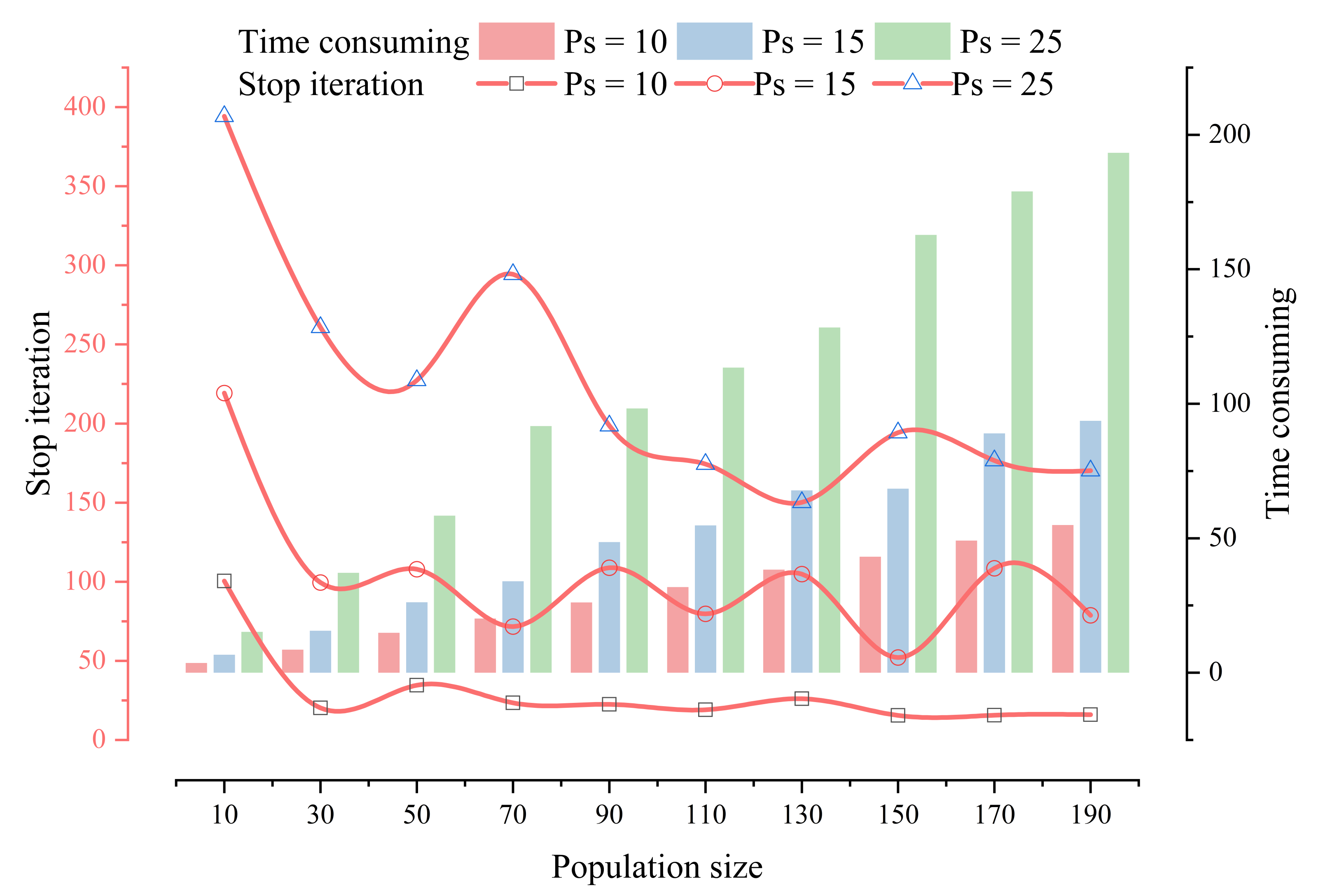
In this section, the parameter on the performance of the designed GA is analyzed, where the mutation value is 0.1 to 0.9, the problem scale is 10 to 25, and the population size is 20 to 200. The specific value and description are shown in

Table 8. Input parameters.

Parameter	Description	Value
$p_m$	Mutation probelity	[0.1, 0.2, 0.3, …, 0.9]
$p_s$	Problem scale	[10, 15, 20, 25]
$Po{p}_s$	Population size	[20, 40, 60, …, 200]
$Stop$	Stop interation	300

, and the analysis results are shown in

Table 9. Mutation parameter sensitivity analysis results.

Mutation	Problem Scale	Population Size	Stop Iteration	Time Consuming (s)
0.1	10	10	70.8	3.4233
0.2	10	10	47.9	3.2185
0.3	10	10	55.4	3.2602
0.4	10	10	68.3	3.4009
0.5	10	10	82.8	3.5706
0.6	10	10	120.2	4.0804
0.7	10	10	76.2	3.6183
0.8	10	10	148.2	4.2285
0.9	10	10	204.7	4.797
0.1	15	10	176.2	6.6113
0.2	15	10	215.5	7.1453
0.3	15	10	179.6	6.556
0.4	15	10	237.8	7.2671
0.5	15	10	231.7	7.2691
0.6	15	10	284.9	8.0006
0.7	15	10	321.9	8.4016
0.8	15	10	345.7	8.8456
0.9	15	10	491	10.7841
0.1	25	10	431.9	16.176
0.2	25	10	394.7	15.5663
0.3	25	10	351	14.7319
0.4	25	10	402.9	15.6192
0.5	25	10	473	17.3146
0.6	25	10	487	17.4071
0.7	25	10	525.4	18.1925
0.8	25	10	487.1	17.3405
0.9	25	10	899.5	26.7369

and

Table 10. Population size sensitivity analysis results.

Population Size	Problem Scale	Mutation	Stop Iteration	Time Consuming (s)
10	10	0.3	100.4	3.606
30	10	0.3	20.2	8.591
50	10	0.3	34.6	14.887
70	10	0.3	23.4	20.126
90	10	0.3	22.5	26.162
110	10	0.3	19.1	31.853
130	10	0.3	26.1	38.343
150	10	0.3	15.5	43.158
170	10	0.3	15.6	49.136
190	10	0.3	16	54.902
10	15	0.3	219.3	6.712
30	15	0.3	99.5	15.649
50	15	0.3	107.9	26.186
70	15	0.3	71.7	33.988
90	15	0.3	108.8	48.568
110	15	0.3	79.7	54.774
130	15	0.3	104.8	67.844
150	15	0.3	52.1	68.42
170	15	0.3	108.5	88.994
190	15	0.3	78.8	93.672
10	25	0.3	394.2	15.205
30	25	0.3	260.8	37.12
50	25	0.3	227.3	58.373
70	25	0.3	294.3	91.735
90	25	0.3	198.7	98.265
110	25	0.3	174.4	113.482
130	25	0.3	150.2	128.371
150	25	0.3	194.3	162.77
170	25	0.3	176.6	178.959
190	25	0.3	170.2	193.299

, which indicates that the performance of GA along with generations in terms of objective function value and computational time for a small-, medium-, and large-sized case, respectively. Figure 8 shows that as the problem scale or the population size increases, the time consumption and the number of stop iteration would also increase, where the population size is a fixed value of 20. Moreover, when the mutation value is 0.9, the time consumption is larger than other mutation values. According to the analysis, when the mutation value is 0.3, the time consumption is the lowest. Figure 9 shows the same scenarios as Figure 8 in terms of the relationship between problem scale and time consumption, where the mutation value is 0.3. Moreover, the larger the population size, the smaller the number of stop iterations. Therefore, in practical application, the specific value of mutation and population size should be designed based on the problem scale.

7. Discussion, Conclusions, and Future Work

In this research, we aimed to improve ship efficiency, reduce ship waiting time, and enhance the adaptability of traditional ship scheduling optimization models to uncertain factors. A traditional ship scheduling model was fuzzified by introducing triangular fuzzy numbers, and a heuristic scheduling algorithm based on the genetic algorithm was established. Taking into account the difference in computational efficiency between online and offline calculations, an algorithm based on tide height and UKC to determine a feasible tidal time window was proposed. The contribution of this research can be divided into the following points:

• By introducing the concept of the time window, the nonlinear tidal height constraint problem is transformed into a linearization problem, and an algorithm for calculating the navigable tide time window of a ship is proposed;
• The fuzzy ship scheduling method based on fuzzy theory provides an effective solution to the ship scheduling optimization problem under uncertain conditions and has higher optimization accuracy than general priority scheduling methods;
• The parameter sensitivity of the optimization solution method designed based on the genetic algorithm is analyzed experimentally, which provides a reference for the application of the model and improves the practicality of the model.

In summary, fuzzy theory was successfully applied to ship scheduling optimization in this study, and an optimization method based on the GA that can improve scheduling efficiency was also designed. The established model and optimization method not only improve the efficiency of ship traffic but also improve the adaptability of the dispatch model to uncertain factors. In the future, this method can be applied to the one-way ship scheduling problem; however, considering that the precise time point is required in real-time scheduling, the correlation between dynamic scheduling and uncertain scheduling needs to be studied in the future.

References

- Akbulaev, N.; Bayramli, G. Maritime transport and economic growth: Interconnection and influence (an example of the countriesin the Caspian sea coast; Russia, Azerbaijan, Turkmenistan, Kazakhstan and Iran). Mar. Policy 2020, 118, 104005. [Google Scholar] [CrossRef]
- Dui, H.; Zheng, X.; Wu, S. Resilience analysis of maritime transportation systems based on importance measures. Reliab. Eng. Syst. Saf. 2021, 209, 107461. [Google Scholar] [CrossRef]
- Bagoulla, C.; Guillotreau, P. Maritime transport in the French economy and its impact on air pollution: An input-output analysis. Mar. Policy 2020, 116, 103818. [Google Scholar] [CrossRef]
- Dulebenets, M. The vessel scheduling problem in a liner shipping route with heterogeneous fleet. Int. J. Civ. Eng. 2018, 16, 19–32. [Google Scholar] [CrossRef]
- Sakawa, M.; Mori, T. An efficient genetic algorithm for job-shop scheduling problems with fuzzy processing time and fuzzy duedate. Comput. Ind. Eng. 1999, 36, 325–341. [Google Scholar] [CrossRef]
- Davis, L. Job shop scheduling with genetic algorithms. In Proceedings of the an International Conference on Genetic Algorithms and Their Applications, Pittsburgh, PA, USA, 24–26 July 1985; Volume 140. [Google Scholar]
- Tanaka, K. Single machine scheduling with fuzzy due dates. In Proceedings of the VII International Fuzzy Systems Association World Congress, IFSA’97, Prague, Czech Republic, 25–29 June 1997; pp. 30–35. [Google Scholar]
- Zhang, X.; Lin, J.; Guo, Z.; Liu, T. Vessel transportation scheduling optimization based on channel–berth coordination. Ocean Eng. 2016, 112, 145–152. [Google Scholar] [CrossRef]
- Zhang, X.; Chen, X.; Ji, M.; Yao, S. Vessel scheduling model of a one-way port channel. J. Waterw. Port Coast. Ocean Eng. 2017, 143, 04017009. [Google Scholar] [CrossRef]
- Zhang, X.; Li, R.; Chen, X.; Li, J.; Wang, C. Multi-object-based Vessel Traffic Scheduling Optimisation in a Compound Waterway of a Large Harbour. J. Navig. 2019, 72, 609–627. [Google Scholar] [CrossRef]
- Liu, B.; Li, Z.C.; Sheng, D.; Wang, Y. Integrated planning of berth allocation and vessel sequencing in a seaport with one-way navigation channel. Transp. Res. Part B Methodol. 2021, 143, 23–47. [Google Scholar] [CrossRef]
- Jia, S.; Wu, L.; Meng, Q. Joint scheduling of vessel traffic and pilots in seaport waters. Transp. Sci. 2020, 54, 1495–1515. [Google Scholar] [CrossRef]
- Jia, S.; Li, C.L.; Xu, Z. Managing navigation channel traffic and anchorage area utilization of a container port. Transp. Sci. 2019, 53, 728–745. [Google Scholar] [CrossRef]
- Abou Kasm, O.; Diabat, A.; Bierlaire, M. Vessel scheduling with pilotage and tugging considerations. Transp. Res. Part E Logist. Transp. Rev. 2021, 148, 102231. [Google Scholar] [CrossRef]
- Li, J.; Zhang, X.; Yang, B.; Wang, N. Vessel traffic scheduling optimization for restricted channel in ports. Comput. Ind. Eng. 2021, 152, 107014. [Google Scholar] [CrossRef]
- Lalla-Ruiz, E.; Shi, X.; Voß, S. The waterway ship scheduling problem. Transp. Res. Part D Transp. Environ. 2018, 60, 191–209. [Google Scholar] [CrossRef]
- Hill, A.; Lalla-Ruiz, E.; Voß, S.; Goycoolea, M. A multi-mode resource-constrained project scheduling reformulation for the waterway ship scheduling problem. J. Sched. 2019, 22, 173–182. [Google Scholar] [CrossRef]
- Ulusçu, Ö.S.; Altıok, T. Waiting time approximation in single-class queueing systems with multiple types of interruptions: Modeling congestion at waterways entrances. Ann. Oper. Res. 2009, 172, 291–313. [Google Scholar] [CrossRef]
- Ulusçu, Ö.S.; Altiok, T. Waiting time approximation in multi-class queueing systems with multiple types of class-dependent interruptions. Ann. Oper. Res. 2013, 202, 185–195. [Google Scholar] [CrossRef] [Green Version]
- Wang, S.; Zhu, M.; Kaku, I.; Chen, G.; Wang, M. An improved discrete pso for tugboat assignment problem under a hybrid scheduling rule in container terminal. Math. Probl. Eng. 2014, 2014, 714832. [Google Scholar] [CrossRef]
- Xu, Q.; Mao, J.; Jin, Z. Simulated annealing-based ant colony algorithm for tugboat scheduling optimization. Math. Probl. Eng. 2012, 2012, 246978. [Google Scholar] [CrossRef] [Green Version]
- Wei, X.; Jia, S.; Meng, Q.; Tan, K.C. Tugboat scheduling for container ports. Transp. Res. Part E Logist. Transp. Rev. 2020, 142, 102071. [Google Scholar] [CrossRef]
- Kang, L.; Meng, Q.; Tan, K.C. Tugboat scheduling under ship arrival and tugging process time uncertainty. Transp. Res. Part E Logist. Transp. Rev. 2020, 144, 102125. [Google Scholar] [CrossRef]
- Liu, D.; Shi, G.; Hirayama, K. Vessel Scheduling Optimization Model Based on Variable Speed in a Seaport with One-Way Navigation Channel. Sensors 2021, 21, 5478. [Google Scholar] [CrossRef]
- Chen, Z.L.; Lei, L.; Zhong, H. Container vessel scheduling with bi-directional flows. Oper. Res. Lett. 2007, 35, 186–194. [Google Scholar] [CrossRef]
- Zhang, B.; Zheng, Z. Model and algorithm for vessel scheduling optimisation through the compound channel with the consideration of tide height. Int. J. Ship. Trans. Logist. 2021, 13, 445–461. [Google Scholar] [CrossRef]
- Zhang, B.; Zheng, Z. Model and Algorithm for Vessel Scheduling through a One-Way Tidal Channel. J. Waterw. Port Coast. Ocean Eng. 2020, 146, 04019032. [Google Scholar] [CrossRef]
- Kelareva, E.; Brand, S.; Kilby, P.; Thiébaux, S.; Wallace, M. CP and MIP methods for ship scheduling with time-varying draft. In Proceedings of the Twenty-Second International Conference on Automated Planning and Scheduling, São Paulo, Brazil, 19–25 June 2012. [Google Scholar]
- Wu, L.; Jia, S.; Wang, S. Pilotage planning in seaports. Eur. J. Oper. Res. 2020, 287, 90–105. [Google Scholar] [CrossRef]
- Lei, D. Fuzzy job shop scheduling problem with availability constraints. Comput. Ind. Eng. 2010, 58, 610–617. [Google Scholar] [CrossRef]
- Lei, D. A genetic algorithm for flexible job shop scheduling with fuzzy processing time. Int. J. Prod. Res. 2010, 48, 2995–3013. [Google Scholar] [CrossRef]
- Lei, D. Co-evolutionary genetic algorithm for fuzzy flexible job shop scheduling. Appl. Soft Comput. 2012, 12, 2237–2245. [Google Scholar] [CrossRef]
- Abdullah, S.; Abdolrazzagh-Nezhad, M. Fuzzy job-shop scheduling problems: A review. Inf. Sci. 2014, 278, 380–407. [Google Scholar] [CrossRef]
- Demir, Y.; İşleyen, S.K. An effective genetic algorithm for flexible job-shop scheduling with overlapping in operations. Int. J. Prod. Res. 2014, 52, 3905–3921. [Google Scholar] [CrossRef]
- Behnamian, J. Survey on fuzzy shop scheduling. Fuzzy Optim. Decis. Mak. 2016, 15, 331–366. [Google Scholar] [CrossRef]
- Liu, C.; Xiang, X.; Zheng, L. A two-stage robust optimization approach for the berth allocation problem under uncertainty. Flex. Serv. Manuf. J. 2020, 32, 425–452. [Google Scholar] [CrossRef]
- Xiang, X.; Liu, C.; Miao, L. A bi-objective robust model for berth allocation scheduling under uncertainty. Transp. Res. Part E Logist. Transp. Rev. 2017, 106, 294–319. [Google Scholar] [CrossRef]
- Xiang, X.; Liu, C. An expanded robust optimisation approach for the berth allocation problem considering uncertain operation time. Omega 2021, 103, 102444. [Google Scholar] [CrossRef]
- Ishii, H.; Tada, M. Single machine scheduling problem with fuzzy precedence relation. Eur. J. Oper. Res. 1995, 87, 284–288. [Google Scholar] [CrossRef]
- Tsujimura, Y.; Gen, M.; Kubota, E. Solving job-shop scheduling problem with fuzzy processing time using genetic algorithm. J. Jpn. Soc. Fuzzy Theory Syst. 1995, 7, 1073–1083. [Google Scholar] [CrossRef] [Green Version]
- Gen, M.; Ida, K.; Cheng, C. Multirow machine layout problem in fuzzy environment using genetic algorithms. Comput. Ind. Eng. 1995, 29, 519–523. [Google Scholar] [CrossRef]
- Sakawa, M.; Kubota, R. Fuzzy programming for multiobjective job shop scheduling with fuzzy processing time and fuzzy duedate through genetic algorithms. Eur. J. Oper. Res. 2000, 120, 393–407. [Google Scholar] [CrossRef]
- Xu, Y.; Wang, L.; Wang, S.Y.; Liu, M. An effective teaching–learning-based optimization algorithm for the flexible job-shop scheduling problem with fuzzy processing time. Neurocomputing 2015, 148, 260–268. [Google Scholar] [CrossRef]
Figure 1.
Simplified sketches of ship entry and exit operation procedures.
Figure 2.
Simplified distance-time sketch with fuzzy speed.
Figure 3.
Process of determining the feasible tidal time window restricted by the tide height.
Figure 4.
Triangular fuzzy number.
Figure 5.
The framework of optimal scheduling where vessel speeds are uncertain.
Figure 6.
Crossover operation and mutation operation. (a) Crossover operator. (b) mutation operator—reverse. (c) mutation operator—insert. (d) mutation operator—swap.
Figure 7.
Feasible tidal time window for vessels. The horizon lines are vessel time windows, the vertical lines are the period, and the red points are the estimated time of arrival.
Figure 8.
Performance in terms of time consuming and mutation parameter for different problem scale.
Figure 9.
Performance in terms of time consuming and population size for different problem scale.