Wind Features Extracted from Weather Simulations for Wind-Wave Prediction Using High-Resolution Neural Networks

Abstract

Nearshore wave forecasting is susceptible to changes in regional wind fields and environments. However, surface wind field changes are difficult to determine due to the lack of in situ observational data. Therefore, accurate wind and coastal wave forecasts during typhoon periods are necessary. The purpose of this study is to develop artificial intelligence (AI)-based techniques for forecasting wind–wave processes near coastal areas during typhoons. The proposed integrated models employ combined a numerical weather prediction (NWP) model and AI techniques, namely numerical (NUM)-AI-based wind–wave prediction models. This hybrid model comprising VGGNNet and High-Resolution Network (HRNet) was integrated with recurrent-based gated recurrent unit (GRU). Termed mVHR_GRU, this model was constructed using a convolutional layer for extracting features from spatial images with high-to-low resolution and a recurrent GRU model for time series prediction. To investigate the potential of mVHR_GRU for wind–wave prediction, VGGNet, HRNet, and Two-Step Wind-Wave Prediction (TSWP) were selected as benchmark models. The coastal waters in northeast Taiwan were the study area. The length of the forecast horizon was from 1 to 6 h. The mVHR_GRU model outperformed the HR_GRU, VGGNet, and TSWP models according to the error indicators. The coefficient of mVHR_GRU efficiency improved by 13% to 18% and by 13% to 15% at the Longdong and Guishandao buoys, respectively. In addition, in a comparison of the NUM–AI-based model and a numerical model simulating waves nearshore (SWAN), the SWAN model generated greater errors than the NUM–AI-based model. The results of the NUM–AI-based wind–wave prediction model were in favorable accordance with the observed results, indicating the feasibility of the established model in processing spatial data.

1. Introduction

Taiwan is located at the turning point of most typhoon paths in the western North Pacific–East Asia region [1]. Strong winds accompany typhoons, and storm surges, an abnormal rise in sea level, can cause damage to offshore facilities near coastal areas. Taiwan’s high mountains play a pivotal role in changing the wind distribution of typhoons around the island and in reducing wind speeds. When waves abate under weakened winds, they become unpredictable [2]. Therefore, a useful scheme for wind–wave forecasting during typhoons is highly desirable for Taiwan.

Coastal waves are highly correlated to local coastal winds in small basins, such as lakes, or under influence of very extreme events, such as typhoons [3,4]. However, changes in coastal land and offshore wind fields cannot be comprehensively examined because in situ observations (e.g., those made at onshore weather stations and offshore buoys) are location-specific and lacking in data. Instead of using wind data from a single source, a numerical weather prediction (NWP) model can be used to simulate wind speed changes in wind fields [5]. Many NWP models exhibit significant improvements in forecasting accuracy as a result of the development and refinement of physical modeling and computational techniques [6]. NWP models forecast weather by solving hydrodynamic and thermodynamic equations [7]. The Weather Research and Forecasting (WRF) numerical model [8] developed by the National Center for Atmospheric Research–National Oceanographic and Atmospheric Administration (NOAA) is a commonly used, mesoscale community NWP model [9].

Following advancements in artificial intelligence (AI), more deep learning (DL) algorithms are being applied to the field of natural science. In particular, artificial neural networks (ANNs) are suitable for image recognition and spatiotemporal data processing and are therefore highly valued and extensively researched. However, ANNs do not offer insight into wave propagation processes, which can be provided by full-scale numerical models [10]. Convolutional neural networks (CNNs) use a DL algorithm to input images, assign learnable weights and biases to various objects in the image, and differentiate images from one another [11]. A CNN is composed of one or multiple convolutional layers and fully connected layers that process two-dimensional (2D) data and extract spatial features from the images. Since the introduction of AlexNet [12], various CNNs, such as VGGNet [13], GoogLeNet [14], and ResNet [15], have been developed. The High-Resolution Network (HRNet), proposed by [16], has a CNN architecture that can process high-resolution (HR) images, such as those developed for human pose estimation, which are used for a broad range of vision tasks. HRNet can maintain HR representations through the whole process of the network architecture. These networks can also be applied to wind–wave problems.

Herein, we adopted AI-based techniques for forecasting wind–wave processes near coastal areas during typhoons. The proposed integrated models combined a NWP model and data-driven AI techniques, namely numerical (NUM)-AI-based wind–wave prediction models. The contributions of this study are as follows: (1) wind field simulation results are valuable for Taiwan, particularly those for typhoon periods, when coastal areas are under strong winds and waves. Typhoon circulation is affected by terrain, which increases the complexity of wind field processes. The wind field data obtained from mesoscale meteorological models are highly accurate in reflecting the characteristics of wind fields, which can provide reasonable forced conditions for the simulation of typhoon waves [17]. Accordingly, we employed an NWP WRF model to simulate wind fields, integrated the wind field and in situ observational data, and used them as the input data for the AI-based wind–wave prediction models. (2) After establishing the NUM–AI-based model, we used 2D wind fields as the model input. Spatial feature extraction was performed through the convolutional and pooling layers, and the obtained feature map was used for training the model of wind-induced waves. (3) The NUM–AI-based model comprises a hybrid VGGNet and HRNet model integrated with recurrent-based gated recurrent units (GRUs) and was termed the VHR–GRU model. We combined the two algorithms because they had the following characteristics.

• Regarding spatial data processing, the HRNet [16] model is constructed using convolutional layers, which facilitates feature extraction from images with high-to-low resolution. An HRNet model maintains HR representations by connecting convolutions of high-to-low resolution in parallel and by repeatedly conducting multiscale fusion across parallel convolutions.
• A recurrent-based GRU layer was employed to address the time delays in waves and winds. The GRU layer enables memory block units to determine the memory time length and provide the most effective memory length of time series data on the time axis.

2. Related Work

A typhoon with intense and rapidly varying wind fields forms dramatically different offshore waves under spatiotemporal constraints [18,19,20]. Numerical wave models are based on the concept of a wind–wave energy spectrum, which rises and falls in response to changes in the wind field and the wave energy propagated from other regions. The WAM [21] and WAVEWATCH III [22] for the deep ocean and Simulating WAves Nearshore (SWAN; [23]) for nearshore regions are the most commonly used numerical wave models for estimating ocean waves [24]. The third-generation wave model SWAN has been used extensively to model waves in coastal regions with gradual bathymetric variations [25,26,27]. SWAN has also been widely applied to the numerical simulation of typhoon waves [28,29,30]. Generally, physical models are complex in terms of their input requirements and execution time.

Wind forcing is a key determinant of the wave field [31], and wave models rely on the wind features to simulate the wave fields accurately. Data from in situ observations [32,33,34], remote sensing [35,36,37], and numerical modeling [38,39,40,41] have demonstrated the complex spatial distribution of wind and wave fields.

Multiple AI models, such as multilayer perceptrons [42], recurrent neural networks (RNNs; [43,44]), and CNNs [45], have been developed based on various DL algorithms. Notably, RNNs use their internal state (memory) to process input sequences of variable lengths [46]. Long short-term memory (LSTM) and GRU neural networks are RNNs that can learn the temporal dynamics of sequential data and address the vanishing gradient problem [47,48,49]. RNNs, which efficiently use temporal information for the sequential analysis of input data, are also suitable for addressing wind–wave prediction problems. Huang et al. [50] and Cheng et al. [51] have constructed accurate RNN-based wind speed prediction models, and Sadeghifar et al. [52], Demetriou et al. [53], Zhang et al. [54], and Zhou et al. [55] have conducted coastal wave height prediction using RNN-based models. In addition, in our previous study, we developed a Two-Step Wind-wave Prediction (TSWP) typhoon wind–wave prediction model, using deep RNNs to forecast wind speed and wave height during typhoons. However, because in situ observational data were applied, the wind speed data could not describe the spatial wind field features, resulting in the serious underestimation of peak values.

According to [56], CNNs have two main representations. Low-resolution representations are mainly used for image classification, whereas HR representations are essential for vision problems such as semantic segmentation and object detection. The fully convolutional network (FCN; [57]) computes low-resolution representations through the removal of the fully connected layers in a classification network, performing estimation from their coarse segmentation confidence maps. The FCN model is widely used as the backbone of VGGNet [13]. Studies that have employed low-resolution networks, such as [58,59], determined the spatiotemporal correlations of wind speed prediction using a predictive deep CNN. Silva et al. [60] identified rip currents with breaking waves by using a faster R-CNN. HR representations were maintained throughout the process through the use of a network constructed with connecting multiresolution (from high- to low-resolution) parallel convolutions, with repeated information exchange occurring across parallel convolutions [16]. Representative HR models include GoogLeNet [14], ResNet [15], SegNet [61], and U-Net [62]. Some researchers have studied HR networks in relation to wind–wave predictions. For example, Shivam et al. [63] employed ResNet for short-term wind speed prediction, and Choi et al. [64] estimated significant wave heights from ocean images using VGGNet, GoogLeNet, ResNet, and DenseNet.

HRNet [16], a new-generation HR CNN, maintains HR representations through the connection of convolutions of high-to-low resolution in parallel, where multiscale fusion occurs repeatedly across parallel convolutions. HRNet constitutes a novel convolution operation technique suitable for extracting the spatiotemporal features of wind fields and can therefore be further applied to enhance wind–wave prediction. To examine the prediction performance of high- and low-resolution representations, we compared the performance of the HRNet and VGGNet models with that of an established hybrid model integrating VGGNet, HRNet, and a recurrent-based GRU layer, referred to as the VHR–GRU model. In addition, we used the TSWP model [65] as a benchmark to compare the error range between the TSWP, in which only in situ observational data were applied, and the NUM–AI-based model, in which the NWP-based wind field simulation data were incorporated, and further evaluated whether the NUM–AI-based model could effectively increase prediction accuracy. Although we focused on developing the AI-based wind–wave model, we also analyzed the simulation results of the SWAN model to identify inter-model differences.

3. Framework of the NUM–AI-Based Model

In this section, we describe the methodology of the proposed compound numerical outputs and AI-based models for wind–wave prediction during typhoons. The methodology comprised the following three stages: (1) WRF wind numerical model simulation, (2) NUM–AI-based wind–wave prediction model development, and (3) model verification using numerical SWAN wave model simulations. The methodology diagram in Figure 1 outlines the data flow of these three stages (presented as cloud blocks). The processes of the stage simulations and techniques are described as follows.

3.1. Wind Field Simulation Using the WRF Numerical Model

Advanced Research WRF version 3.9.1 was used to simulate the HR field data of typhoons. WRF is a next-generation mesoscale numerical weather prediction system designed for both atmospheric research and operational forecasting applications. Additional details can be found in the WRF Version 3 Modeling System User’s Guide [66]. The WRF model was employed as the numerical simulation-based model for precomputing numerical solutions to determine the wind field using the grid system. These simulated wind field outcomes are used for training the NUM–AI-based prediction model in the next stage. In this stage, the NOAA National Center for Environmental Prediction (NCEP) Global Data Assimilation System (GDAS) FNL (Final) Operational Global Analysis data were collected for the initial field and boundary conditions. FNL refers to the final analysis and the products from the data assimilation and NCEP global NWP system.

The WRF model provides various options for physical parameters, such as weather patterns, geographic locations, and simulation scenarios. We referred to [17,67,68,69] in selecting the physical parameters. These researchers studied the typhoon track, rainfall, and wind forecasts for WRF model simulations using reasonable physical parameters for typhoons approaching Taiwan. The suitable schemes in the respective WRF typhoon models were as follows: Single-Moment 6-Class Microphysics Scheme [70] for microphysical processes, Yonsei University [71] for the planetary boundary layer, Kain–Fritsch [72] for cumulus convection, Rapid Radiative Transfer Model [73] for long-wave radiation, and Dudhia [74] for short-wave parameters.

3.2. Wave Outcomes Obtained Using the NUM–AI-Based Prediction Model

In this stage, the outcomes of the wind field from the WRF model were used for training the NUM–AI model. The NUM–AI-based prediction model was then developed to predict the wave heights in the study area. Note that the developed NUM–AI model is useful only for specific locations and not for wave field predictions. To train an NUM–AI-based model, the wind field outcomes of the WRF model and in situ data were applied as input attributes, with the wave heights at (t + i)_{i = 1,6} of a buoy representing the target. The forecast horizon was from 1 to 6 h.

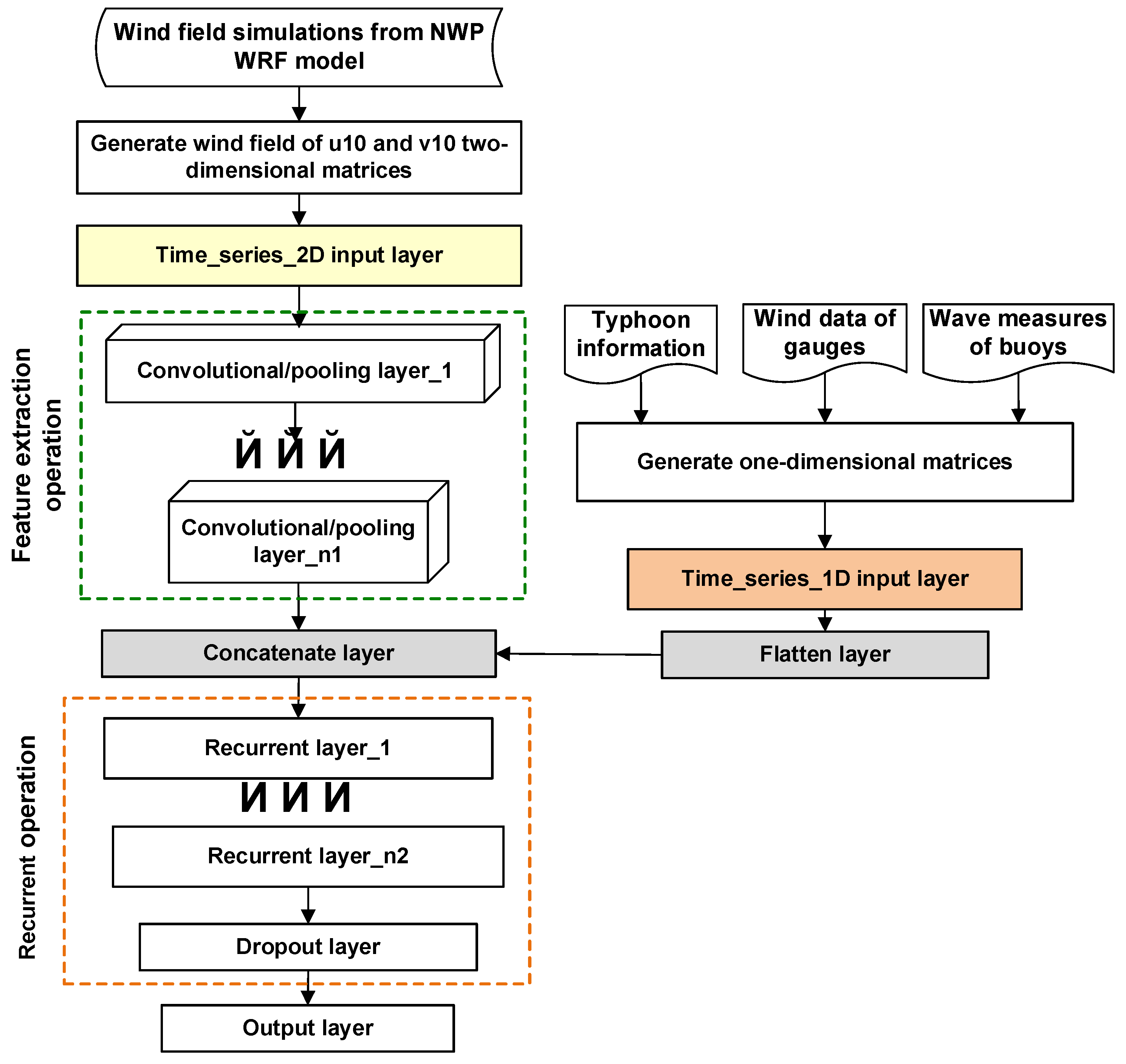
The NUM–AI-based model combines the WRF numerical model with DL techniques to predict winds and waves in the study area. The network of the NUM–AI-based model (Figure 2) executes feature extraction and recurrent operations. First, the feature extraction operation, involving cascade pooling and convolutional layers, was employed to extract the feature maps from the 2D wind field simulated using the WRF model. The recurrent operation was then used to construct the time series-based models. The time series data encompassed the wind field simulated using the WRF model and the in situ observational data (i.e., typhoon information, wind data from gauges, and wave data from buoys) and were transformed into one-dimensional (1D) array data.

As detailed in Figure 2, feature extraction was performed using fully convolutional feature extractors, namely VGGNet [13] and HRNet [16]. We also developed a VGGNNet–HRNet hybrid called VHRNet, which was inspired by the backbones of both architectures. These architectures are described as follows. VGGNet networks [13], such as VGG11 and VGG16 (the common variant of VGGNet; [75]), structurally consists of five blocks of multiple convolutional layers and a single max pooling layer. Herein, the four blocks were employed to ensure consistency with the four-block architecture of HRNet. Figure 3 illustrates the modified VGGNets of VGG11 and VGG16 (termed mV11 and mV16, respectively). The four-block structure of VGG11 uses one, one, two, and two convolutional layers, whereas that of VGG16 uses two, two, three, and three convolutional layers. Both modified VGGNet models completed operations with three fully connected layers.

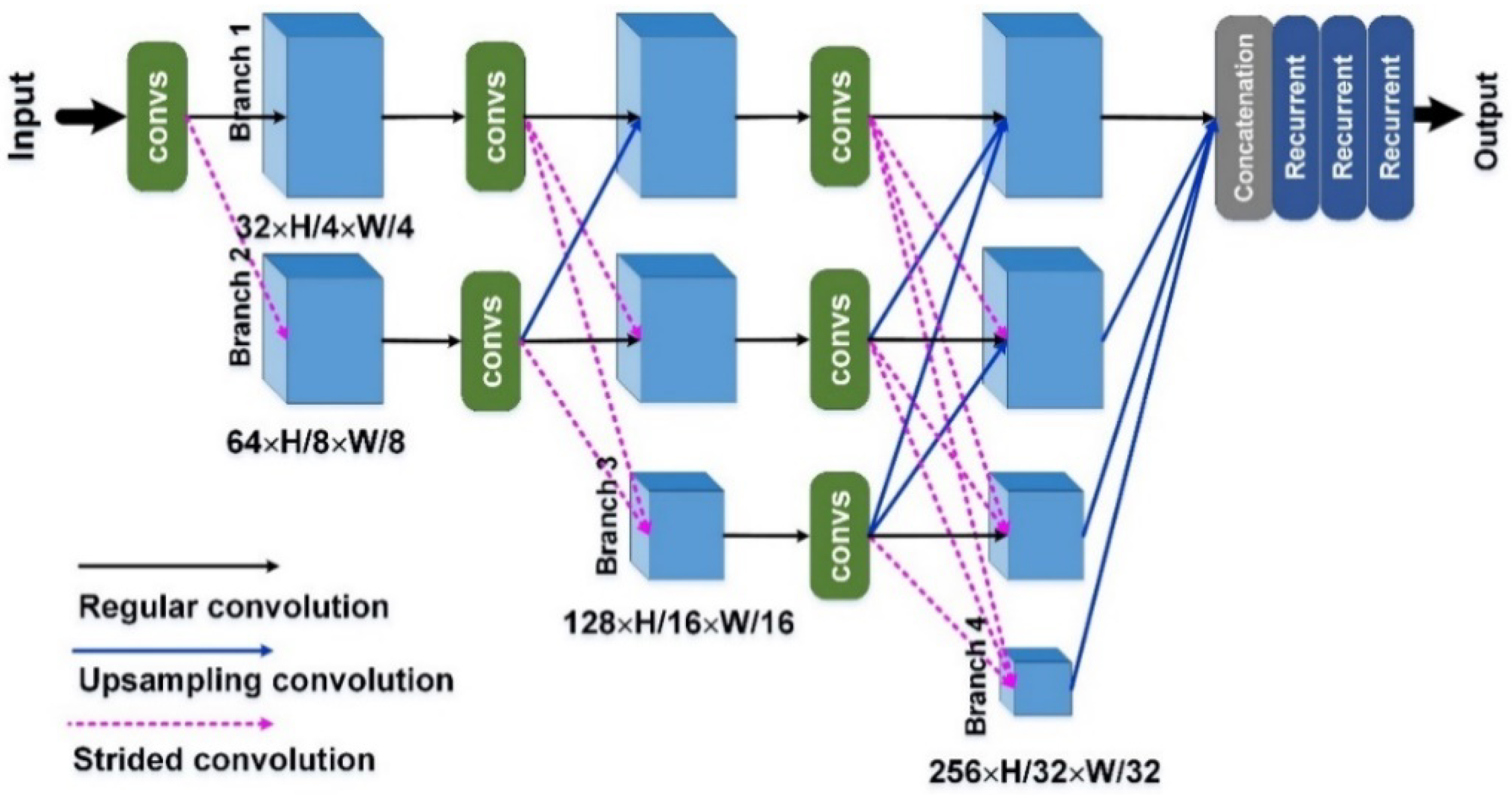
HRNet [16] introduces a multiscale parallel design to produce HR features without requiring a decoding stage. As illustrated in Figure 4, the HRNet architecture consists of four parallel branches [76], with the upper branch (branch 1) storing the spatial details through the convolutions while maintaining HR. In the lower branches (branches 2–4), strided convolutions were applied to reduce the spatial size of the feature maps and enlarge the receptive fields [76]; these branches corresponded to the four high-to-low spatial resolutions. In Figure 4, “convs” refers to a convolutional block consisting of a convolutional layer and a pooling layer.

The proposed mVHRNet is a combination of the modified VGGNet and HRNet architectures (Figure 5). To extract the feature maps, several blocks in the mV11 and mV16 were embedded into the backbone of a HRNet structure (hereafter mV11HR and mV16HR, respectively). In the original HRNet, the first convs block downsamples the inputs to a quarter of their original size. To obtain more spatial information from the input images, we applied half-image downsampling in block 1 of mVHRNet. Furthermore, we added a fifth branch of feature maps at high to low resolution. After feature extraction, the highly abstract features were obtained and fed in a concatenation layer in which 1D and 2D data were fused and flattened into a 1D vector, which was then connected with the fully connected layers. Subsequently, model training with the fully connected layers was performed.

RNNs, although suitable for time series data, are difficult to train and are detrimentally affected by vanishing or exploding gradients; therefore, they cannot solve the long-term dependency problem [77]. Proposed by [49], the GRU is a variant of LSTM, with a gated mechanism in the RNN structure. Specifically, the GRU has two gates (update and reset gates), and the LSTM has three (input, output, and forget gates) [78]. Because the GRU has fewer training parameters and usually converges quicker than the LSTM during training [7], we employed a GRU neural network to compute the temporal dynamics of time series data and shorten the computational time. After the dropout layer, wherein the weights of a certain proportion of nodes are randomly dropped to prevent overfitting, the results are produced from the output layer.

3.3. Comparison with the Wave Numerical Simulations

The SWAN numerical models were used to simulate the nearshore wave field during typhoons to enable comparison with the AI-based model. Additional details can be found in the SWAN User Manual [79]. According to [80,81], the application of the SWAN model to medium- and small-grid networks is suitable for simulating the wave state in nearshore Taiwan. Based on a Eulerian formulation of the discrete spectral balance of action density that accounts for refractive propagation over arbitrary bathymetry and current fields [25], SWAN is driven by boundary conditions and local winds. Here, the wind fields obtained from WRF results were used as inputs for the SWAN model simulations in the study.

To simulate the typhoon waves, the computational domain ranges from 10° to 35° N and 110° to 140° E. The near-field nested computation domains in northern Taiwan at Longdong and Guishandao buoys. The various settings of parameters were referred to [82]. For the far-field wave simulations the grid spacing is 12 km and the 20 exponentially spaced frequencies from 0.01 to 0.5 Hz with 60 evenly spaced directions for a time step of 15 min are used. For numerical computations, a grid size of 2 km and time step of 10 min are used in the coastal nested domain, while in near-field nested domains, a grid size of 300 m and a time step of 5 min are employed. The SWAN simulation results were verified using the wave heights at the experimental sites (Longdong and Guishandao buoys) and were compared against the results obtained from the previous stage of the NUM–AI-based wind–wave prediction model (see Section 5.3).

4. Study Area and Modeling

Figure 6 depicts the experimental area (right part). The left part of the figure indicates the topography of the surroundings of Taiwan [83]. The two buoys at Longdong (water depth of 34 m) and Guishandao (27 m), near Taiwan’s northeastern coast, were the experimental sites. We investigated typhoon events between 2005 and 2019 (

Table 1. Typhoon data from 2005 to 2019.

Year	Typhoon Name and Date	Year	Typhoon Name and Date
2005	Haitang (7/16–7/20), Matsa (8/3–8/6), Longwang (10/1–10/3)	2012	Talim (6/19–6/21), Saola (7/31–8/3), Haikui (8/6–8/7), Tembin (8/21–8/28), Jelawat (9/27–9/28)
2006	Bilis (7/12–7/15), Kaemi (7/23–7/26), Saomai (8/7–8/10), Shanshan (9/14–9/16)	2013	Soulik (7/11–7/13), Trami (8/20–8/22), Kong-rey (8/27–8/29), Usagi (9/20–9/22), Fitow (10/5–10/7)
2007	Wutip (8/8–9), Sepat (8/16–8/19)	2014	Matmo (7/21–7/23), Fung-wong (9/19–9/22)
2008	Kalmaegi (7/16–7/18), Fung-wong (7/26–7/29), Sinlaku (9/11–9/16), Jangmi (9/26–9/29)	2015	Chan-hom (7/9–7/11), Soudelor (8/6–8/8)
2009	Morakot (8/5–8/8)	2016	Malakas (9/16–9/18), Megi (9/26–9/28)
2010	Fanapi (9/18–9/20), Megi (10/21–10/23)	2017	Nesat (7/28–7/30)
2011	Meari (6/23–6/25), Muifa (8/4–8/6), Nanmadol (8/27–8/30)	2019	Lekima (8/7–8/10), Mita (9/29–10/1)

) that affected ocean waves in the northeast offshore area of Taiwan.

The typhoon characteristics, ground-based wind speed data, and buoy wave height data obtained from Taiwan’s Central Weather Bureau (CWB) were collected. The ground-based wind speed data were sourced from four ground stations in Keelung, Yilan, Suao, and Pengjiayu. Information on typhoon characteristics, including the hourly climatologic data, was collected with reference to the pressure at the typhoon center, the maximum radius of winds over 15.5 m/s, the movement speed of the typhoon, and the maximum wind speed at the typhoon center. Surface wind speeds on the ground and notable wave heights at the buoys were sourced from CWB-managed stations.

Table 2. Range and average values of the collected attributes.

Attribute	Unit	Range	Mean
Pressure at typhoon center	hPa	910–998	959
Maximum radius of winds over 15.5 m/s	km	50–300	212
Movement speed of typhoon	km/h	5–43	16.4
Maximum wind speed at typhoon center	m/s	18.1–55.0	36.9
Surface wind speed at Pengjiayu	m/s	0.3–44.3	12.3
Surface wind speed at Keelung	m/s	0–24.0	5.7
Surface wind speed at Yilan	m/s	0–33.4	5.0
Surface wind speed at Suao	m/s	0.1–25.2	4.3
Significant wave height at Longdong	m	0.2–17.1	2.5
Significant wave height at Guishandao	m	0.2–12.6	2.3

lists these attributes by using the minimum, maximum, and mean values of the typhoon, ground, and buoy station information.

4.1. WRF Simulations

We collected the FNL Operational Global Analysis data from the NOAA NCEP GDAS to examine the WRF model’s initial field and boundary conditions. The typhoon information, including the estimated track, intensity, and strength of the typhoons, was collected from the Regional Specialized Meteorological Center Tokyo–Typhoon Center of the Japan Meteorological Agency. A two-level nested grid was set (Figure 7).

The outer domain (Domain 1) included the typhoon movement path ranging between 117° E–132° E and 15° N–30° N, with a 15-km resolution (grid size = 0.15°, number of grids = 100 × 100). The inner domain (Domain 2) included the simulated circulation systems of medium- and small-scale typhoons and the wind- and wave-forming areas in northeastern Taiwan. To more precisely describe the spatial scale and resolution of wind-generating waves in Domain 2, we referred to [81], setting the range between 120° E–125.12° E and 22° N–27.12° N, with a 4-km resolution (grid size = 0.04°, number of grids = 128 × 128). Furthermore, 32 vertical levels were set. Each typhoon was simulated for several consecutive days, with numerical prediction and analysis conducted four times a day for 12 h each time.

4.2. Model Construction

We used the WRF model to simulate the hourly wind fields of the 38 typhoons in the study area listed in Table 1. After the simulations, the wind field analysis data, such as the x- and y-plane axes and the z height axis of each typhoon event, were obtained. The output data of the WRF model constituted the surface wind field data (including u10 and v10, the x- and y-axis wind speed, respectively) and were used as the input data for the coastal wind–wave simulations [81]. Therefore, we output the wind field data at a surface height of 10 m, obtaining the simulation values of 2436 pieces of hourly data. To establish the NUM–AI-based model, data partitioning was conducted according to the sequence of the typhoons. The training set was composed of the data of 24 typhoons from 2005 to 2012 (accounting for 63% of the total number of typhoons, with 1562 pieces of hourly data). The validation set comprised the five 2013 typhoons (accounting for 13% of the total typhoons, with 270 pieces of hourly data), and the testing set consisted of nine typhoons occurring between 2014 and 2019 (accounting for 24% of the total typhoons, with 604 pieces of hourly data).

We employed the Python programming language to establish the models, with the Tensorflow (version 2.3) and Keras libraries of Python used for model computation. When constructing an NUM_AI-based model, feature extraction processing is first initiated, and the 2D matrices of the wind fields are passed through the four-block architectures of mV16, HRNet, and mVHRNet (Figure 3, Figure 4 and Figure 5). The 2D matrices of 128 × 128 pixels generated by the WRF model (using Domain 2) served as the inputs for the model calculations. These 2D wind field inputs were then encoded into two channels, u10 and v10. The settings of the three convolutional feature extractors are described as follows. For the modified VGGNet, the parameter settings were as follows. The kernel size was 3, the padding method was “same”, the max pooling involved a pool size of 2, and the activation function was the rectified linear unit (ReLU). The number of filters in blocks 1–5 was 32, 64, 128, and 256, respectively.

For HRNet, the parameter settings were as follows. The kernel size is 3 in each convs, the padding method was “same”, the max pooling involved a pool size of 4, and the activation function was ReLU. The stride size of the strided convolution was 2. The resolution increase was implemented through the bilinear upsampling approach [56]. The number of filters in the four convs was 32, 64, 128, and 256, respectively.

For mVHRNet, the parameter settings were as follows. The kernel size was 3 in blocks 1 to 4, the padding method was “same”, the max pooling involved a pool size of 2, and the activation function was ReLU. The stride size of the strided convolution was 2, and the upsampling approach was the same as that employed in HRNet. The number of filters in blocks 1–4 was 32, 64, 128, and 256, respectively.

After the 2D feature maps and 1D attributes were flattened, both flattened arrays were combined using a concatenate layer. Next, the GRU layers were applied under the following settings. The activation function was ReLU, the dropout rate of the dropout layer was 0.2, min–max normalization was used to rescale the range of features in (0, 1), the loss function was the mean squared errors, the metric was the root-mean-square errors (RMSEs), the epoch size was 300, and the optimizer was an adaptive moment estimation optimizer with the standard parameter values (l = 10⁻³, b₁ = 0.9, b₂ = 0.999, e = 10⁻⁸) recommended by [84]. This provided sufficient training time for even the slowest-learning architectures to reach a validation plateau.

The hyperparameters of the number of GRU layers and the number of neurons in a GRU layer were calibrated; their calibration ranges were 1 to 5 and 200 to 2000, respectively. The parameter calibrations of five models, mV11_GRU, mV16_GRU, HR_GRU, mV11HR_GRU, and mV16HR_GRU, with feature extractors connecting to GRU, are listed in

Table 3. Parameter calibrations for the number of GRU layers and number of neurons in a GRU layer at the Longdong buoy.

Parameters	Number of Layers and Neurons with Their Corresponding RMSE (m)
Lead time (h)	t + 1	t + 2	t + 3	t + 4	t + 5	t + 6
mV11_GRU	1, 780 (0.582)	1, 800 (0.852)	2, 560 (1.001)	2, 540 (1.230)	2, 720 (1.367)	2, 720 (1.459)
mV16_GRU	2, 540 (0.571)	2, 560 (0.845)	2, 680 (0.962)	2, 860 (1.119)	3, 940 (1.356)	2, 1340 (1.451)
HR_GRU	2, 780 (0.549)	2, 740 (0.829)	2, 840 (0.946)	3, 840 (1.079)	2, 1340 (1.248)	3, 1140 (1.375)
mV11HR_GRU	3, 920 (0.542)	2, 880 (0.817)	3, 840 (0.941)	2, 1240 (1.078)	3, 1080 (1.228)	4, 980 (1.359)
mV16HR_GRU	2, 1040 (0.483)	3, 960 (0.810)	3, 1120 (0.933)	3, 1000 (1.046)	3, 1320 (1.215)	4, 920 (1.350)

and

Table 4. Parameter calibration for the number of GRU layers and number of neurons in a GRU layer at the Guishandao buoy.

Parameters	Number of Layers and Neurons with Their Corresponding RMSE (m)
Lead time (h)	t + 1	t + 2	t + 3	t + 4	t + 5	t + 6
mV11_GRU	1, 660 (0.514)	1, 680 (0.652)	1, 920 (0.786)	2, 520 (0.879)	2, 920 (0.963)	2, 880 (1.224)
mV16_GRU	1, 980 (0.498)	1, 1080 (0.644)	2, 760 (0.785)	2, 840 (0.877)	2, 900 (0.961)	2, 1140 (1.228)
HR_GRU	1, 1020 (0.472)	2, 820 (0.617)	2, 860 (0.757)	3, 840 (0.868)	2, 1200 (0.946)	3, 960 (1.128)
mV11HR_GRU	2, 780 (0.466)	2, 940 (0.613)	2, 1080 (0.749)	3, 1120 (0.853)	2, 1100 (0.932)	3, 980 (1.024)
mV16HR_GRU	2, 960 (0.458)	2, 860 (0.618)	2, 1040 (0.750)	3, 1340 (0.854)	3, 1220 (0.936)	3, 1040 (1.024)

. The calibration results of the optimal parameters obtained using a validation set from the Longdong and Guishandao buoys are displayed. Possible parameter combinations were searched, and those with the smallest RMSEs were retained as the optimal parameters. The RMSE is defined as

$$\mathrm{RMSE}=\sqrt{\frac{1}{\mathrm{N}}{{\displaystyle \sum }}_{i=1}^{\mathrm{N}}{\left(P_i-O_i\right)}^2},$$

(1)

where N is the total number of observations, $P_i$ is the predicted wave height at record i, and $O_i$ is the observed wave height at record i.

5. Results and Discussion

5.1. Typhoon Testing and Prediction

We used multiple typhoons in the testing set for model prediction and evaluation. Figure 8 and Figure 9 illustrate the predicted wave height values within a lead time of 1 to 6 h from the Longdong and Guishandao buoys in relation to the typhoon test set. The optimal parameters obtained in Section 4 (i.e., mV11_GRU, mV16_GRU, HR_GRU, mV11HR_GRU, and mV16HR_GRU) were applied for prediction. Furthermore, the TSWP model was employed to compare the differences in performance of models employing observation data only versus employing both observation data and NWP wind simulation data. In these figures, we found that prediction accuracy was inversely related to the lead time. This is because when the prediction time length was longer, the uncertainty of the wind–wave readings increased. However, the waveform changes were still discernible overall. Moreover, when the lead time reached 4 h and above, the prediction values tended to underestimate peak values and add a delay. A possible cause is that the rapidly changing typhoon circulation structure leading to the WRF weather simulation increasing the higher wind errors when future time t > = 4 h.

5.2. Model Performance Levels

To examine the prediction errors of each model, evaluation indicators, namely the RMSE, relative RMSE (rRMSE), mean absolute error (MAE), and relative mean absolute error (rMAE), were measured. These are defined as follows:

$$\mathrm{rRMSE}=\frac{\mathrm{RMSE}}{\overline{O}}$$

(2)

$$\mathrm{MAE}=\frac{1}{\mathrm{N}}{{\displaystyle \sum }}_{i=1}^{\mathrm{N}}\left|P_i-O_i\right|$$

(3)

$$\mathrm{rMAE}=\frac{\mathrm{MAE}}{\overline{O}}$$

(4)

where $\overline{O}$ is the average of all the observed wave heights at a specific buoy. The MAE measures the average magnitude of the errors in a set of forecasts, indicating that all the individual differences are weighted equally in the average calculation. The RMSEs are squared before they are averaged, conferring a relatively high weight to large errors; thus, this measure is most useful when large errors are particularly undesirable [85].

Figure 10 presents the RMSEs, rRMSEs, MAEs, and rMAEs of the data from both buoys. The performance of HR_GRU, mV11HR_GRU, and mV16HR_GRU was more satisfactory than those of mV11_GRU, mV16_GRU, and the TSWP model. In sum, the three HR-based structures exhibited relatively few prediction errors at high values and less bias compared with the actual observation values.

Table 5. Averages of the RMSE and MAE and their IR for a lead time of 1 to 6 h at the Longdong and Guishandao buoys.

Buoy	Model	RMSE (m)	rRMSE	MAE (m)	rMAE	IRRMSE	IRMAE
Longdong	mV11_GRU	1.136	0.445	0.692	0.271	6.44%	4.06%
	mV16_GRU	1.116	0.437	0.687	0.269	8.06%	4.81%
	HR_GRU	1.085	0.425	0.634	0.248	10.64%	12.15%
	mV11HR_GRU	1.049	0.411	0.595	0.233	13.61%	17.45%
	mV16HR_GRU	1.036	0.405	0.585	0.229	14.71%	18.95%
	TSWP	1.214	0.475	0.721	0.282	-	-
Guishandao	mV11_GRU	1.031	0.424	0.637	0.262	5.62%	7.43%
	mV16_GRU	1.022	0.420	0.642	0.264	6.49%	6.82%
	HR_GRU	0.983	0.405	0.590	0.242	10.06%	14.37%
	mV11HR_GRU	0.972	0.400	0.570	0.234	11.03%	17.29%
	mV16HR_GRU	0.975	0.401	0.589	0.242	10.78%	14.42%
	TSWP	1.093	0.449	0.689	0.283	-	-

presents a summary of the mean RMSE and MAE over a lead time of 1 to 6 h. Compared with the observation values from the Longdong buoy, the mean RMSE and MAR of mV16HR_GRU were the most satisfactory among the remaining models, as were the mean RMSE and MAE of mV11HR_GRU for the observed values at the Guishandao buoy. On the basis of the error indicators of the TSWP model, we defined the improvement rate (IR) for the RMSE and MAE of the models as follows:

$$\mathrm{IR}=\left(X_{\mathrm{TSWP}}-X_k\right)/X_{\mathrm{TSWP}},$$

(5)

where X_k is the metric (i.e., RMSE and MAE) of a specific model k and X_TSWP is the metric of the TSWP model.

The results of the calculation (Table 5) are as follows. (1) With regard to the observation values from the Longdong buoy, the RMSE of the three HR-based models improved by 10% to 15% compared to the TSWP model, whereas the MAE improved by 12% to 19%. The RMSE and MAE of the mV11_GRU and mV16_GRU models improved by 6% to 9% and by 4% to 5%, respectively. (2) In terms of the observation data from the Guishandao buoy, the IR in the RMSE (IR_RMSE) of the three HR-based structures was 10% to 12%, and the IR in the MAE (IR_MAE) was 14% to 18%. The IR_RMSE and IR_MAE of the mV11_GRU and mV16_GRU models were 5% to 7% and 6% to 8%, respectively. Compared with the VGG-based models, the HR-based models more effectively reduced the error between the observed and predicted values. This may be attributable to the HR-based models’ integration of feature maps with high-to-low resolution; the VGG-based models only integrated images with a single spatial resolution. Therefore, the HR-based models generated superior calculation results.

In addition, the efficiency coefficient CE, which indicates the goodness-of-fit, was used, as was the correlation coefficient r. They are defined as

$$\mathrm{CE}=1-\frac{{{\displaystyle \sum }}_{i=1}^{\mathrm{N}}{(P_i-O_i)}^2}{{{\displaystyle \sum }}_{i=1}^{\mathrm{N}}{(O_i-\overline{O})}^2},$$

(6)

$$\mathrm{r}=\frac{{{\displaystyle \sum }}_{i=1}^{\mathrm{N}}\left(P_i-\overline{P}\right)\left(O_i-\overline{O}\right)}{\sqrt{{{\displaystyle \sum }}_{i=1}^{\mathrm{N}}{\left(P_i-\overline{P}\right)}^2{{\displaystyle \sum }}_{i=1}^{\mathrm{N}}{\left(O_i-\overline{O}\right)}^2}}$$

(7)

where $\overline{P}$ is the average of all the predicted wave heights at a specific buoy.

Figure 11 plots the CE and r of the data from both buoys. Figure 11a,b illustrates the reduction in the CE and r along with the increase in the forecast horizon. The three HR-based models had higher prediction efficiency. The increasing forecast horizon verified that the HR-based models maintained higher prediction efficiency than did the VGG-based models and TSWP model. The CE of the HR-based models was not substantially reduced.

Table 6. Averages of CE and r and their IR at the lead time of 1 to 6 h at the Longdong and Guishandao buoys.

Buoy	Model	CE	r	IRCE	IRr
Longdong	mV11_GRU	0.676	0.826	8.43%	1.49%
	mV16_GRU	0.688	0.836	10.32%	2.80%
	HR_GRU	0.705	0.845	13.04%	3.90%
	mV11HR_GRU	0.725	0.850	16.27%	4.47%
	mV16HR_GRU	0.731	0.856	17.30%	5.17%
	TSWP	0.624	0.814	-	-
Guishandao	mV11_GRU	0.629	0.791	7.70%	2.52%
	mV16_GRU	0.635	0.799	8.75%	3.47%
	HR_GRU	0.662	0.815	13.37%	5.59%
	mV11HR_GRU	0.671	0.820	14.86%	6.26%
	mV16HR_GRU	0.669	0.817	14.49%	5.85%
	TSWP	0.584	0.772	-	-

lists the mean CE and r and the evaluation data for improvement efficiency. The analytical results indicated that mV16HR_GRU and mV11HR_GRU had the highest CE and r compared with the observation data from the Longdong and Guishandao buoys. The prediction efficiency of the HR-based models (HR_GRU, mV11HR_GRU, and mV16HR_GRU) differed according to the testing site. mV16HR_GRU requires more layers of convolution operations than does mV11HR_GRU; therefore, a more complex network structure was required for prediction at the Longdong buoy to generalize problems and effectively represent the testing site. In terms of the marine environment, the Longdong buoy is closer to the coast (approximately 1 km away) than the Guishandao buoy (approximately 9 km away). Because the winds and waves are more susceptible to the topographic factors of the nearshore region, a more complex model structure was required to facilitate the processing of complex spatiotemporal data.

Here, the IR for the CE and r is calculated as follows:

$$\mathrm{IR}=\left(Y_k-Y_{\mathrm{TSWP}}\right)/Y_{\mathrm{TSWP}}$$

(8)

where Y_k is the metric (i.e., CE and r) of a specific model k and Y_TSWP is the metric of the TSWP model.

As detailed in Table 6, compared with the TSWP model, the IR_CE of the three HR-based structures were 13% to 18% and 13% to 15% at the Longdong and Guishandao buoys, respectively; in addition, their IR_r was 3% to 6% and 5% to 7%, respectively.

To compute a term-by-term comparison of the relative errors in the prediction with respect to the actual value of the variable, the mean absolute percentage errors (MAPEs) and root mean squared percentage errors (RMSPEs) were calculated. Their formulas are presented as follows:

$$\mathrm{MAPE}=\frac{1}{\mathrm{N}}{\displaystyle \sum }_{i=1}^{\mathrm{N}}\left|\frac{P_i-O_i}{O_i}\right|$$

(9)

$$\mathrm{RMSPE}=\sqrt{\frac{1}{\mathrm{N}}{\displaystyle \sum }_{i=1}^{\mathrm{N}}{\left(\frac{P_i-O_i}{O_i}\right)}^2}$$

(10)

The MAPE is an unbiased statistic for measuring the predictive capability using a term-by-term comparison of each record. The RMSPE provides the same RMSE properties as a percentage, also through the use of a term-by-term comparison of each record [86].

Figure 12 displays the MAPE and RMSPE of the data from both buoys. Figure 12a,b show the MAPE rising with the increased forecast horizon. As indicated in Figure 12c,d, when the forecast horizon lengthened, the RMSPE of the six models differed considerably; the TSWP model exhibited the largest slope, followed by mV11_GRU and mV16_GRU. The rise in the slopes of the HR_GRU, mV11HR_GRU, and mV16HR_GRU were relatively small. The results demonstrated that the HR-based models performed favorably in terms of the RMSPE; that is, such models were less likely to underestimate peak values under more intense wind–wave conditions. The IR_MAPE of the three HR-based models at the Longdong and Guishandao buoys was 20% to 24% and 12% to 14%, respectively, and their IR_RMSPE was 70% to 77% and 71% to 73%, respectively (

Table 7. Average of the MAPE and RMSPE and their IR at lead time of 1 to 6 h at Longdong and Guishandao buoys.

Buoy	Model	MAPE	RMSPE	IRMAPE	IRRMSPE
Longdong	mV11_GRU	0.314	0.272	0.05%	39.62%
	mV16_GRU	0.280	0.218	10.78%	51.55%
	HR_GRU	0.251	0.114	20.29%	74.75%
	mV11HR_GRU	0.244	0.107	22.46%	76.13%
	mV16HR_GRU	0.241	0.131	23.21%	70.90%
	TSWP	0.314	0.450	-	-
Guishandao	mV11_GRU	0.274	0.246	1.28%	45.40%
	mV16_GRU	0.247	0.209	11.04%	53.58%
	HR_GRU	0.241	0.122	13.27%	72.79%
	mV11HR_GRU	0.249	0.128	10.52%	71.66%
	mV16HR_GRU	0.242	0.130	12.78%	71.01%
	TSWP	0.278	0.450	-	-

). The definition and calculation of IR_MAPE and IR_RMSPE are provided in Equation (5).

5.3. Comparison with the SWAN Simulations

Herein, we used the results of the SWAN numerical analysis conducted by [87]. To initialize the numerical model, the wind field outcomes (at a 10-m elevation) derived from the WRF simulation analysis were considered. The various typhoons were simulated to acquire sufficient data for the grids. The grid setting was consistent with the grid range of the WRF simulation model (see Section 4.1). The wind field data used in each simulation were the wind field simulation data obtained from the WRF model at a lead time ranging from 1 to 6 h. Hsieh [87] applied the SWAN model to simulate the six typhoons that occurred between 2014 and 2016 (i.e., Matmo, Fung-wong, Chan-hom, Soudelor, Malakas, and Megi) for comparison. To ensure a balanced evaluation, we averaged the prediction values with a lead time ranging from 1 to 6 h obtained using the AI-based models and compared them with the simulation values obtained using the SWAN model.

Figure 13 presents the wave height simulation results of the SWAN model at the Longdong and Guishandao buoys. Compared with the observation data from the Longdong buoy, the SWAN model yielded overestimations for the Malakas and Megi typhoons but underestimated results for Soudelor. Compared with the observation data from the Guishandao buoy, the SWAN model yielded overestimations for the Matmo, Fung-wong, Malakas, and Megi typhoons but underestimated results for Chan-hom and Soudelor. The peak values were sometimes overestimated or underestimated because of the initial conditions of the wind field and the numerical methods applied. Differing from the AI-based model in which data-driven methods were used to estimate the peak values, the AI-based model was insufficiently trained because the peak value records were too few, which subsequently resulted in inaccurate estimations.

Figure 14 plots comparisons of the SWAN and AI-based models in relation to the RMSE and CE metrics of the Longdong and Guishandao buoys. The SWAN model produced greater RMSEs and a lower CE compared with those of the AI-based mV11_GRU, mV16_GRU, mV11HR_GRU, and mV16HR_GRU models. Although the SWAN model had less accuracy compared to AI-based models, a numerical based SWAN model could output reasonable results by adjusting the boundary and initial conditions. Therefore, the SWAN model remained reliable and reasonable in empirical applications. By contrast, the establishment of the AI-based model was based on the statistical regression values of past data. To some extent, the prediction values were obtained through extrapolation analysis. Performance evaluation of the AI-based model could be regarded as an investigation into the suitability of the applied extrapolation techniques. Accordingly, comparing the size of the errors of the numerical models and AI-based models was unnecessary. The initial results obtained using the AI-based models could be used as the initial solutions for numerical models to accelerate their calculation convergence, enabling them to provide more accurate simulation data.

6. Conclusions

Taiwan is subject to frequent typhoons in summer and autumn, with waves caused by strong typhoons larger and more damaging than those driven by typical seasonal winds. Therefore, accurate wind and coastal wave forecasts during typhoon periods are necessary. Conventionally, typhoon wind field and wind–wave prediction is conducted using numerical meteorological and wave models. The advantage of numerical models is that the forecast is based on physical processes; however, the simulation process is time-consuming, and such models cannot provide real-time data. AI techniques can increase calculation efficiency but cannot provide sufficient descriptions of physical processes.

The main findings are presented as follows. First, according to the error indicators, HR_GRU, mV11HR_GRU, and mV16HR_GRU outperformed mV11_GRU, mV16_GRU, and TSWP. This indicated that the network architectures of the high-resolution network (i.e., HR_GRU model) and the convolutional layers using high-to-low resolution structure with combined recurrent GRU layers (i.e., mVHR_GRU-based models) were more suitable for extracting spatial wind field features than those of traditional models of VGGNets and the TSWP (a two-step wind-wave neural network-based prediction model).

Moreover, they improved the spatial data required for wind–wave estimation. Compared with the TSWP model, the IR of the CE of mVHR_GRU at the Longdong and Guishandao buoys was 13% to 18% and 13% to 15%, respectively. Second, for the various HR-based models (HR_GRU, mV11HR_GRU, and mV16HR_GRU), various numbers of convolution operation layers were required at the two testing sites to optimize the prediction efficiency. mV16HR_GRUand mV11HR_GRU had the highest CE at the Longdong and Guishandao buoys, respectively. Third, comparison between the NUM–AI-based prediction model and the numerical SWAN model revealed that the SWAN model produced greater errors than the AI-based mV11_GRU, mV16_GRU, mV11HR_GRU, and mV16HR_GRU models. We conclude that our NUM–AI-based wind–wave prediction models yield results of reasonable accuracy.

In the future, this study suggests that the wind speed could be generated from WRF and NUM-AI models, and then the SWAN-based wave results obtained using the inputs of WRF-based and NUM-AI-based results could be compared against the buoy’s measurements. Second, in this paper the length of the forecast horizon was from 1 to 6 h. However, the forecast horizon is short. Being close to a wind-wave nowcast, the length of horizon was recommended to extend to three-day or one-week forecasts. Third, regarding input attributes of formulating NUM-AI-based model, this study used the WRF winds (u10, v10) and some in situ observational data (i.e., typhoon information, wind data from gauges, and wave data from buoys). In a future study, the wave variables (such as significant wave height, the peak period, and the mean direction at the peak period) and the whole wave spectrum could be used as extra inputs in order to improve the wave predictions.

References

- Tu, J.Y.; Chou, C.; Chu, P.S. The abrupt shift of typhoon activity in the vicinity of Taiwan and its association with Western North Pacific–East Asian climate change. J. Clim. 2009, 22, 3617–3628. [Google Scholar] [CrossRef]
- Chang, H.K.; Liou, J.C.; Liu, S.J.; Liaw, S.R. Simulated wave-driven ANN model for typhoon waves. Adv. Eng. Softw. 2011, 42, 25–34. [Google Scholar] [CrossRef]
- Hu, H.; van der Westhuysen, A.J.; Chu, P.; Fujisaki-Manome, A. Predicting Lake Erie wave heights and periods using XGBoost and LSTM. Ocean. Model. 2021, 164, 101832. [Google Scholar] [CrossRef]
- Chen, Q.; Wang, L.; Zhao, H.; Douglass, S.L. Prediction of storm surges and wind waves on coastal highways in hurricane-prone areas. J. Coast. Res. 2007, 23, 1304–1317. [Google Scholar] [CrossRef]
- Vethamony, P.; Sudeesh, K.; Rupali, S.; Babu, M.T.; Jayakumar, S.; Saran, A.K.; Basu, S.K.; Kumar, R.; Sarkar, A. Wave modelling for the north Indian Ocean using MSMR analysed winds. Int. J. Remote Sens. 2006, 27, 3767–3780. [Google Scholar] [CrossRef] [Green Version]
- Chung, K.S.; Yao, I.A. Improving radar echo Lagrangian extrapolation nowcasting by blending numerical model wind information: Statistical performance of 16 typhoon cases. Mon. Weather. Rev. 2020, 148, 1099–1120. [Google Scholar] [CrossRef]
- Gao, B.; Huang, X.; Shi, J.; Tai, Y.; Xiao, R. Predicting day-ahead solar irradiance through gated recurrent unit using weather forecasting data. Renew. Sustain. Energy 2019, 11, 043705. [Google Scholar] [CrossRef]
- Skamarock, W.C.; Klemp, J.B. A time-split nonhydrostatic atmospheric model for weather research and forecasting applications. J. Comput. Phys. 2008, 227, 3465–3485. [Google Scholar] [CrossRef]
- Carvalho, D.; Rocha, A.; Gómez-Gesteira, M.; Santos, C. A sensitivity study of the WRF model in wind simulation for an area of high wind energy. Environ. Model. Softw. 2012, 33, 23–34. [Google Scholar] [CrossRef] [Green Version]
- Tsai, C.C.; Wei, C.C.; Hou, T.H.; Hsu, T.W. Artificial neural network for forecasting wave heights along a ship’s route during hurricanes. J. Waterw. Port Coast. Ocean. Eng. 2018, 144, 04017042. [Google Scholar] [CrossRef]
- LeCun, Y. Generalization and Network Design Strategies; Technical Report CRG-TR-89-4; University of Toronto Connectionist Research Group, Elsevier: Amsterdam, The Netherlands, 1989; Volume 19, pp. 143–155. [Google Scholar]
- Krizhevsky, A.; Sutskever, I.; Hinton, G.E. ImageNet classification with deep convolutional neural networks. Adv. Neural Inf. Process. Syst. 2012, 25, 1097–1105. [Google Scholar] [CrossRef]
- Simonyan, K.; Zisserman, A. Very deep convolutional networks for large-scale image recognition. arXiv 2014, arXiv:1409.1556. [Google Scholar]
- Szegedy, C.; Liu, W.; Jia, Y.; Sermanet, P.; Reed, S.; Anguelov, D.; Erhan, D.; Vanhoucke, V.; Rabinovich, A. Going Deeper with Convolutions. In Proceedings of the IEEE Conference on Computer Vision and Pattern Recognition, Boston, MA, USA, 7–12 June 2015; pp. 1–9. [Google Scholar]
- He, K.; Zhang, X.; Ren, S.; Sun, J. Deep Residual Learning for Image Recognition. In Proceedings of the IEEE Conference on Computer Vision and Pattern Recognition, Las Vegas, NV, USA, 26 June–1 July 2016; pp. 770–778. [Google Scholar]
- Sun, K.; Zhao, Y.; Jiang, B.; Cheng, T.; Xiao, B.; Liu, D.; Mu, Y.; Wang, X.; Liu, W.; Wang, J. High-Resolution Representations for Labeling Pixels and Regions. arXiv 2019, arXiv:1904.04514. [Google Scholar]
- Wu, Z.; Chen, J.; Jiang, C.; Deng, B. Simulation of extreme waves using coupled atmosphere-wave modeling system over the South China Sea. Ocean. Eng. 2021, 221, 108531. [Google Scholar] [CrossRef]
- Barber, N.F.; Ursell, F. The generation and propagation of ocean waves and swell. Philos. Trans. R. Soc. Lond. 1948, 240, 527–560. [Google Scholar]
- Moon, I.J.; Ginis, I.; Hara, T.; Tolman, H.L.; Wright, C.W.; Walsh, E.J. Numerical Simulation of Sea Surface Directional Wave Spectra under Hurricane Wind Forcing. J. Phys. Oceanogr. 2003, 33, 1680–1706. [Google Scholar] [CrossRef] [Green Version]
- Liang, B.; Fan, F.; Yin, Z.; Shi, H.; Lee, D. Numerical modelling of the nearshore wave energy resources of Shandong peninsula, China. Renew. Energy 2013, 57, 330–338. [Google Scholar] [CrossRef]
- The WAMDI Group. The WAM model—A third generation ocean wave prediction model. J. Phys. Oceanogr. 1988, 18, 1775–1810. [Google Scholar] [CrossRef] [Green Version]
- Tolman, H.L. User Manual and System Documentation of WAVE-WATCH III, Version 1.18; NOAA/NWS/NCEP/OMB Technical Note 166; National Oceanic and Atmospheric Administration: Washington, DC, USA, 1999.
- Ris, R.C.; Booij, N.; Holthuijsen, L.H.; Padilla-Hernadez, R.; Haagma, I.J.G. SWAN User Manual. SWAN User Manual Ver. 30.74; Delft University of Technology: Delft, The Netherlands, 1998. [Google Scholar]
- Malekmohamadi, I.; Bazargan-Lari, M.R.; Kerachian, R.; Nikoo, M.R.; Fallahnia, M. Evaluating the efficacy of SVMs, BNs, ANNs and ANFIS in wave height prediction. Ocean. Eng. 2011, 38, 487–497. [Google Scholar] [CrossRef]
- Booij, N.; Ris, R.C.; Holthuijsen, L.H. A third-generation wave model for coastal regions: 1. Model description and validation. J. Geophys. Res. 1999, 104, 7649–7666. [Google Scholar] [CrossRef] [Green Version]
- Ris, R.; Holthuijsen, L.; Booij, N. A third-generation wave model for coastal regions, 2, verification. J. Geophys. Res. 1999, 104, 7667–7681. [Google Scholar] [CrossRef]
- Zubier, K.; Panchang, V.; Demirbilek, Z. Simulation of waves at Duck (North Carolina) using two numerical models. Coast. Eng. J. 2003, 45, 439–469. [Google Scholar] [CrossRef]
- Hsu, T.W.; Ou, S.H.; Liau, J.M. Hindcasting nearshore wind waves using a FEM code for SWAN. Coast. Eng. 2005, 52, 177–195. [Google Scholar] [CrossRef]
- Mori, N.; Yasuda, T.; Mase, H.; Tom, T.; Oku, Y. Projection of extreme wave climate change under global warming. Hydrol. Res. Lett. 2010, 4, 15–19. [Google Scholar] [CrossRef] [Green Version]
- Huang, Y.; Weisberg, R.H.; Zheng, L.; Zijlema, M. Gulf of Mexico hurricane wave simulations using SWAN: Bulk formula-based drag coefficient sensitivity for Hurricane Ike. J. Geophys. Res. Ocean. 2013, 118, 3916–3938. [Google Scholar] [CrossRef] [Green Version]
- Feng, X.; Zheng, J.; Yan, Y. Wave spectra assimilation in typhoon wave modeling for the East China Sea. Coast. Eng. 2012, 69, 29–41. [Google Scholar] [CrossRef]
- Ashton, I.G.C.; Saulnier, J.B.; Smith, G.H. Spatial variability of ocean waves, from in situ measurements. Ocean. Eng. 2013, 57, 83–98. [Google Scholar] [CrossRef] [Green Version]
- Hisaki, Y. Validation of drifting buoy data for ocean wave observation. J. Mar. Sci. Eng. 2021, 9, 729. [Google Scholar] [CrossRef]
- Meylan, M.H.; Bennetts, L.G.; Kohout, A.L. In situ measurements and analysis of ocean waves in the Antarctic marginal ice zone. Geophys. Res. Lett. 2014, 41, 5046–5051. [Google Scholar] [CrossRef]
- Ji, Q.; Shao, W.; Sheng, Y.; Yuan, X.; Sun, J.; Zhou, W.; Zuo, J. A promising method of typhoon wave retrieval from Gaofen-3 Synthetic Aperture Radar Image in VV-Polarization. Sensors 2018, 18, 2064. [Google Scholar] [CrossRef] [Green Version]
- Sirisha, P.; Remya, P.G.; Modi, A.; Tripathy, R.R.; Nair, T.M.B.; Rao, B.V. Evaluation of the impact of high-resolution winds on the coastal waves. J. Earth Syst. Sci. 2019, 128, 226. [Google Scholar] [CrossRef] [Green Version]
- Wei, C.C.; Chang, H.V. Forecasting of typhoon-induced wind–wave by using convolutional deep learning on fused data obtained through remote sensing and ground measurements. Sensors 2021, 21, 5234. [Google Scholar] [CrossRef] [PubMed]
- Gorrell, L.; Raubenheimer, B.; Elgar, S.; Guza, R.T. SWAN predictions of waves observed in shallow water onshore of complex bathymetry. Coast. Eng. 2011, 58, 510–516. [Google Scholar] [CrossRef]
- Ning, W.; Yijun, H.; Shuiqing, L.; Rui, L. Numerical simulation and preliminary analysis of typhoon waves during three typhoons in the Yellow Sea and East China Sea. J. Oceanol. Limnol. 2019, 37, 1805–1816. [Google Scholar]
- Wood, D.J.; Muttray, M.; Oumeraci, H. The SWAN model used to study wave evolution in a flume. Ocean. Eng. 2001, 28, 805–823. [Google Scholar] [CrossRef]
- Yang, Z.; Shao, W.; Ding, Y.; Shi, J.; Ji, Q. Wave simulation by the SWAN model and FVCOM considering the sea-water level around the Zhoushan Islands. J. Mar. Sci. Eng. 2020, 8, 783. [Google Scholar] [CrossRef]
- Rumelhart, D.E.; Hinton, G.E.; Williams, R.J. Learning Internal Representations by Error Propagation; Parallel Distributed Processing; Rumelhart, D.E., McClelland, J.L., Eds.; MIT Press: Cambridge, MA, USA, 1986; Volume 1, pp. 318–366. [Google Scholar]
- Hopfield, J.J. Neural networks and physical systems with emergent collective computational ability. Proc. Natl. Acad. Sci. USA 1982, 79, 2554–2558. [Google Scholar] [CrossRef] [Green Version]
- Hopfield, J.J. Neurons with graded response have collective computational properties like those of two-state neurons. Proc. Natl. Acad. Sci. USA 1984, 81, 3088–3092. [Google Scholar] [CrossRef] [Green Version]
- LeCun, Y.; Boser, B.; Denker, J.S.; Henderson, D.; Howard, R.E.; Hubbard, W.; Jackel, L.D. Backpropagation applied to handwritten zip code recognition. Neural Comput. 1989, 1, 541–551. [Google Scholar] [CrossRef]
- Tealab, A. Time series forecasting using artificial neural networks methodologies: A systematic review. Future Comput. Inform. J. 2018, 3, 334–340. [Google Scholar] [CrossRef]
- Hochreiter, S.; Schmidhuber, J. Long short-term memory. Neural Comput. 1997, 9, 1735–1780. [Google Scholar] [CrossRef] [PubMed]
- Graves, A. Supervised Sequence Labelling with Recurrent Neural Networks; Springer: Berlin/Heidelberg, Germany, 2012; Volume 385. [Google Scholar]
- Cho, K.; Van Merrienboer, B.; Gulcehre, C.; Bahdanau, D.; Bougares, F.; Schwenk, H.; Bengio, Y. Learning phrase representations using RNN encoder-decoder for statistical machine translation. arXiv 2014, arXiv:1406.1078. [Google Scholar]
- Huang, Y.; Yang, L.; Liu, S.; Wang, G. Multi-step wind speed forecasting based on ensemble empirical mode decomposition, long short term memory network and error correction strategy. Energies 2019, 12, 1822. [Google Scholar] [CrossRef] [Green Version]
- Cheng, L.; Zang, H.; Ding, T.; Sun, R.; Wang, M.; Wei, Z.; Sun, G. Ensemble recurrent neural network based probabilistic wind speed forecasting approach. Energies 2018, 11, 1958. [Google Scholar] [CrossRef] [Green Version]
- Sadeghifar, T.; Motlagh, M.N.; Azad, M.T.; Mahdizadeh, M.M. Coastal wave height prediction using recurrent neural networks (RNNs) in the south Caspian Sea. Mar. Geod. 2017, 40, 454–465. [Google Scholar] [CrossRef]
- Demetriou, D.; Michailides, C.; Papanastasiou, G.; Onoufriou, T. Coastal zone significant wave height prediction by supervised machine learning classification algorithms. Ocean. Eng. 2021, 221, 108592. [Google Scholar] [CrossRef]
- Zhang, X.; Li, Y.; Gao, S.; Ren, P. Ocean wave height series prediction with numerical long short-term memory. J. Mar. Sci. Eng. 2021, 9, 514. [Google Scholar] [CrossRef]
- Zhou, S.; Bethel, B.J.; Sun, W.; Zhao, Y.; Xie, W.; Dong, C. Improving significant wave height forecasts using a joint empirical mode decomposition–long short-term memory network. J. Mar. Sci. Eng. 2021, 9, 744. [Google Scholar] [CrossRef]
- Sun, K.; Xiao, B.; Liu, D.; Wang, J. Deep high-resolution representation learning for human pose estimation. arXiv 2019, arXiv:1902.09212. [Google Scholar]
- Long, J.; Shelhamer, E.; Darrell, T. Fully convolutional networks for semantic segmentation. In Proceedings of the IEEE Conference on Computer Vision and Pattern Recognition (CVPR), Boston, MA, USA, 7–12 June 2015; pp. 3431–3440. [Google Scholar]
- Zhu, Q.; Chen, J.; Zhu, L.; Duan, X.; Liu, Y. Wind speed prediction with spatio–Temporal correlation: A deep learning approach. Energies 2018, 11, 705. [Google Scholar] [CrossRef] [Green Version]
- Zhu, Q.; Chen, J.; Shi, D.; Zhu, L.; Bai, X.; Duan, X.; Liu, Y. Learning temporal and spatial correlations jointly: A unified framework for wind speed prediction. IEEE Trans. Sustain. Energy 2019, 11, 509–523. [Google Scholar] [CrossRef]
- Silva, A.; Mori, I.; Dusek, G.; Davis, J.; Pang, A. Automated rip current detection with region based convolutional neural networks. Coast. Eng. 2021, 166, 103859. [Google Scholar] [CrossRef]
- Badrinarayanan, V.; Kendall, A.; Cipolla, R. Segnet: A deep convolutional encoder-decoder architecture for image segmentation. IEEE Trans. Pattern Anal. Mach. Intell. 2017, 39, 2481–2495. [Google Scholar] [CrossRef] [PubMed]
- Ronneberger, O.; Fischer, P.; Brox, T. U-net: Convolutional Networks for Biomedical Image Segmentation; MICCAI: Zurich, Switzerland, 2015; pp. 234–241. [Google Scholar]
- Shivam, K.; Tzou, J.C.; Wu, S.C. Multi-step short-term wind speed prediction using a residual dilated causal convolutional network with nonlinear attention. Energies 2020, 13, 1772. [Google Scholar] [CrossRef] [Green Version]
- Choi, H.; Park, M.; Son, G.; Jeong, J.; Park, J.; Mo, K.; Kang, P. Real-time significant wave height estimation from raw ocean images based on 2D and 3D deep neural networks. Ocean. Eng. 2020, 201, 107129. [Google Scholar] [CrossRef]
- Wei, C.C.; Cheng, J.Y. Nearshore two-step typhoon wind–wave prediction using deep recurrent neural networks. J. Hydroinf. 2020, 22, 356–367. [Google Scholar] [CrossRef]
- Wang, W.; Bruyère, C.; Duda, M.; Dudhia, J.; Gill, D.; Kavulich, M.; Keene, K.; Lin, H.C.; Michalakes, J.; Rizvi, S.; et al. WRF Version 3 Modeling System User’s Guide; Mesoscale & Microscale Meteorology Division, National Center for Atmospheric Research: Boulder, CO, USA, 2016.
- Yeh, T.C.; Terng, C.T.; Lee, C.S.; Yang, M.J. The Forecast Technique Development Studies on the Typhoon Track, Rainfall and Winds Forecast over Taiwan Area: A Study on The Implementation of WRF Typhoon Forecasting Component in the Operational Environment of CWB (III); No. NSC-98-2625-M-052-008; Ministry of Science and Technology of Taiwan: Taipei, Taiwan, 2010. (In Chinese)
- Wei, C.C. Study on wind simulations using deep learning techniques during typhoons: A case study of Northern Taiwan. Atmosphere 2019, 10, 684. [Google Scholar] [CrossRef] [Green Version]
- Wei, C.C. Development of stacked long short-term memory neural networks with numerical solutions for wind velocity predictions. Adv. Meteorol. 2020, 5462040. [Google Scholar] [CrossRef]
- Hong, S.Y.; Lim, J.O.J. The WRF single-moment 6-class microphysics scheme (WSM6). J. Korean Meteorol. Soc. 2006, 42, 129–151. [Google Scholar]
- Hong, S.Y.; Noh, Y.; Dudhia, J. A new vertical diffusion package with an explicit treatment of entrainment processes. Mon. Weather. Rev. 2006, 134, 2318–2341. [Google Scholar] [CrossRef] [Green Version]
- Kain, J.S. The Kain–Fritsch convective parameterization: An update. J. Appl. Meteorol. Climatol. 2004, 43, 170–181. [Google Scholar] [CrossRef] [Green Version]
- Mlawer, E.J.; Taubman, S.J.; Brown, P.D.; Iacono, M.J.; Clough, S.A. Radiative transfer for inhomogeneous atmospheres: RRTM, a validated correlated-k model for the longwave. J. Geophys. Res. Atmos. 1997, 102, 16663–16682. [Google Scholar] [CrossRef] [Green Version]
- Dudhia, J. Numerical study of convection observed during the winter monsoon experiment using a mesoscale two-dimensional model. J. Atmos. Sci. 1989, 46, 3077–3107. [Google Scholar] [CrossRef]
- Alom, M.Z.; Taha, T.M.; Yakopcic, C.; Westberg, S.; Sidike, P.; Nasrin, M.S.; Hasan, M.; van Essen, B.C.; Awwal, A.A.S.; Asari, V.K. A state-of-the-art survey on deep learning theory and architectures. Electronics 2019, 8, 292. [Google Scholar] [CrossRef] [Green Version]
- Zhang, J.; Lin, S.; Ding, L.; Bruzzone, L. Multi-scale context aggregation for semantic segmentation of remote sensing images. Remote Sens. 2020, 12, 701. [Google Scholar] [CrossRef] [Green Version]
- Graves, A. Long Short-Term Memory. In Supervised Sequence Labelling with Recurrent Neural Networks; Springer: Berlin/Heidelberg, Germany, 2012; pp. 37–45. [Google Scholar]
- Wu, W.; Liao, W.; Miao, J.; Du, G. Using gated recurrent unit network to forecast short-term load considering impact of electricity price. Energy Procedia 2019, 158, 3369–3374. [Google Scholar] [CrossRef]
- The SWAN Team. SWAN User Manual—SWAN Cycle III Version 41.20AB; Delft University of Technology: Delft, The Netherlands, 2019. [Google Scholar]
- Liu, C.C.; Lee, J.F.; Lee, C.Y.; Chen, M.T.; Su, C.H. Development of an operational wind wave simulation system for Penghu Sea Areas. In Proceedings of the 38th Ocean Engineering Conference, National Taiwan University, Taiwan, 8 December 2016; p. 6. [Google Scholar]
- Liu, C.C.; Lee, J.F.; Lee, C.Y.; Chen, M.T.; Shieh, C.H. Simulation of typhoon waves in Taiwan Sea Areas. In Proceedings of the 40th Ocean Engineering Conference. National Kaohsiung University of Science and Technology, Taiwan, 20 November 2018; p. 6. [Google Scholar]
- Ou, S.H.; Liau, J.M.; Hsu, T.W.; Tzang, S.Y. Simulating typhoon waves by SWAN wave model in coastal waters of Taiwan. Ocean. Eng. 2002, 29, 947–971. [Google Scholar] [CrossRef]
- Lin, M.C.; Juang, W.J.; Tsay, T.K. Applications of the mild-slope equation to tidal computations in the Taiwan Strait. J. Oceanogr. 2000, 56, 625–642. [Google Scholar] [CrossRef]
- Uselis, A.; Lukoševičius, M.; Stasytis, L. Localized convolutional neural networks for geospatial wind forecasting. Energies 2020, 13, 3440. [Google Scholar] [CrossRef]
- Kumar, A.; Islam, T.; Sekimoto, Y.; Mattmann, C.; Wilson, B. Convcast: An embedded convolutional LSTM based architecture for precipitation nowcasting using satellite data. PLoS ONE 2020, 15, e0230114. [Google Scholar] [CrossRef]
- Swanson, D.A.; Tayman, J.; Bryan, T.M. Mape-r: A rescaled measure of accuracy for cross-sectional subnational population forecasts. J. Popul. Res. 2011, 28, 225–243. [Google Scholar] [CrossRef] [Green Version]
- Hsieh, C.J. Nearshore wave Height Hindcasting at an Arbitrary Point by Using A Combined Numerical-ANN Model during Typhoons. Master’s Thesis, National Taiwan Ocean University, Keelung, Taiwan, 2018. [Google Scholar]
Figure 1.
Methodology of the proposed NUM–AI-based wind–wave models.
Figure 2.
Artchiteture of an NUM–AI-based prediction model constructed with convolutional and recurrent neural networks and using numerical weather model outcomes.
Figure 3.
Architecture of the modified VGGNet networks: (a) mV11 and (b) mV16.
Figure 4.
Architecture of HRNet with “convs” blocks and four branches.
Figure 5.
Architecture of mVHRNet, featuring a four-block structure and five branches.
Figure 6.
Location of the study area, including the meteorological stations and buoys (right part). Dotted lines represent the position of shelf slope, ridges, and troughs (left part; reprinted by permission from Springer Nature Customer Service Centre GmbH (the Licensor): Springer Nature, Journal of Oceanography, Lin et al. [83], 2000.
Figure 7.
Nesting domain (Domains 1 and 2) of the WRF model.
Figure 8.
Wave heights predicted and measured using mV11_GRU, mV16_GRU, HR_GRU, mV11HR_GRU, mV16HR_GRU, and TSWP at the Longdong buoy at the following lead times: (a) t + 1, (b) t + 2, (c) t + 4, and (d) t + 6.
Figure 9.
Wave heights predicted and measured using mV11_GRU, mV16_GRU, HR_GRU, mV11HR_GRU, mV16HR_GRU, and TSWP at the Guishandao buoy at the following lead times: (a) t + 1, (b) t + 2, (c) t + 4, and (d) t + 6.
Figure 10.
Metrics of (a) RMSE and rRMSE for the Longdong buoy, (b) RMSE and rRMSE for the Guishandao buoy, (c) MAE and rMAE for the Longdong buoy, and (d) MAE and rMAE for the Guishandao buoy.
Figure 11.
CE and r of data from the (a) Longdong and (b) Guishandao buoys.
Figure 12.
Metrics of (a) MAPE for the Longdong buoy, (b) MAPE for the Guishandao buoy, (c) RMSPE for the Longdong buoy, and (d) RMSPE for the Guishandao buoy.
Figure 13.
Wave heights predicted and measured using mV11_GRU, mV16_GRU, mV11HR_GRU, mV16HR_GRU, and SWAN at the: (a) Longdong buoy, (b) Guishandao buoy.
Figure 14.
Comparison of the SWAN and AI-based models in regard to the metrics of the (a) RMSE for Longdong, (b) RMSE for Guishandao, (c) CE for Longdong, and (d) CE for Guishandao.