Study on the Collapse Process of Cavitation Bubbles Including Heat Transfer by Lattice Boltzmann Method

State Key Laboratory of Hydraulics and Mountain River Engineering, Sichuan University, Chengdu 610065, China
*
Author to whom correspondence should be addressed.
J. Mar. Sci. Eng. 2021, 9(2), 219; https://0-doi-org.brum.beds.ac.uk/10.3390/jmse9020219
Submission received: 21 January 2021
/
Revised: 13 February 2021
/
Accepted: 17 February 2021
/
Published: 19 February 2021
(This article belongs to the Section Ocean Engineering)
Abstract
:In this study, an improved double distribution function based on the lattice Boltzmann method (LBM) is applied to simulate the evolution of non-isothermal cavitation. The density field and the velocity field are solved by pseudo-potential LBM with multiple relaxation time (MRT), while the temperature field is solved by thermal LBM-MRT. First, the proposed LBM model is verified by the Rayleigh–Plesset equation and D2 (the square of the droplet diameter) law for droplet evaporation. The results show that the simulation by the LBM model is identical to the corresponding analytical solution. Then, the proposed LBM model is applied to study the cavitation bubble growth and collapse in three typical boundaries, namely, an infinite domain, a straight wall and a convex wall. For the case of an infinite domain, the proposed model successfully reproduces the process from the expansion to compression of the cavitation bubble, and an obvious temperature gradient exists at the surface of the bubble. When the bubble collapses near a straight wall, there is no second collapse if the distance between the wall and the bubble is relatively long, and the temperature inside the bubble increases as the distance increases. When the bubble is close to the convex wall, the lower edge of the bubble evolves into a sharp corner during the shrinkage stage. Overall, the present study shows that this improved LBM model can accurately predict the cavitation bubble collapse including heat transfer. Moreover, the interaction between density and temperature fields is included in the LBM model for the first time.
1. Introduction
Cavitation is a normal phenomenon in hydraulic and marine engineering. For example, the cavitation bubble always exists around the water turbines, hydrofoils and ship propellers [1]. On one hand, the collapse of a cavitation bubble will generate extremely high pressure and temperature and this characteristic will cause great harm to the surrounding structures. On the other hand, the intense power of the cavitation bubble collapse can be utilized to increase the drilling rate of oil. So, it is very important to show the collapse process of the cavitation bubble and its interaction with the structures.
Cavitation refers to the complicated multiphase flow process, which includes formation, growth, shrinkage and collapse of the cavitation bubble. When the cavitation bubble collapses close to a solid wall, the bubble cannot maintain its spherical shape and a micro-jet is formed, causing considerable pressure. In this process, shock wave and the micro-jet are supposed as major reasons for mechanical damage. Kornfeld and Suvorov raised the idea of the micro-jet first and thought that the micro-jet is the major reason for the damage to the structure [2]. Observed by experimental methods, the cavitation bubble has been investigated for many years. There are three main ways of generating cavitation bubbles by experiments: spark [3,4], laser [5,6] and acoustic wave [7,8]. Naude observed the micro-jet during the experimental process [9]. Kling and Hammitt investigated the collapse of the cavitation bubble, and they also measured the harm caused by cavitation to the aluminum by experiments [10]. Vogel et al. measured the micro-jet and the counterjet velocity accurately and described the collapse of the cavitation bubble in different positions by high-speed camera technology [5,11]. Tomita and Kodama studied bubble collapse close to a composite surface [6]. Furthermore, the thermodynamic effects connected to the bubble collapse are also a vital factor. Dular and Coutier-Delgosha observed the temperature evolution during the growth and collapse stages of the bubble [12].
However, due to the complexity of cavitation collapse, it is extremely hard to obtain information on the whole flow field by experiments, especially for the final stage of collapse. Numerical simulation is another way to investigate the cavitation bubble. Traditionally, in order to simulate the multiphase flow, not only the discretization of the N-S (Navier-Stokes) equations are needed, but some methods that are applied to track the interface between different phases will also be coupled with the N-S equations. However, these numerical methods (such as the boundary element method, finite element method and the finite volume method) require interface capture [13], which adds additional difficulty to the simulation and decreases the efficiency of calculation. Furthermore, most of above methods calculate the pressure field by solving the Poission equation, which adds difficulty to the simulation.
Recently, the lattice Boltzmann method has been used by an increasing number of scholars to simulate the multiphase flows. The advantage of the LBM includes simple programming, good parallelism and easy implementation of the boundary condition. The collapse of the cavitation bubble can be simulated using the LBM pseudo-potential model proposed by Shan and Chen [14]. In the LBM pseudo-potential model, the pressure can be calculated by a non-ideal equation of state (EOS) [15]. Moreover, the interface between the phases would be captured automatically. The original LBM pseudo-potential model has been improved using the multi-relaxation time (MRT) [16] and an improved force scheme [17].
To date, the LBM has become a powerful method to simulate the cavitation bubble [18,19,20,21,22,23,24,25]. Sankaranarayanan et al. first investigated the bubble’s evolution with rise velocity by LBM [18]. Shan et al. and Mao et al. investigated the cavitation close to a solid wall by the pseudo-potential single-relaxation-time (SRT) model coupled with the exact differential method (EDM) force scheme [21,23]. Sukop and Or studied the homogeneous and heterogeneous cavitation by the LBM pseudo-potential BGK (Bhatnagar-Gross-Krook) model [19]. Shan et al. also investigated the homogeneous and heterogeneous cavitation by the pseudo-potential multi-relaxation-time (MRT) model coupled with an improved force scheme [21]. Peng et al. studied the evolution of a cluster of cavitation bubbles by the pseudo-potential model [24]. Liu and Peng studied cavitation bubble collapse close to a concave wall by the MRT-LBM model [25]. Su et al. verified the pseudo-potential SRT model by energy barrier theory [22] Mishra et al. studied the hydrodynamics of cavitation bubbles in the evolution of collapse coupled with chemical reactions [20]. It should be noted that these studies focus on the collapse mechanism of cavitation bubbles based on the isothermal model.
Because the collapse of the cavitation is instantaneous, it is assumed to be an adiabatic process in general. However, thermodynamic effects are also of great importance during the evolution, especially for the stage of collapse. So, it is necessary to investigate the temperature field in this process. To date, some simulations of bubble boiling and evaporation have verified that the LBM is also a mature method to investigate the heat transfer problem [26,27,28,29]. Generally, three strategies are utilized to couple the flow field and the temperature field with LBM: the Multi-Speed (MS) approach [30,31], Double-Distribution Function (DDF) approach [32,33,34,35] and the hybrid approach [36,37]. The first approach (MS) is an extension of the pseudo-potential LBM model, which is numerically unstable. The DDF approach describes the velocity field and the temperature field, respectively, by corresponding LBM models. For the hybrid approach, it solves the velocity field by LBM and temperature field by other methods. For the DDF method, the density field and the temperature field are solved based on the lattice Boltzmann equation. So, it is easy to implement the complicated boundaries compared to the hybrid approach.
Yang et al. studied the temperature field in the evolution of cavitation bubble collapse by the DDF approach without considering the feedback of the temperature field to the density field [38]. In the present study, the DDF approach improved by Li et al. [39] is used to simulate the evolution (non-isothermal) of the cavitation bubble in an infinite domain, near a straight wall and a convex wall. The density field and temperature field can be obtained by corresponding LBM models. Moreover, the interaction between the temperature field and the density field has been included in the simulation for the first time.
2. Material and Methods
In this section, a double distribution function (the density distribution function and the temperature distribution function (DDF)) based on LBM is introduced for simulation of the non-isothermal cavitation. The pseudo-potential LBM-MRT model was used for density and velocity fields, while thermal LBM-MRT model was used for the temperature field.
2.1. Pseudo-Potential LBM-MRT Model
For the density and velocity fields, a multiple relaxation time [14,40] was coupled with the LBM model (LBM-MRT), and a force scheme improved by Li et al. [17] was included into the model. The governing equation [17,41] is as follows:
where denotes the local distribution function, represents the lattice velocity, , represents the equilibrium distribution function and S denotes the source term.
The diagonal matrix is defined as:
represents the unit matric; is given by:
where denotes the density and represents the macroscopic velocity. In addition, F denotes the total force, which includes the solid–fluid interaction, fluid–fluid interaction and the volume force. The fluid–fluid interaction can be expressed [44,45] as follows:
where G denotes the strength of interaction, represents the interaction potential [46]. expresses the weight coefficient, In the D2Q9 model (For DdQq model, where d is the spatial dimensions and q is the number of velocities), ; can be expressed as follows:
Similarly, the fluid–solid interaction can be expressed as follows [47]:
Here, denotes the interaction between the solid and the fluid. , represents the sound speed; c denotes the lattice velocity. , is a switch function, which has different values for different phases.
In the present research, the pressure was obtained by C-S EOS (Carnahan-Starling Equation of State) [48] as follows:
R represents the gas constant, T denotes the temperature and . Because the product of and is the order of 0.01, the denominator cannot be zero. As for the negative value of pressure p, we know physically reasonable cases of flows when pressure is transformed to be negative. According to the results of the profound work of Sedov [49], in the vicinity of or inside the bubbles during the boiling in the fluid flows, pressure appears to be negative, but these are very special conditions for fluid flow. This is because such fluids are incapable of taking tensile loads (at negative pressure); such physical mechanism may be treated as a phenomenon of boiling of a liquid as soon as its pressure is lowered locally below zero.
in the Equation (4) is defined [17] as follows ( affects thermodynamic consistency):
where . The element in the diagonal matrix, including and , must be greater than 0.5 and less than 2. So, the denominator in is a nonzero number.
The streaming process can be expressed as
2.2. Thermal LBM-MRT Model
By introducing the temperature equation [34], the temperature can be obtained as follows:
where T is the temperature, denotes the thermal diffusivity, k represents the thermal conductivity and represents the specific heat. is the source term that denotes the energy change due to the phase change, which can be written as [39]:
In Equation (15), the subscript expressing the partial derivative of with respect to T denotes the temperature and the density are independent variables of each other. The dissipation term in the velocity field of fluid flow was also taken into account [50]. The temperature equation (14), can be solved by the thermal LBM-MRT model, which is proposed by Li et al. [39], given by:
where represents the temperature distribution function, is the source term and denotes the relaxation matrix. Like the density field, the above equation could be simplified as follows:
where , , is the diagonal matrix and represents the source term. , and are given by [51]:
where . In the improved thermal LBM-MRT model, .
The streaming process for the temperature distribution function is the same as for the density field:
The temperature can be calculated by:
It is clear that the macroscopic velocity and density calculated by the pseudo-potential LBM model influences the thermal LBM model by the source term in Equation (15). The temperature obtained by the thermal LBM model can also influence the pseudo-potential LBM model by EOS.
3. Validation of the DDF-LBM Model
3.1. Comparisons of Simulation with the Analytical Solution
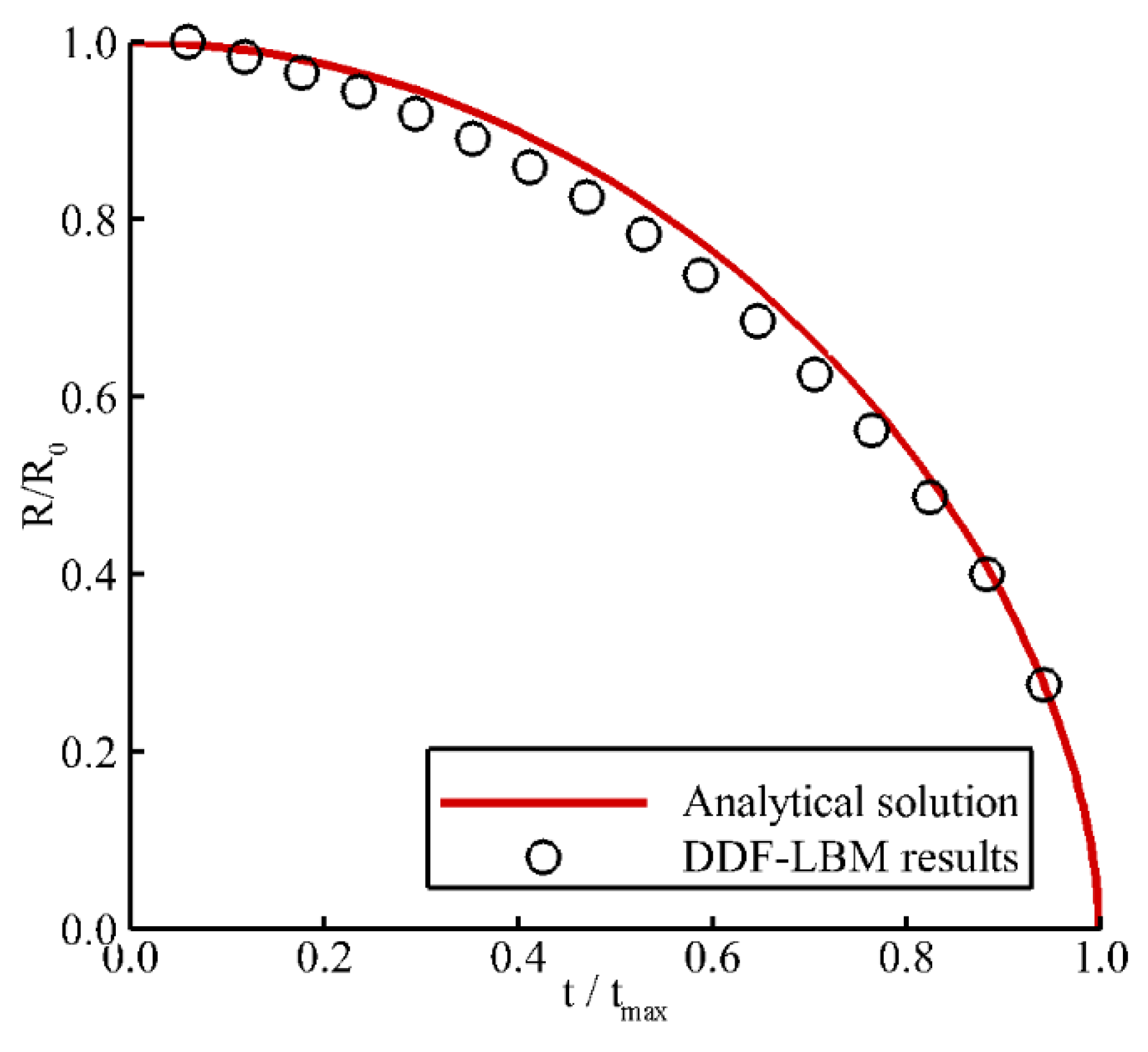
First, the collapse of a bubble in an infinite domain was simulated to verify the used DDF-LBM model. At the beginning, due to the pressure difference between the inside and outside the bubble, the bubble shrinks and then disappears.
In the present simulation, the computational domain is 801 × 801 grids. Table 1 shows the units in the present study:
The temperature unit is dimensionless, and the lattice speed is . The properties of fluid at the interface can be obtained as follows [52]:
where represents or k. The periodic boundary is applied to the four sides. The bubble locates at the center of the domain and shrinks under the pressure difference.
For this case, the modified Rayleigh–Plesset equation [53] can be used to obtain the analytical solutions:
where is the boundary position, denotes the radius of the bubble, and . is the viscosity of fluid. is the surface tension and can be calculated by Laplace’s law. Although the model is non-isothermal, can be obtained by the isothermal model, which does not include the temperature function. The initial bubble radius . The initial temperature , , and the pressure difference . Because the Equation (24) is a second-order equation, another initial condition is required: At , . In all simulations, the diagonal matrix . The parameters in the EOS are set as follows: a = 0.5, b = 1. These parameters are constant in this paper. Because the temperature in the interface between phases is nearly constant, Equation (24) can be solved conveniently by the fourth order Runge–Kutta method.
Figure 1 shows the comparison of the radius evolution between the analytical solution and the results by the DDF-LBM model. It is clear that the collapse processes by the analytical method and DDF-LBM model are basically identical. The bubble radius is equal to 0 at . The results show that the DDF-LBM model can predict cavitation bubble collapse reasonably.
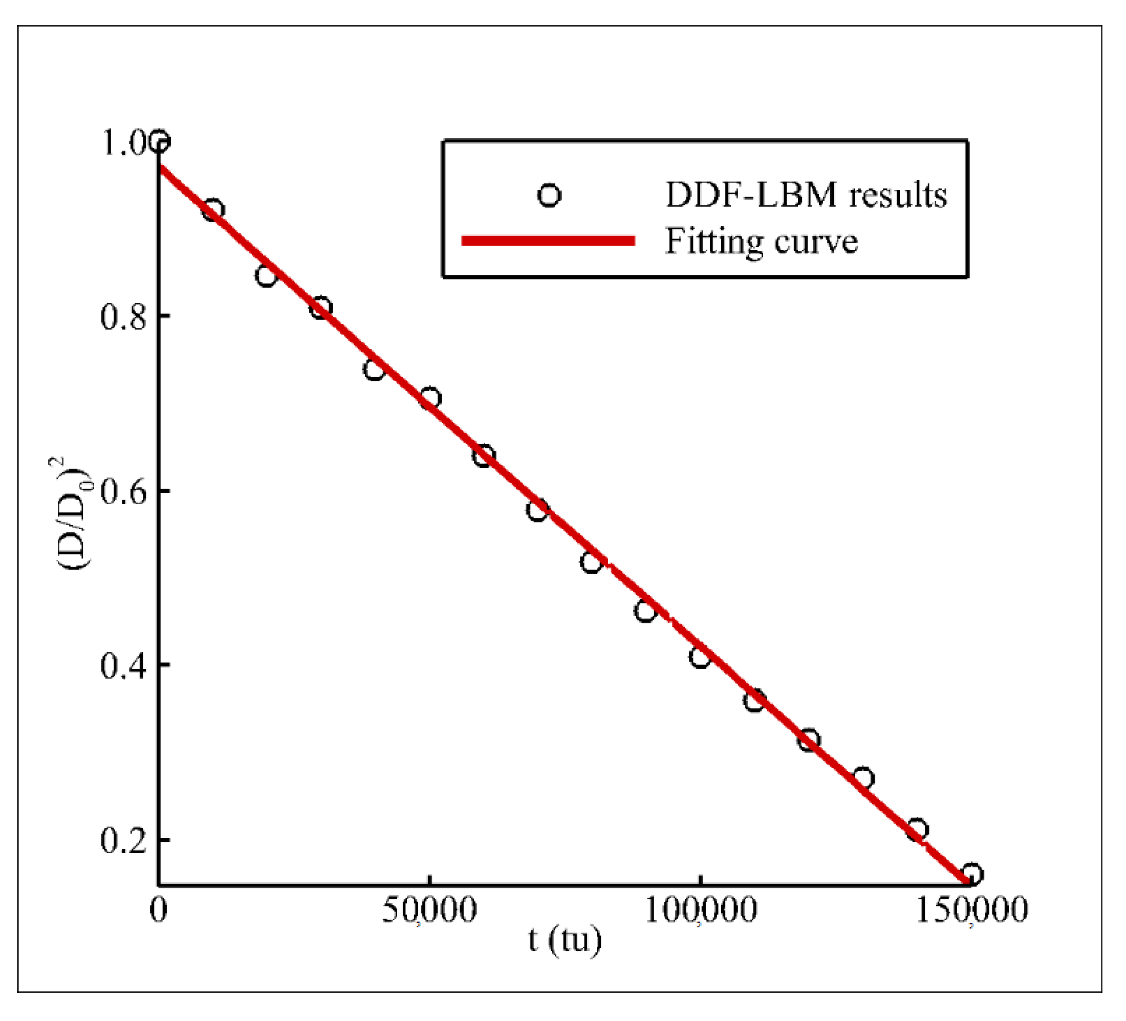
3.2. D2 Law for Droplet Evaporation
Second, the DDF-LBM model was validated further by the D2 (the square of the droplet diameter) law for droplet evaporation in an infinite domain, which indicated that the relationship between the square of the droplet diameter and the time is linear [54]. The law is based on the following assumptions: the liquid and the vapor phases are both quasi-steady; the viscous heat dissipation and buoyancy are neglected. Furthermore, the thermophysical properties are constant, such as k and . In this case, we located the droplet at the center of a domain. The density field can be described by:
where g and l represent the vapor and the liquid, respectively. W represents the width of the interface.
Similarly, the temperature field can be initialized in the same way:
where and are the temperature outside and inside of the bubble in this section, respectively.
In the numerical simulation, the computational domain is 401 × 401 grids. . Due to the temperature difference at the interface between the phases, the droplet evaporation happens. .
Figure 2 shows that the results of the DDF-LBM model are identical to those of the D2 law. However, at the initial stage, there are some errors, which may be because the initial density field is not quasi-steady. Overall, the DDF-LBM model is reliable for the simulation of cavitation.
4. Results and Discussions
After the above verification, three typical cases of cavitation (in an infinite domain, close to a solid wall and a convex wall) were simulated by the improved DDF-LBM model. In the following, the changes of velocity and temperature information during the evolution of the cavitation bubble are discussed in detail.
4.1. Evolution of the Cavitation in an Infinite Domain
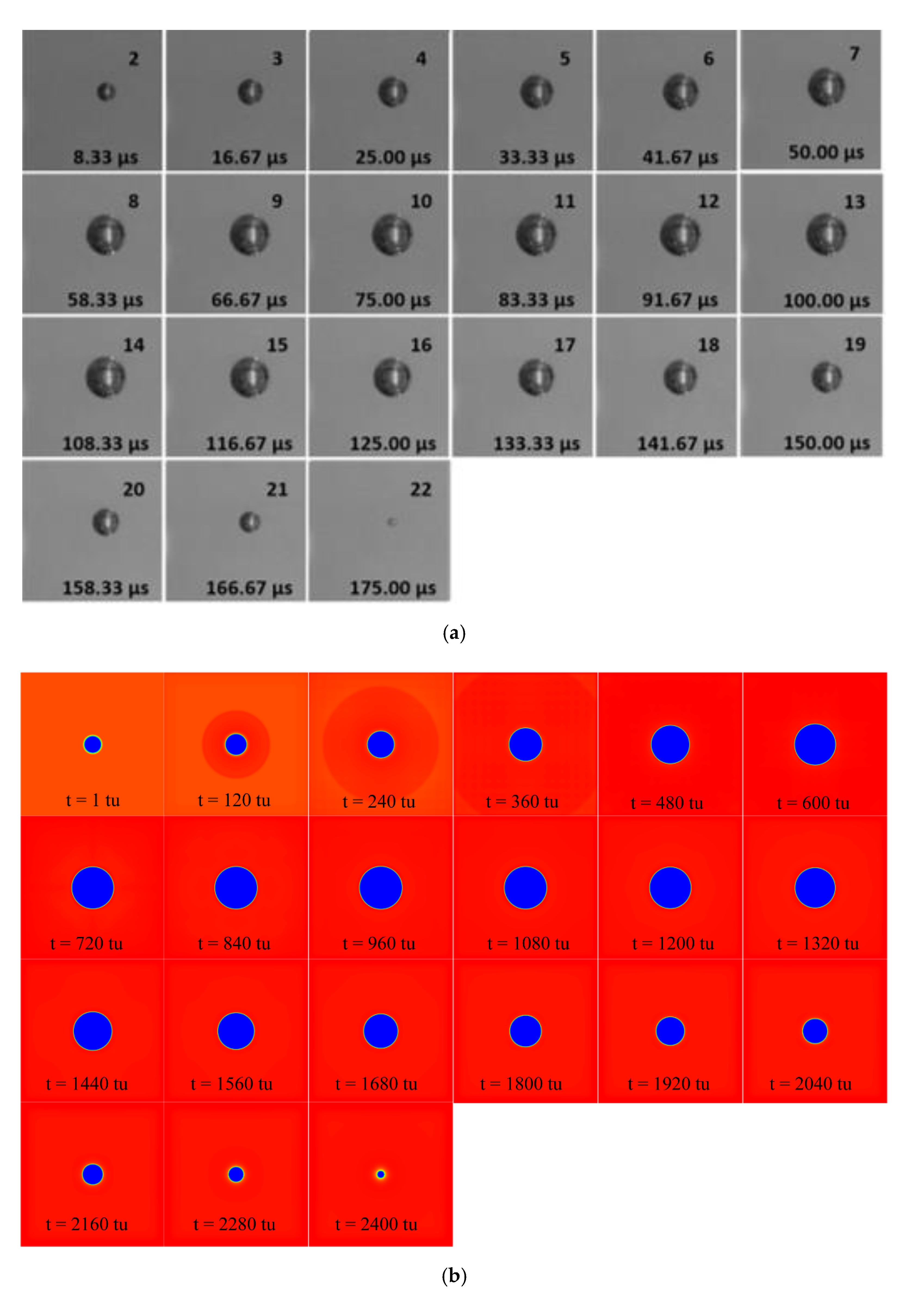
In this section, the evolution of cavitation in an infinite domain is simulated, which includes the growth, the shrinkage and the depression of the cavitation bubble. A square domain was used for the simulation. The periodic boundary is adopted to the four sides. The initial bubble radius , the density field and the temperature field are initialized by Equations (25) and (26), where is 0.42 and 0.0006 , leading to a pressure difference of . and .
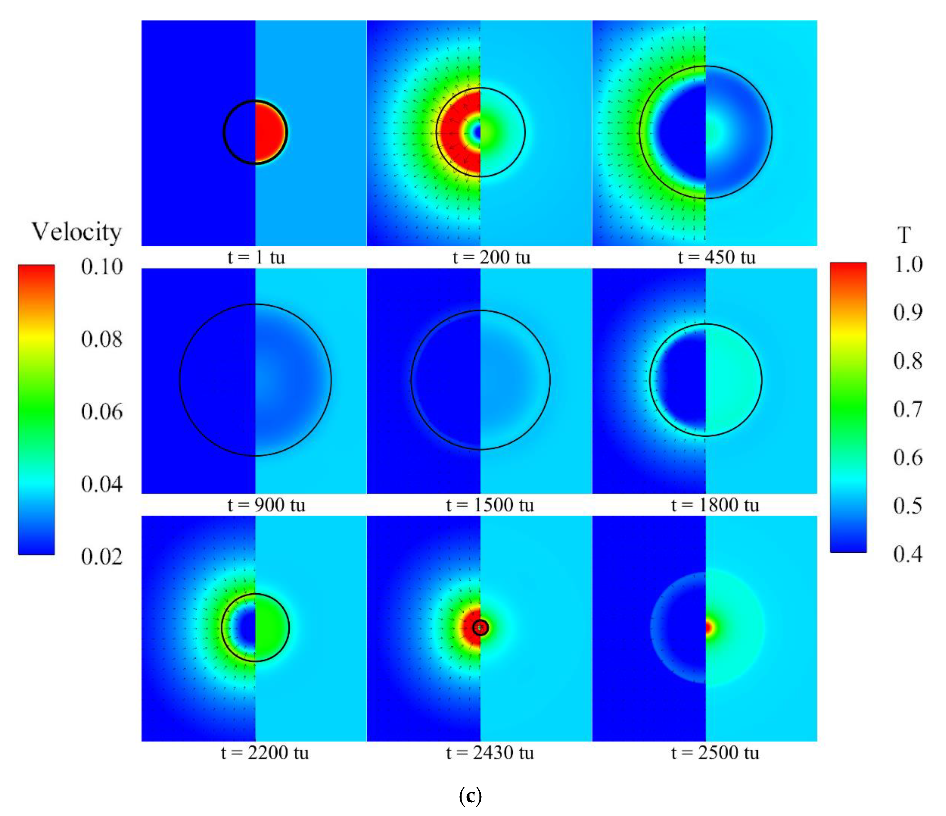
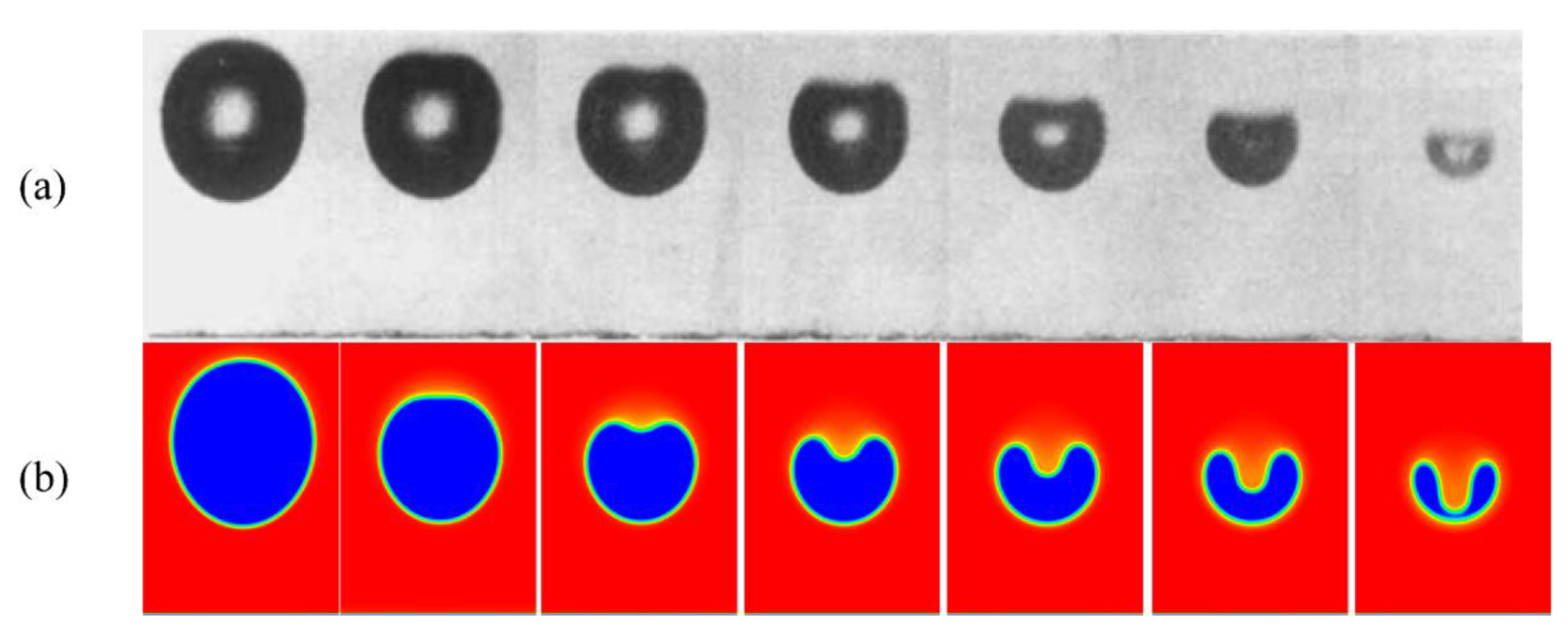
Figure 3 shows the experimental results [55] and simulated results by the DDF-LBM model. It can be found that the simulation by the DDF-LBM model agrees with the experimental results. At first, the bubble expands due to the pressure difference between the inside and outside of the bubble. When the bubble reaches the maximum volume, because the additional pressure at the boundaries transfers to the liquid near the bubble, the ambient pressure is stronger than that in the bubble. So, it starts to shrink and collapse. The results illustrate that there is an obvious different temperature at the surface of the bubble. The temperature field is displayed in Figure 3c. It is clear that the temperature inside the bubble decreases in the process of expansion. Then, it keeps increasing during the shrinkage process and reaches the peak when it collapses.
4.2. Evolution of the Cavitation Near a Straight Wall
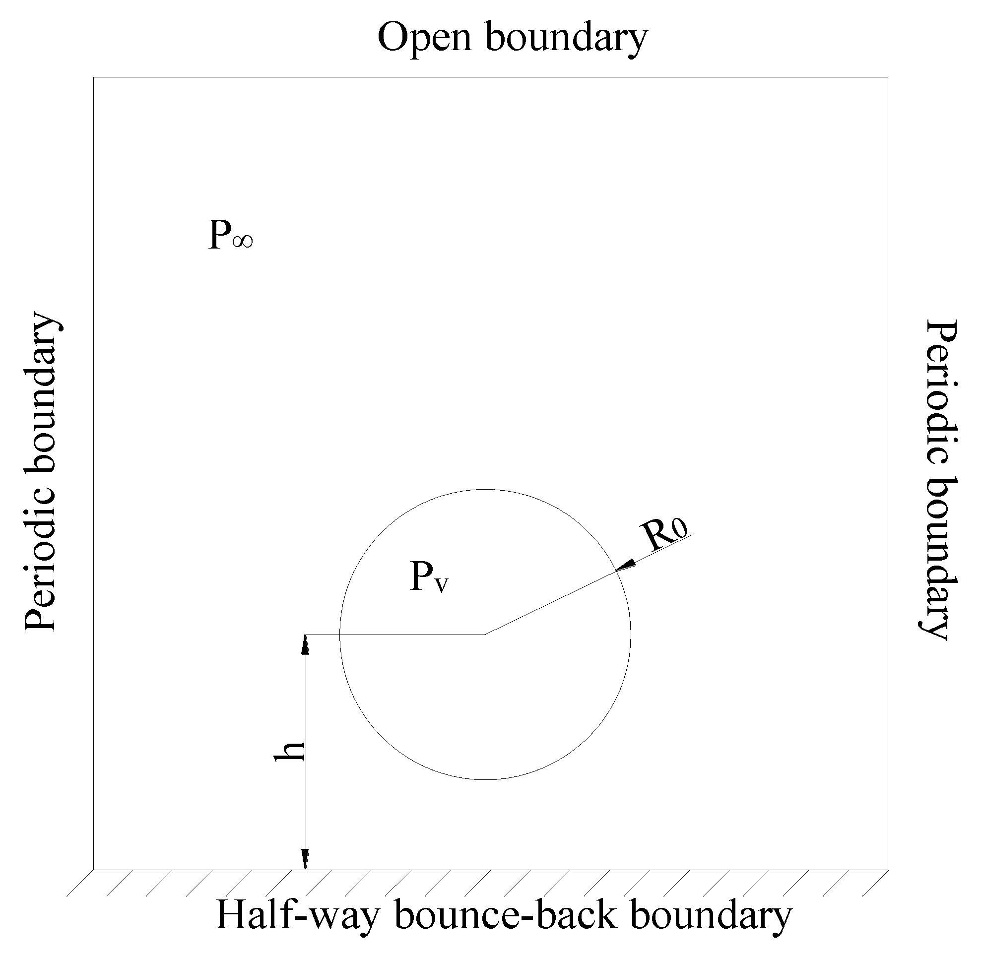
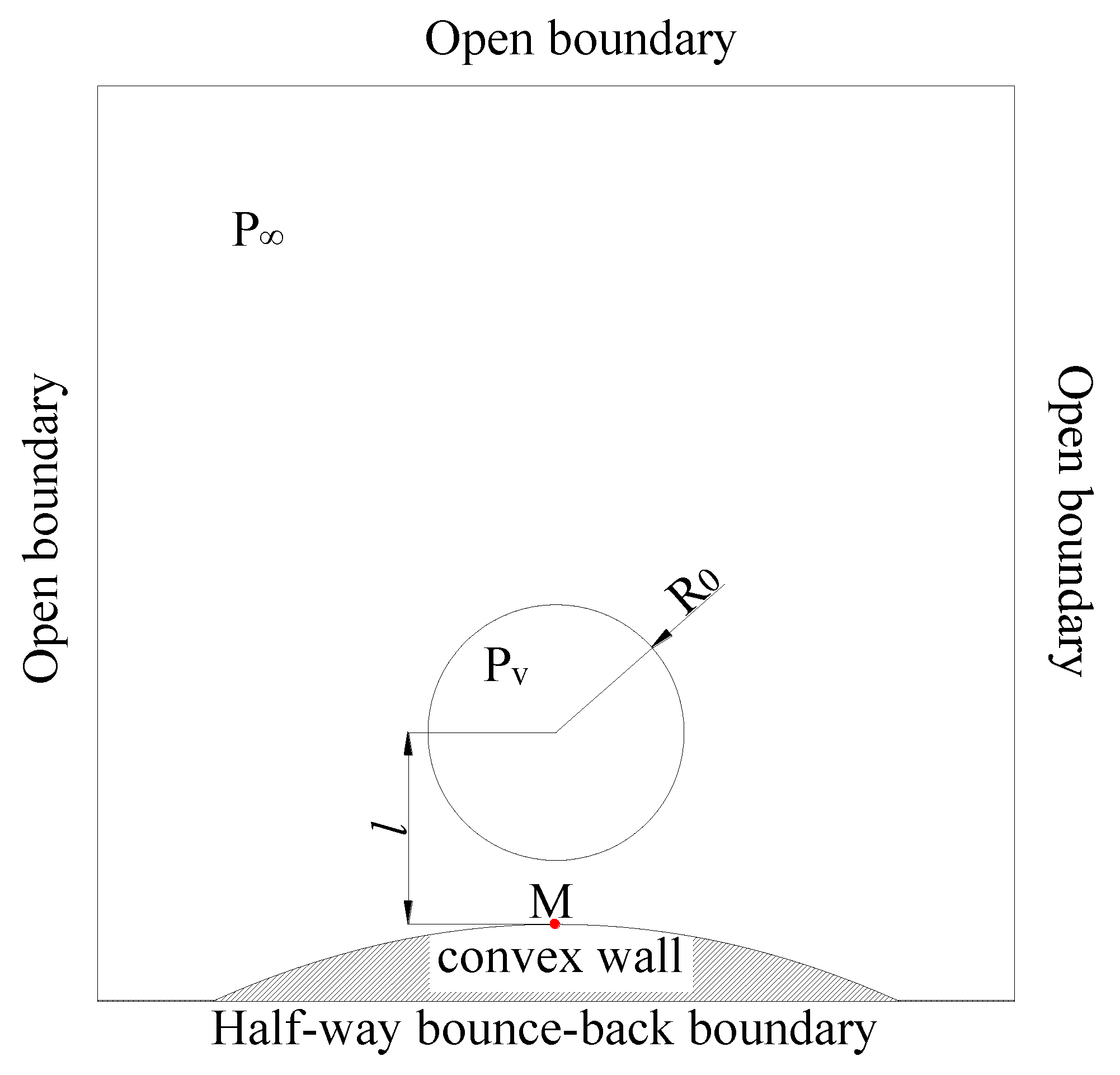
In this section, the evolution of cavitation near a straight wall is discussed in detail. Different from the evolution of the cavitation in an infinite area, the bubbles in this case do not remain spherical when it collapses close to a straight wall. The domain is also set as 501 × 501 . The periodic boundary is adopted for the right and left sides. In addition, the open boundary [56,57,58] is implemented in the top of the domain. A bounce-back [58,59] boundary is applied to the bottom side. The initial bubble radius , the initial density field and the initial temperature field are obtained by the same method; is 0.485 and 0.0006 , . As shown in Figure 4, another parameter is proposed, which represents the distance between the wall and the bubble center.
Figure 5 shows the evolution of the cavitation by the experimental method [60] and the simulation results by the DDF-LBM model when λ = 1.5. The simulation results are identical to the experimental results. At the beginning, due to the pressure difference between the inside and outside of the bubble, the bubble shrinks. The bottom wall of the bubble moves slowly due to the blockage of the wall. Compared to the contraction in the longitudinal direction, the lateral contraction is more obvious, which leads to the bubble shaping into an ellipse. The depression gradually deepens at the upper bubble edge as the pressure difference increases. When the lower bubble edge collides with the upper bubble edge, the collapse occurs.
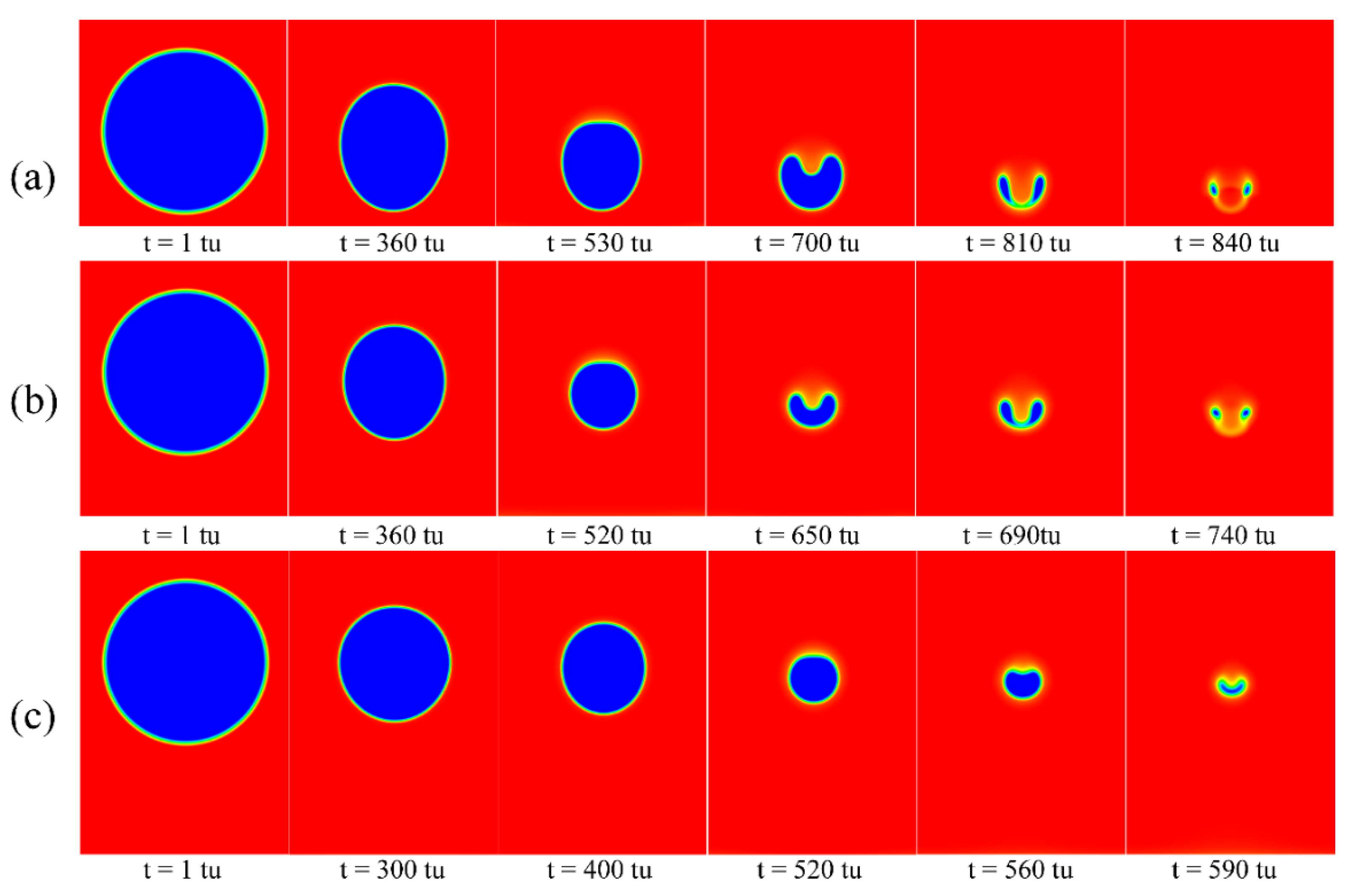
Figure 6 shows the evolution of the cavitation in different positions close to a straight wall. When λ is relatively small (λ = 1.2, 1.8), the evolution process of the bubble is similar to Figure 5. First, it gradually shrinks under the effect of the ambient pressure, and then it collapses and disappears under the pressure generated by the upper boundary. When λ = 2.4, the collapse of the bubble is not consistent with the other two cases. The cavitation bubble shrinks in a spherical shape under the influence of ambient pressure, instead of shrinking into an elliptical shape. The volume of the cavitation bubble is already very small when it begins to depress, and the bubble collapses without a full development of depression. It can be shown from these cases that the bottom edge speed of the bubble gradually increases as λ increases, resulting in a gradual increase in the shrinkage of the bubble, but the occurrence time of the depression is almost the same, so the degree of depression gradually decreases; the cavitation bubble in Figure 6c did not collapse twice.
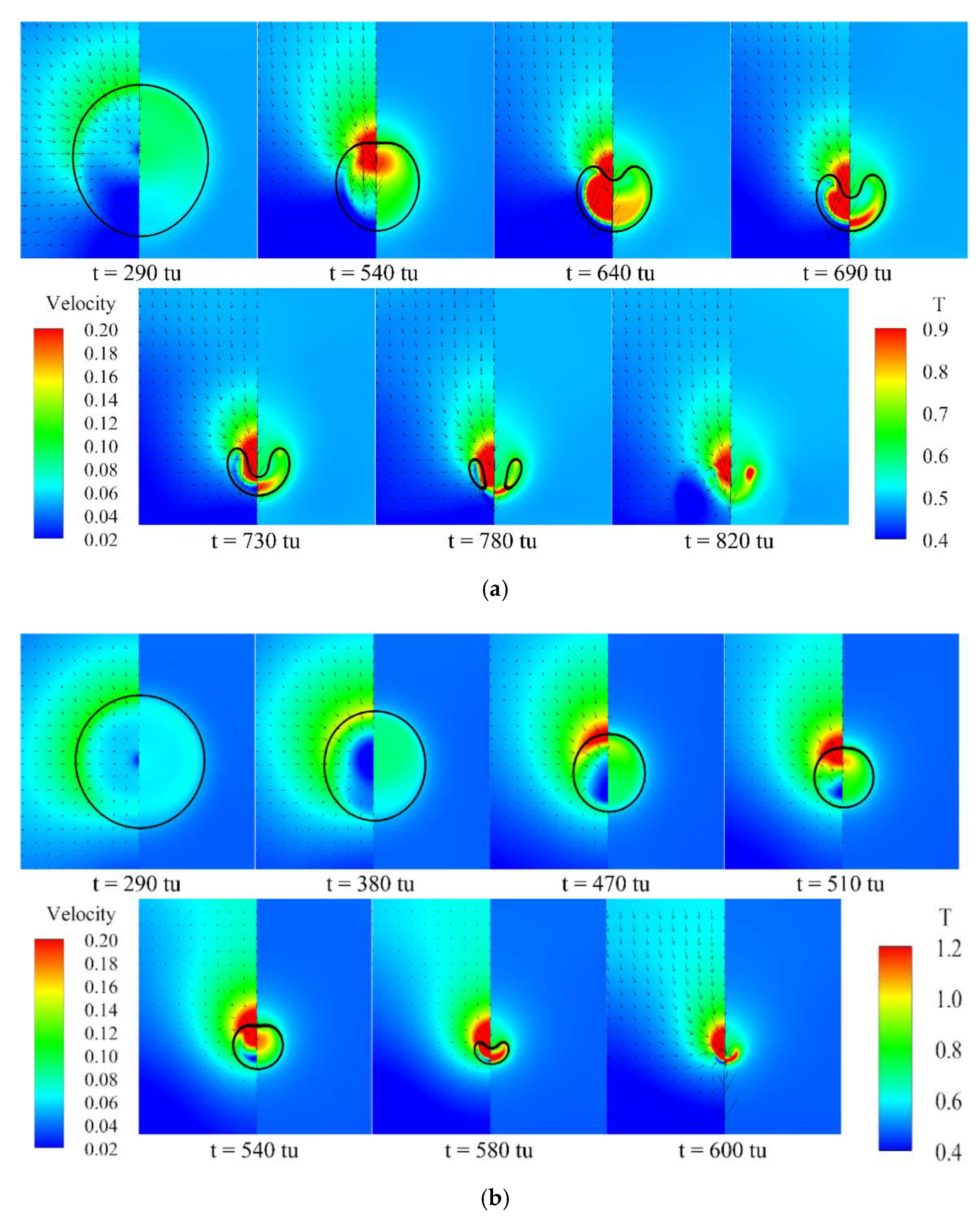
Figure 7 shows the velocity and the temperature fields during the cavitation bubble collapse in different positions. From the previous analysis, it is known that the effect of the wall on bubble reduces with the increase in distance between the bubble and wall, which mainly affects whether the cavitation bubble has secondary collapse or not. It can be seen that the velocity at the bottom of the bubble is nearly zero in Figure 7a because λ is small. As λ increases, the velocity of the cavitation bubble edge also increases, and the maximum velocity appears on the upper edge of the cavitation bubble. As the cavitation bubble continues to shrink, the peak of the temperature inside the bubble also appears in the upper half. When the bubble starts to depress, the velocity of the upper bubble edge increases rapidly. Therefore, the process from cavitation bubble depression to collapse has a short duration, and the location of the highest temperature in the bubble also moves downward. The first collapse produces a pressure wave. With the combined effects of this pressure wave and the micro-jet, the remaining annular bubble eventually collapses. During this process, the location of the highest temperature also moves from the center to the inside of the annular bubble, which is the second collapse.
The bubble in Figure 7b is far from the solid wall. The shape of the bubble during the collapse is different from that in Figure 7a. First, due to the small obstruction by the wall, the lower edge of the bubble has a certain velocity, but it is lower than the velocity of the upper bubble edge. The cavitation bubble shrinks approximately in a spherical shape, and there is a low velocity area in the bubble. As the pressure above the cavitation bubble gradually rises, the velocity of the upper bubble edge gradually increases, and the temperature of the upper portion of the bubble gradually increases, so that a depression appears. Since the volume of the cavitation bubble is already small when it is depressed, it collapses before the depression is fully developed, and there is no second collapse process. In the process of depression, the location of the temperature peak in the bubble gradually moves downward. The reason why there is no second collapse in this case is that λ is large enough, and the lower bubble edge has a certain velocity in the collapse process, so that the micro-jet cannot be fully developed. So, the cavitation bubble disappears during depression.
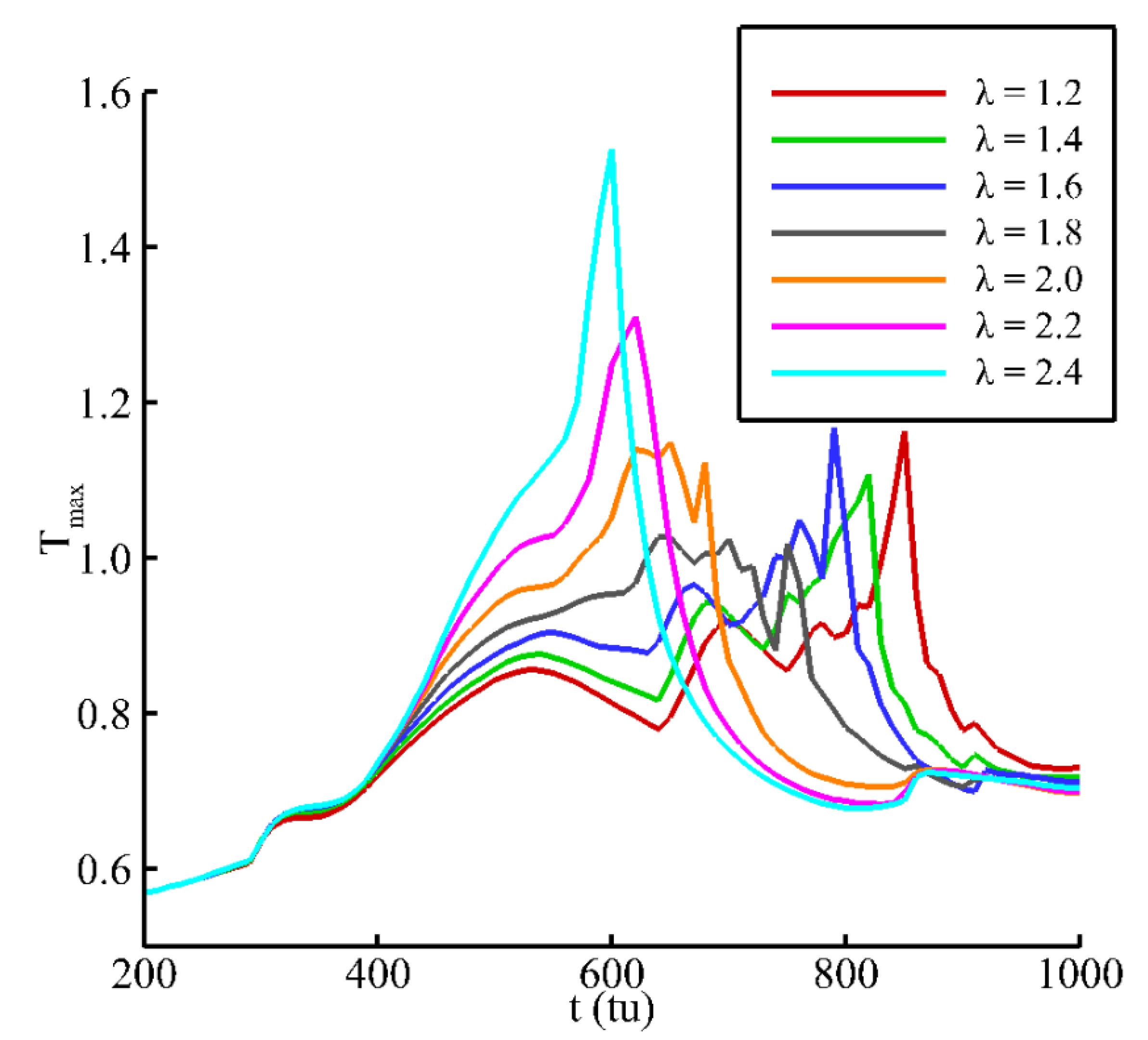
Figure 8 displays the max temperature evolution in different cases. If λ ≥ 2.0, the peak of the temperature increases as the λ increases. It can be found from the Figure 8 that the temperature peak in the cavitation bubble keeps rising during the shrinkage stage. In the depression stage, the temperature changes of various cases are not consistent. When λ < 1.8, the temperature peak of the cavitation bubble in the initial stage of the depression decreases slightly. It can be seen from Figure 7a that the position of the highest temperature in the bubble at this stage gradually moves down, with a small increase. When the position moves to the lower bubble wall, it stops moving downward. During the later period of the depression, the micro-jet has been fully developed, and the compression of the bubble causes the rise in temperature in the bubble. Then, it does not decrease until the second collapse of the cavitation bubble occurs. When λ ≥ 1.8, the maximum temperature in the cavitation bubble shows a trend of increase in the shrinkage and depression stages. Since there is no second collapse, the temperature peak position moves to the lower part.
4.3. Evolution of the Cavitation Near a Convex Wall
In this section, a single cavitation bubble’s growth and collapse near a convex wall is described in detail. In practical engineering, the cavitation often happens near an irregular boundary, so it is vital to investigate the cavitation in complicated boundary conditions. There are also some experiments on cavitation bubble collapse near a convex wall [61], which can be used to verify the simulation. The computational layout for this case is shown in Figure 9. For the density and velocity fields, the open boundary is implemented for the top, right and left boundaries. Additionally, a half-way bounce-back boundary is adopted to the bottom of the domain. As for the temperature field, an isothermal boundary is applied to these four sides. The initial bubble radius is 40 . is 0.422 and 0.0006 , . The computational domain is 501 × 501 grids. The curvature of solid wall is controlled by a function c (x,y) [61]:
where h is the height of the wall, l represents the distance from the bubble center to the wall. is in inverse proportion to the curvature of the wall, which indicates the curvature increase as decreases. The curvature at point M can be defined as [61]: .
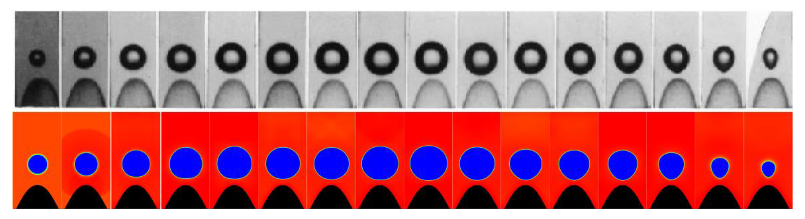
Figure 10 illustrates the evolution of the bubble by experiments [61] and simulation by the DDF-LBM model. It can be shown that the numerical results are identical to those of the experiments. At the beginning, the external pressure of the bubble is lower than the internal pressure. Under this pressure difference, the cavitation bubble expands and grows. After the growth reaches a certain stage, the lower part of the cavitation bubble develops slowly due to the inhibition of the convex wall. When the boundary pressure spreads around the bubble, it begins to shrink. In the shrinking process, compared with the flat wall, the lower bubble edge of the cavitation bubble does not remain smooth, but a sharp corner is evolved. The upper half of the bubble is similar to the shrinking process for the case with a flat wall.
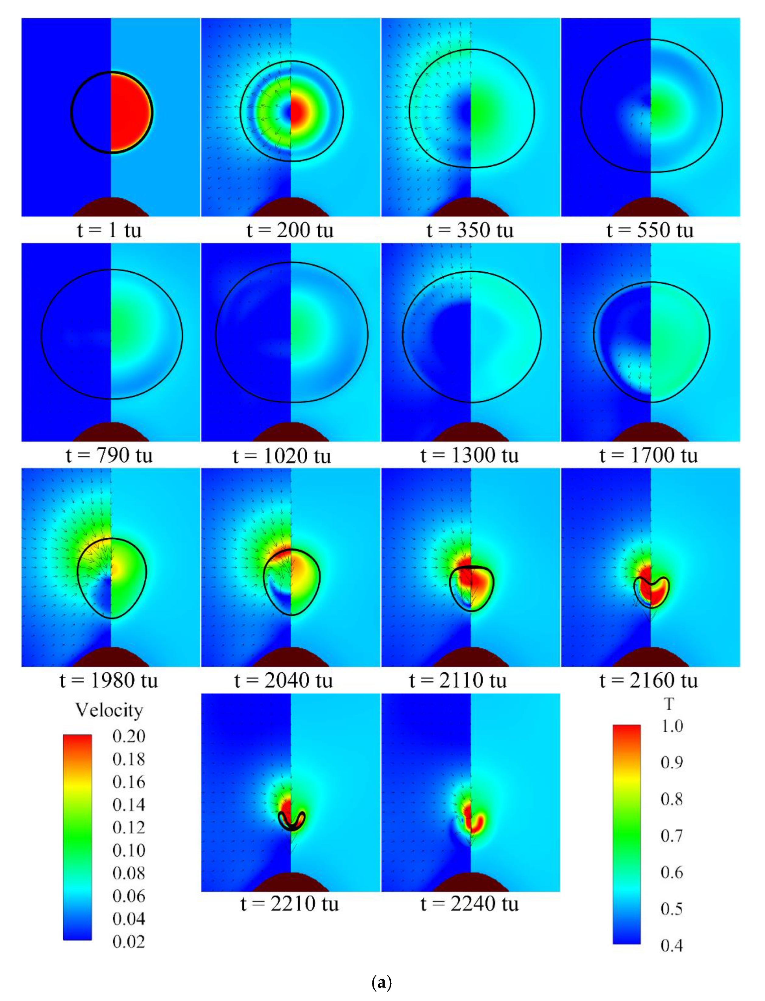
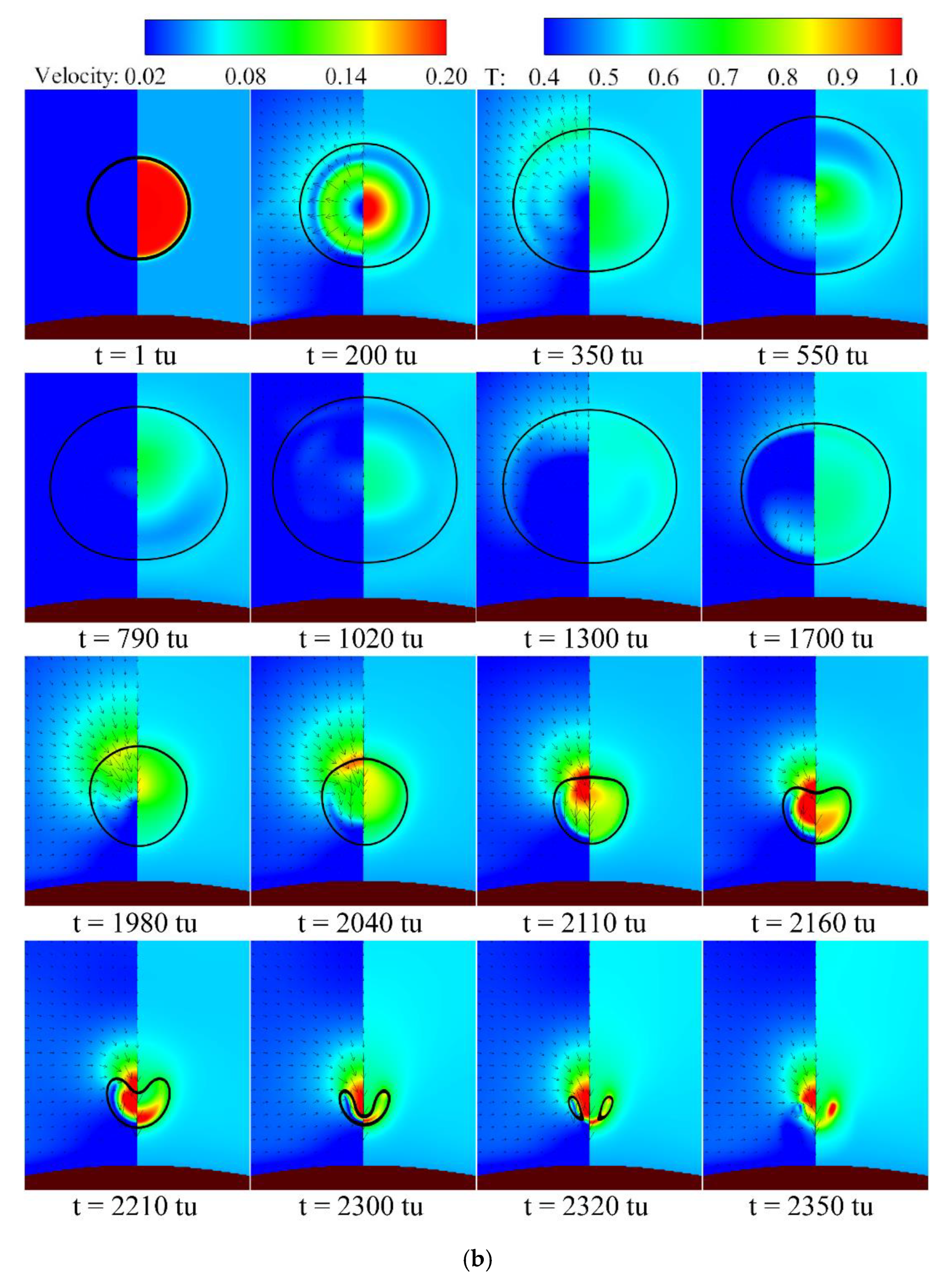
Figure 11 shows the whole process of a bubble’s growth and collapse close to a convex wall with two curvatures. It can be seen that the bubble is basically not affected by the curvature of the wall during the growth stage. The cavitation bubble has a certain outward movement in the initial stage of growth, and the temperature inside the bubble gradually decreases. However, because the lower part of the bubble is suppressed by the wall, it would stop developing when close to the wall. When the boundary pressure spreads around the cavitation bubble, it starts to shrink. Moreover, due to the change of the curvature, the evolution of the velocity of the bubble edge is also different. When the wall curvature is large, in other words, is relatively small, the area occupied by the wall is smaller, resulting in a sharper shape of the lower part of the bubble. However, the velocity of the lower part of the bubble is still lower than that of the upper part. In the initial stage of shrinkage, the location of maximum velocity is always close to the center of the upper bubble wall. In the late stage of shrinkage, it can be found that the upper bubble edge also forms a sharp angle, and the maximum velocity appears on both sides of the upper bubble edge. The bubble temperature continues to rise during the shrinking process. If the curvature is small, the area affected by the wall becomes larger, and the velocity of the lower part of the cavitation bubble becomes smaller, so there is no obvious sharp corner. During the depression of the cavitation bubble, the top edge speed increases sharply, the temperature inside the bubble also increases and the position of peak temperature moves downward accordingly. It can be seen that if the curvature is small, the second collapse occurs. However, if the curvature is large, the lower sharp corner is obvious, and the second collapse does not exist.
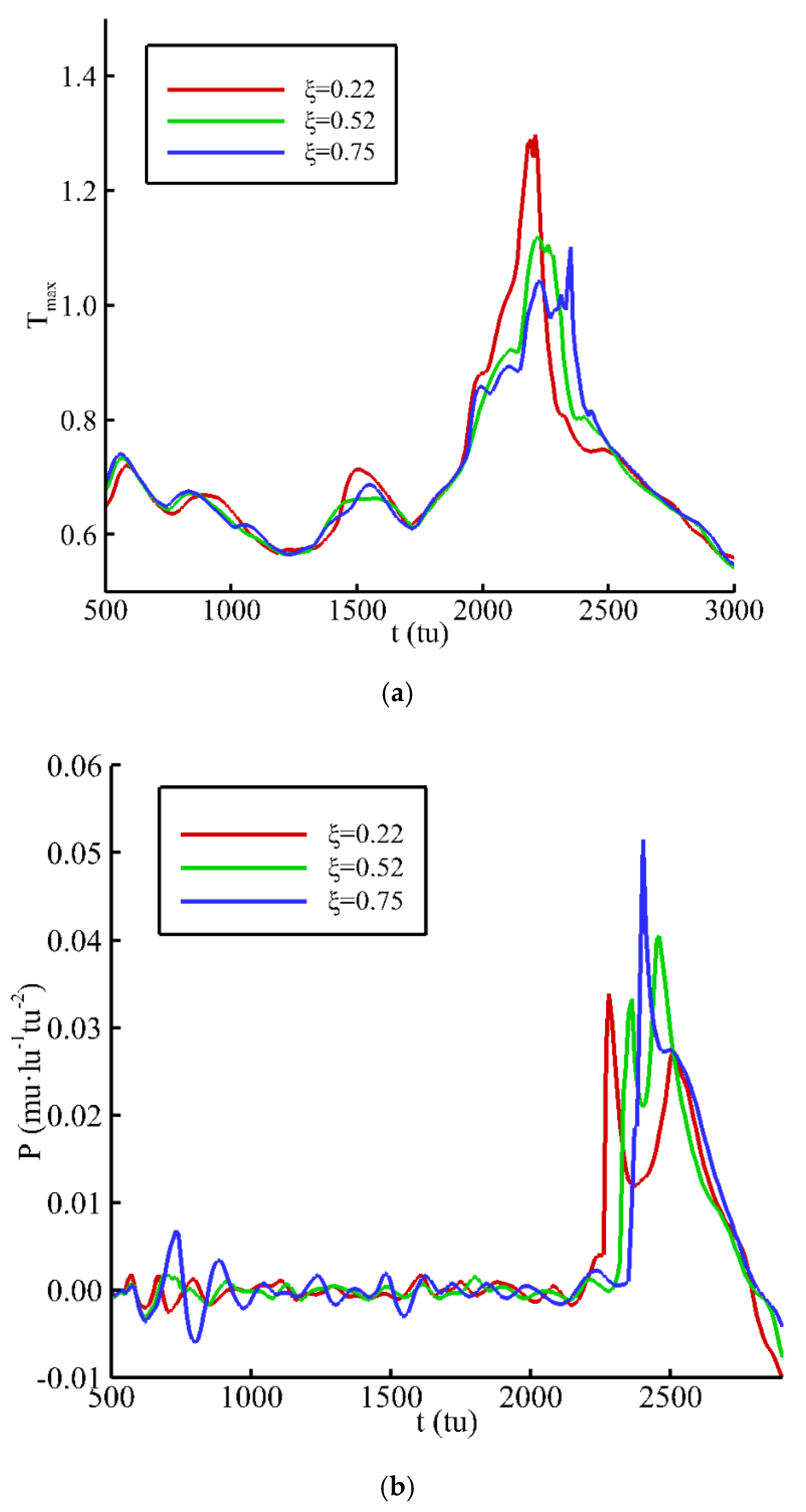
Figure 12 shows the evolution of the maximum temperature inside the bubble and the change of pressure in the center of the convex wall during the growth and collapse processes of the cavitation bubble under different curvatures. During the growth stage of the cavitation bubble, the maximum temperature in the bubble shows some fluctuations to a certain extent, but it is close to the ambient temperature. When the bubble starts to shrink, the highest temperature inside the bubble rises sharply, and reaches the extremum when it collapses. Among these three cases, the largest temperature appears in the case. In this case, compared to the lower part, the bubble has a larger velocity on the upper part of the bubble. The compression speed of the bubble is the fastest. The pressure at the center of the convex wall is close to 0 before the collapse of the bubble. When the pressure wave induced by collapse reaches the wall, the pressure increases sharply. The maximum pressure on the convex wall comes from the case. This is because the cavitation bubble has a second collapse, and the time between the two collapses is short. The pressure waves generated by the two collapses superimpose and impact the convex wall.
5. Conclusions
In this study, an improved DDF-LBM model was applied for the simulation of the non-isothermal cavitation. The density and velocity fields were simulated by the pseudo-potential model, and the temperature field was simulated by the thermal LBM model. After the proposed LBM model was verified, it was used to study the cavitation bubble collapse in three typical boundaries, namely, an infinite domain, a straight wall and a convex wall. In view of the simulation, the following conclusion can be obtained:
- (1)
- The LBM model successfully reproduces the process from the expansion to compression of the cavitation bubble for the case of an infinite domain. In the initial growth stage, the temperature inside the bubble decreases, and the high pressure and the temperature are found at the final collapse stage due to the bubble compression.
- (2)
- When a cavitation bubble is near the straight wall, λ determines whether the second collapse exists or not. During the shrinkage stage, the temperature inside the bubble keeps rising, and the position of the maximum temperature in the bubble moves downwards in the depression stage. If the second collapse exists, the temperature inside the bubble has a slight fluctuation during the depression stage and the position of the maximum temperature has lateral movement following the annular bubble after the first collapse. When λ is large enough (λ = 2.2, 2.4), the temperature inside the bubble is obviously higher compared with the other cases.
- (3)
- When a bubble is near a convex wall, the curvature of the wall can affect the behavior of the bubble collapse. In the shrinkage stage, the lower edge of the bubble evolves into a sharp corner due to the compression of both sides of the bubble’s lower part for the case of . However, the sharp corner does not exist when , and the bubble has a second collapse, which is similar to the bubble near the straight wall. However, the temperature for the case of in the evolution is the largest. When , the pressure at the center of the convex wall is the largest, which indicates that the wall pressure reduces as the decreases.
- (4)
- Overall, the improved LBM model can accurately predict cavitation bubble collapse, including the heat transfer. Moreover, the interaction between density and temperature fields has been included in the LBM model for the first time.
Author Contributions
Conceptualization, Y.P.; methodology, Y.P.; software, Y.L.; validation, Y.L.; writing—original draft preparation, Y.L.; writing—review and editing, Y.P.; supervision, Y.P.; project administration, Y.P.; funding acquisition, Y.P. All authors have read and agreed to the published version of the manuscript.
Funding
This research was funded by the National Natural Science Foundation of China, grant number 51979184& 51579166; the Science and Technology Department of Sichuan Province, grant number 2019YJ0121; and the State Key Laboratory of Hydraulics and Mountain River Engineering, grant number SKHL1905&SKHL2005.
Institutional Review Board Statement
Not applicable.
Informed Consent Statement
Not applicable.
Data Availability Statement
“MDPI Research Data Policies” at https://0-www-mdpi-com.brum.beds.ac.uk/ethics.
Acknowledgments
The authors thank the National Natural Science Foundation of China (Project No: 51979184, 51579166), the Science and Technology Department of Sichuan Province (Project No: 2019YJ0121), and the State Key Laboratory of Hydraulics and Mountain River Engineering (Open Fund No: SKHL1905 and SKHL2005) for their financial support.
Conflicts of Interest
The authors declare no conflict of interest.
References
- Brennen, C.; Acosta, A.J. The Dynamic Transfer Function for a Cavitating Inducer. J. Fluids Eng. 1976, 98, 182–191. [Google Scholar] [CrossRef]
- Kornfeld, M.; Suvorov, L. On the Destructive Action of Cavitation. J. Appl. Phys. 1944, 15, 495–506. [Google Scholar] [CrossRef]
- Ohl, S.-W.; Wu, D.W.; Klaseboer, E.; Khoo, B.C. Spark bubble interaction with a suspended particle. J. Phys. Conf. Ser. 2015, 656, 012033. [Google Scholar] [CrossRef] [Green Version]
- Poulain, S.; Guenoun, G.; Gart, S.; Crowe, W.; Jung, S. Particle Motion Induced by Bubble Cavitation. Phys. Rev. Lett. 2015, 114, 214501. [Google Scholar] [CrossRef] [Green Version]
- Vogel, A.; Lauterborn, W. Acoustic transient generation by laser-produced cavitation bubbles near solid boundaries. J. Acoust. Soc. Am. 1988, 84, 719–731. [Google Scholar] [CrossRef]
- Tomita, Y.; Kodama, T. Interaction of laser-induced cavitation bubbles with composite surfaces. J. Appl. Phys. 2003, 94, 2809–2816. [Google Scholar] [CrossRef]
- Huang, S.; Ihara, A.; Watanabe, H.; Hashimoto, H. Effects of Solid Particle Properties on Cavitation Erosion in Solid-Water Mixtures. J. Fluids Eng. 1996, 118, 749–755. [Google Scholar] [CrossRef]
- Arora, M.; Ohl, C.D.; Mørch, K.A. Cavitation Inception on Microparticles: A Self-Propelled Particle Accelerator. Phys. Rev. Lett. 2004, 92, 174501. [Google Scholar] [CrossRef] [Green Version]
- Naude, C.F.; Ellis, A.T. On the Mechanism of Cavitation Damage by Nonhemispherical Cavities Collapsing in Contact with a Solid Boundary. J. Basic Eng. 1961, 83, 648–656. [Google Scholar] [CrossRef]
- Kling, C.L.; Hammitt, F.G. A Photographic Study of Spark-Induced Cavitation Bubble Collapse. J. Basic Eng. 1972, 94, 825–832. [Google Scholar] [CrossRef]
- Vogel, A.; Lauterborn, W.; Timm, R. Optical and acoustic investigations of the dynamics of laser-produced cavitation bubbles near a solid boundary. J. Fluid Mech. 1989, 206, 299–338. [Google Scholar] [CrossRef]
- Dular, M.; Coutier-Delgosha, O. Thermodynamic effects during growth and collapse of a single cavitation bubble. J. Fluid Mech. 2013, 736, 44–66. [Google Scholar] [CrossRef] [Green Version]
- Popinet, S.; Zaleski, S. Bubble collapse near a solid boundary: A numerical study of the influence of viscosity. J. Fluid Mech. 2002, 464, 137–163. [Google Scholar] [CrossRef] [Green Version]
- Shan, X.W.; Chen, H.D. Lattice Boltzmann model for simulating flows with multiple phases and components. Phys. Rev. E 1993, 47, 1815–1819. [Google Scholar] [CrossRef] [PubMed] [Green Version]
- Chen, S.Y.; Doolen, G.D. Lattice Boltzmann Method for Fluid Flows. Annu. Rev. Fluid Mech. 1998, 30, 329–364. [Google Scholar] [CrossRef] [Green Version]
- d’Humières, D. Generalized Lattice-Boltzmann Equations. In Proceedings of the 18th International Symposium on Rarefied Gas Dynamics, Vancouver, BC, Canada, 26–30 July 1992; pp. 450–458. [Google Scholar]
- Li, Q.; Luo, K.H.; Li, X.J. Lattice Boltzmann modeling of multiphase flows at large density ratio with an improved pseudopotential model. Phys. Rev. E 2013, 87, 053301. [Google Scholar] [CrossRef] [PubMed] [Green Version]
- Sankaranarayanan, K.; Shan, X.; Kevrekidis, I.; Sundaresan, S. Bubble flow simulations with the lattice Boltzmann method. Chem. Eng. Sci. 1999, 54, 4817–4823. [Google Scholar] [CrossRef]
- Sukop, M.C.; Or, D. Lattice Boltzmann method for homogeneous and heterogeneous cavitation. Phys. Rev. E 2005, 71, 046703. [Google Scholar] [CrossRef]
- Mishra, S.K.; Deymier, P.A.; Muralidharan, K.; Frantziskonis, G.; Pannala, S.; Simunovic, S. Modeling the coupling of reaction kinetics and hydrodynamics in a collapsing cavity. Ultrason. Sonochem. 2010, 17, 258–265. [Google Scholar] [CrossRef]
- Shan, M.-L.; Zhu, C.-P.; Yao, C.; Yin, C.; Jiang, X.-Y. Pseudopotential multi-relaxation-time lattice Boltzmann model for cavitation bubble collapse with high density ratio. Chin. Phys. B 2016, 25, 104701. [Google Scholar] [CrossRef]
- Su, Y.; Tang, X.; Wang, F.; Li, X.; Shi, X. Three-Dimensional Cavitation Bubble Simulations based on Lattice Boltzmann Model Coupled with Carnahan-Starling Equation of State. Commun. Comput. Phys. 2017, 22, 473–493. [Google Scholar] [CrossRef]
- Mao, Y.F.; Peng, Y.; Zhang, J.M. Study of Cavitation Bubble Collapse near a Wall by the Modified Lattice Boltzmann Method. Water 2018, 10, 1439. [Google Scholar] [CrossRef] [Green Version]
- Peng, C.; Tian, S.; Li, G.; Sukop, M.C. Simulation of multiple cavitation bubbles interaction with single-component multiphase Lattice Boltzmann method. Int. J. Heat Mass Transf. 2019, 137, 301–317. [Google Scholar] [CrossRef]
- Liu, Y.; Yong, P. Study on the Collapse Process of Cavitation Bubbles near the Concave Wall by Lattice Boltzmann Method Pseudo-Potential Model. Energies 2020, 13, 4398. [Google Scholar] [CrossRef]
- Márkus, A.; Házi, G. Simulation of evaporation by an extension of the pseudopotential lattice Boltzmann method: A quantitative analysis. Phys. Rev. E 2011, 83, 046705. [Google Scholar] [CrossRef]
- Gong, S.; Cheng, P. Lattice Boltzmann simulation of periodic bubble nucleation, growth and departure from a heated surface in pool boiling. Int. J. Heat Mass Transf. 2013, 64, 122–132. [Google Scholar] [CrossRef]
- Safari, H.; Rahimian, M.H.; Krafczyk, M. Consistent simulation of droplet evaporation based on the phase-field multiphase lattice Boltzmann method. Phys. Rev. E 2014, 90, 033305. [Google Scholar] [CrossRef]
- Li, Q.; Kang, Q.J.; Francois, M.; He, Y.L.; Luo, K.H. Lattice Boltzmann modeling of boiling heat transfer: The boiling curve and the effects of wettability. Int. J. Heat Mass Transf. 2015, 85, 787–796. [Google Scholar] [CrossRef] [Green Version]
- Gonnella, G.; Lamura, A.; Sofonea, V. Lattice Boltzmann simulation of thermal nonideal fluids. Phys. Rev. E 2007, 76, 036703. [Google Scholar] [CrossRef] [Green Version]
- Gan, Y.; Xu, A.; Zhang, G.; Succi, S. Discrete Boltzmann modeling of multiphase flows: Hydrodynamic and thermodynamic non-equilibrium effects. Soft Matter 2015, 11, 5336–5345. [Google Scholar] [CrossRef] [Green Version]
- Shan, X. Simulation of Rayleigh-Bénard convection using a lattice Boltzmann method. Phys. Rev. E 1997, 55, 2780–2788. [Google Scholar] [CrossRef] [Green Version]
- He, X.Y.; Chen, S.Y.; Doolen, G.D. A Novel Thermal Model for the Lattice Boltzmann Method in Incompressible Limit. J. Comput. Phys. 1998, 146, 282–300. [Google Scholar] [CrossRef]
- Guo, Z.L.; Shi, B.C.; Zheng, C.G. A coupled lattice BGK model for the Boussinesq equations. Int. J. Numer. Method. Fluid. 2002, 39, 325–342. [Google Scholar] [CrossRef]
- Guo, Z.; Zheng, C.; Shi, B.; Zhao, T.S. Thermal lattice Boltzmann equation for low Mach number flows: Decoupling model. Phys. Rev. E 2007, 75, 036704. [Google Scholar] [CrossRef]
- Lallemand, P.; Luo, L.S. Hybrid Finite-Difference Thermal Lattice Boltzmann Equation. Int. J. Mod. Phys. B 2003, 17, 41–47. [Google Scholar] [CrossRef]
- Peng, C.; Tian, S.; Li, G.; Sukop, M.C. Simulation of laser-produced single cavitation bubbles with hybrid thermal Lattice Boltzmann method. Int. J. Heat Mass Transf. 2020, 149, 119136. [Google Scholar] [CrossRef]
- Yang, Y.; Shan, M.; Kan, X.; Shangguan, Y.; Han, Q. Thermodynamic of collapsing cavitation bubble investigated by pseudopotential and thermal MRT-LBM. Ultrason. Sonochem. 2020, 62, 104873. [Google Scholar] [CrossRef]
- Li, Q.; Zhou, P.; Yan, H.J. Improved thermal lattice Boltzmann model for simulation of liquid-vapor phase change. Phys. Rev. E 2017, 96, 063303. [Google Scholar] [CrossRef] [Green Version]
- Mukherjee, S.; Abraham, J. A pressure-evolution-based multi-relaxation-time high-density-ratio two-phase lattice-Boltzmann model. Comput. Fluids 2007, 36, 1149–1158. [Google Scholar] [CrossRef]
- Lallemand, P.; Luo, L.S. Theory of the lattice Boltzmann method: Dispersion, dissipation, isotropy, Galilean invariance, and stability. Phys. Rev. E 2000, 61, 6546–6562. [Google Scholar] [CrossRef] [Green Version]
- Mohamad, A.A. Lattice Boltzmann Method: Fundamentals and Engineering Applications with Computer Codes; Springer: New York, NY, USA, 2011; ISBN 978-1-4471-7423-3. [Google Scholar]
- Li, Q.; He, Y.L.; Tang, G.H.; Tao, W.Q. Improved axisymmetric lattice Boltzmann scheme. Phys. Rev. E 2010, 81, 056707. [Google Scholar] [CrossRef] [Green Version]
- Shan, X.W. Analysis and reduction of the spurious current in a class of multiphase lattice Boltzmann models. Phys. Rev. E 2006, 73, 047701. [Google Scholar] [CrossRef] [PubMed]
- Shan, X.W. Pressure tensor calculation in a class of nonideal gas lattice Boltzmann models. Phys. Rev. E 2008, 77, 066702. [Google Scholar] [CrossRef]
- Sbragaglia, M.; Benzi, R.; Biferale, L.; Succi, S.; Sugiyama, K.; Toschi, F. Generalized lattice Boltzmann method with multirange pseudopotential. Phys. Rev. E 2007, 75, 026702. [Google Scholar] [CrossRef] [PubMed] [Green Version]
- Li, Q.; Luo, K.H.; Kang, Q.J.; Chen, Q. Contact angles in the pseudopotential lattice Boltzmann modeling of wetting. Phys. Rev. E 2014, 90, 053301. [Google Scholar] [CrossRef] [PubMed] [Green Version]
- Yuan, P.; Schaefer, L. Equations of state in a lattice Boltzmann model. Phys. Fluids 2006, 18, 042101. [Google Scholar] [CrossRef]
- Sedov, L.I. Mechanics of Continuous Media; World Scientific: Singapore, 1997; ISBN 978-981-279-711-7. [Google Scholar]
- Ershkov, S.; Leshchenko, D.; Giniyatullin, A.R. Note on the solving the Laplace tidal equation with linear dissipation. Rom. J. Phys. 2020, 65, 110. [Google Scholar]
- Huang, R.Z.; Wu, H.Y. A modified multiple-relaxation-time lattice Boltzmann model for convection–diffusion equation. J. Comput. Phys. 2014, 274, 50–63. [Google Scholar] [CrossRef] [Green Version]
- Chen, X.P. Simulation of 2D Cavitation Bubble Growth under Shear Flow by Lattice Boltzmann Model. Commun. Comput. Phys. 2010, 7, 212–223. [Google Scholar] [CrossRef]
- Gong, S.; Cheng, P. A lattice Boltzmann method for simulation of liquid–vapor phase-change heat transfer. Int. J. Heat Mass Transf. 2012, 55, 4923–4927. [Google Scholar] [CrossRef]
- Law, C.K. Recent advances in droplet vaporization and combustion. Prog. Energy Combus. Sci. 1982, 8, 171–201. [Google Scholar] [CrossRef]
- Zhang, Y.N.; Chen, F.P.; Zhang, Y.N.; Zhang, Y.; Du, X. Experimental investigations of interactions between a laser-induced cavitation bubble and a spherical particle. Exp. Therm. Fluid Sci. 2018, 98, 645–661. [Google Scholar] [CrossRef]
- Ginzburg, I.; Verhaeghe, F.; d’Humières, D. Study of Simple Hydrodynamic Solutions with the Two-Relaxation-Times Lattice Boltzmann Scheme. Commu. Comput. Phys. 2008, 3, 519–581. [Google Scholar]
- Izquierdo, S.; Fueyo, N. Characteristic nonreflecting boundary conditions for open boundaries in lattice Boltzmann methods. Phys. Rev. E 2008, 78, 046707. [Google Scholar] [CrossRef] [PubMed] [Green Version]
- Krüger, T.; Kusumaatmaja, H.; Kuzmin, A.; Shardt, O.; Silva, G.; Viggen, E.M. The Lattice Boltzmann Method: Principles and Practice; Springer: New York, NY, USA, 2016; ISBN 978-3-3194-4649-3. [Google Scholar]
- Ladd, A.J.C. Numerical simulations of particulate suspensions via a discretized Boltzmann equation. Part 1. Theoretical foundation. J. Fluid Mech. 1994, 271, 285–309. [Google Scholar] [CrossRef] [Green Version]
- Lauterborn, W.; Bolle, H. Experimental investigations of cavitation-bubble collapse in the neighbourhood of a solid boundary. J. Fluid Mech. 1975, 72, 391–399. [Google Scholar] [CrossRef]
- Tomita, Y.; Robinson, P.B.; Tong, R.P.; Blake, J.R. Growth and collapse of cavitation bubbles near a curved rigid boundary. J. Fluid Mech. 2002, 466, 259–283. [Google Scholar] [CrossRef]
Figure 1.
Comparison of the radius evolution between analytical solution and the results by DDF-LBM model.
Figure 1.
Comparison of the radius evolution between analytical solution and the results by DDF-LBM model.

Figure 2.
Validation of the D2 (the square of the droplet diameter) law by DDF–LBM model.

Figure 3.
The evolution of single cavitation bubble in an infinite domain. (a) Experimental results [55], reproduced or adapted from adequate reference, with permission from publisher Elsevier, 2021; (b) density field obtained by the DDF-LBM model; (c) velocity and the temperature fields by DDF-LBM model.


Figure 4.
Computational layout for the cavitation bubble collapse near a straight wall.

Figure 5.
Comparison of experimental data and numerical results by DDF-LBM model. (a) Experimental data [60], reproduced or adapted from adequate reference, with permission from publisher Cambridge University Press, 2021. (b) Simulation results.
Figure 5.
Comparison of experimental data and numerical results by DDF-LBM model. (a) Experimental data [60], reproduced or adapted from adequate reference, with permission from publisher Cambridge University Press, 2021. (b) Simulation results.

Figure 6.
Cavitation bubble collapse in different positions by DDF-LBM model. (a) λ = 1.2; (b) λ = 1.8; (c) λ = 2.4.
Figure 6.
Cavitation bubble collapse in different positions by DDF-LBM model. (a) λ = 1.2; (b) λ = 1.8; (c) λ = 2.4.

Figure 7.
The predicted velocity and the temperature fields of bubble collapse process with different positions. (a) λ = 1.4; (b) λ = 2.4.
Figure 7.
The predicted velocity and the temperature fields of bubble collapse process with different positions. (a) λ = 1.4; (b) λ = 2.4.

Figure 8.
The evolution process of maximum temperature during the bubble collapse.

Figure 9.
Computational layout for the cavitation bubble collapse near a straight wall.

Figure 10.
Experimental results [61] and simulation by DDF-LBM model, reproduced or adapted from adequate reference, with permission from publisher Cambridge University Press, 2021.
Figure 10.
Experimental results [61] and simulation by DDF-LBM model, reproduced or adapted from adequate reference, with permission from publisher Cambridge University Press, 2021.

Figure 11.
The velocity and the temperature fields for different curvatures by DDF-LBM model (a) ; (b) .
Figure 11.
The velocity and the temperature fields for different curvatures by DDF-LBM model (a) ; (b) .


Figure 12.
The evolution of the max temperature inside the bubble and the pressure at the center of the convex wall in the growth and collapse process of the cavitation bubble. (a) The max temperature inside the bubble; (b) the evolution of the pressure at the center of the convex wall.
Figure 12.
The evolution of the max temperature inside the bubble and the pressure at the center of the convex wall in the growth and collapse process of the cavitation bubble. (a) The max temperature inside the bubble; (b) the evolution of the pressure at the center of the convex wall.


Table 1.
The variable units in the study.
| Variable | Unit |
|---|---|
| mass | |
| length | |
| time | |
| density | |
| pressure | |
| speed |
Publisher’s Note: MDPI stays neutral with regard to jurisdictional claims in published maps and institutional affiliations. |
© 2021 by the authors. Licensee MDPI, Basel, Switzerland. This article is an open access article distributed under the terms and conditions of the Creative Commons Attribution (CC BY) license (http://creativecommons.org/licenses/by/4.0/).
Share and Cite
MDPI and ACS Style
Liu, Y.; Peng, Y. Study on the Collapse Process of Cavitation Bubbles Including Heat Transfer by Lattice Boltzmann Method. J. Mar. Sci. Eng. 2021, 9, 219. https://0-doi-org.brum.beds.ac.uk/10.3390/jmse9020219
AMA Style
Liu Y, Peng Y. Study on the Collapse Process of Cavitation Bubbles Including Heat Transfer by Lattice Boltzmann Method. Journal of Marine Science and Engineering. 2021; 9(2):219. https://0-doi-org.brum.beds.ac.uk/10.3390/jmse9020219
Chicago/Turabian StyleLiu, Yang, and Yong Peng. 2021. "Study on the Collapse Process of Cavitation Bubbles Including Heat Transfer by Lattice Boltzmann Method" Journal of Marine Science and Engineering 9, no. 2: 219. https://0-doi-org.brum.beds.ac.uk/10.3390/jmse9020219
Note that from the first issue of 2016, this journal uses article numbers instead of page numbers. See further details here.