Improving Accuracy in Studying the Interactions of Seismic Waves with Bottom Sediments

Abstract

The emerging tasks of determining the features of bottom sediments, including the evolution of the seabed, require a significant improvement in the quality of data and methods for their processing. Marine seismic data has traditionally been perceived to be of high quality compared to land data. However, high quality is always a relative characteristic and is determined by the problem being solved. In a detailed study of complex processes, the interaction of waves with bottom sediments, as well as the processes of seabed evolution over short time intervals (not millions of years), we need very high accuracy of observations. If we also need significant volumes of research covering large areas, then a significant revision of questions about the quality of observations and methods of processing is required to improve the quality of data. The article provides an example of data obtained during high-precision marine surveys and containing a wide frequency range from hundreds of hertz to kilohertz. It is shown that these data, visually having a very high quality, have variations in wavelets at all analyzed frequencies. The corresponding variations reach tens of percent. The use of the method of factor decomposition in the spectral domain made it possible to significantly improve the quality of the data, reducing the variability of wavelets by several times.

1. Introduction

The influence of processing procedures on the seismic signal form has long been known. A prime example is the “stretching effects” of normal-moveout (NMO) correction [1]. An understanding of the impact of processing procedures on the interpretation of data is now being formed [2,3,4,5]. There are more and more works demonstrating the degree of this influence on the interpretation results, especially when solving detailed problems of interpreting sedimentary facies and their structural elements [6]. Such investigations are also relevant for analyzing the characteristics of bottom layers. For example, when studying active sedimentary environments in shallow water flooded conditions [7] or in high-precision engineering studies [8].

The growing interest in the analysis of detailed changes in observed wave fields is driven by the understanding of their importance for improving the accuracy of the characteristics of the studied rocks. At that, as in solving the problem of travel times inversion, there is a lot of work to be done related to the analysis and correction of the initial data. For the effective execution of this work, it seems useful to take into account two points. The first one is associated with some proximity of two types of correction: Times and signals form, which should provide significant assistance in the work ahead. This proximity is evidenced by the fact that the time shift is included in the phase component of the signal spectrum. The second point is determined by the variety and possible specificity of changes in each of the parameters associated with the signal form: Amplitude, phase, spectrum, and so on. It requires a more detailed study of the features of individual parameters determined from real signals observed under the conditions of a seismic experiment and, in particular, statistical features [9].

The interest in changes in the parameters of real seismic signals obtained during high-precision marine surveys contributed to the conduct of these studies. The object of study was the impulses recorded during the investigation of shallow water with a multichannel deep-towed seismic system [10]. Their greater simplicity and controllability in comparison with ground counterparts increases the reliability of the obtained results. However, even for such signals, variations in the parameters associated with the conditions of the experiment can be significant. We drew attention to this fact even when analyzing 2D marine seismic data related to the Barents Sea shelf [11]. The use of decomposition procedures has shown that such changes in the signal amplitude can be tens of percent [12]. The result was perceived with distrust by many geophysicists, which indicated that the existing assumptions about the absence of significant variations in wavelets during offshore seismic works were erroneous.

Taking these points into account, we carried out a detailed study of changes in the wavelets form and their amplitudes recorded by the deep-towed seismic system [13]. The study was carried out using the parameters of the signals related to the direct wave, which made it possible to get rid of various interfering factors, in particular, from the interference with the ghost reflection. In the proposed work, these studies are continued when considering signal spectra in a wide frequency range from tens of hertz to several kilohertz. The study was based on histograms constructed from the values of the amplitude spectra of signals of the direct wave, as well as using the method of factor decomposition. The results of provided investigations showed a significant change in the form of wavelets. They also demonstrated that even a simple consideration of changes in the characteristics of sources and receivers can significantly improve the quality of the data obtained.

2. Materials and Methods

The obtained seismic materials were focused on solving two problems: (1) Developing a methodology for working with a deep-towed seismic system and (2) determining the possibilities for assessing the properties and characteristics of bottom sediments for performing engineering works. The first problem involved conducting experiments with different sources, different depths of receivers, and other aspects of the observing system. When solving the second problem, variations in the wavelets form acquired great significance. On their basis, information was to be obtained to identify hazardous geological processes and phenomena in the upper part of the geological section of shelf areas. Therefore, the maximum accuracy and detail of the study of the physical and mechanical properties of the soil in the existing sediments and their petrophysical characteristics were required.

We will not dwell on a detailed description of the deep-towed system used. Its type and characteristics are given in [10]. We will only point out that the ship’s speed averaged 2 knots. The immersion depth of the streamer was from 8 to 18 m. The data was registered using a 16-channel Geont-Shelf piezoelectric streamer and a single-electrode “Sparker” source. Distance between receivers was 2 m without grouping. Registration time was 300 ms with a sample step of 0.05 ms. The work was carried out in the White Sea area.

Thus, when registering a direct wave, it was possible to get rid of the interference associated with the ghost reflection [14], the structure of which is determined not only by the depth of the source or receiver, but also by sea waves, which makes it impossible to reliably predict or take into account its properties in a wide frequency range. Moreover, all the complexities and changes related to the bottom sediments were excluded from consideration, which made it possible to focus directly on the features of the initial wavelet in the considered seismic experiment. The changes themselves were analyzed using histograms characterizing the probabilistic distributions of various signal form parameters, which can be used later in solving inverse problems and determining the characteristics of target objects of the medium. The resulting histograms determine the remaining changes in the parameters, which cannot be eliminated even by the careful formulation of a real experiment. At the same time, the authors understand that the structure of histograms is determined not only by random variations of the measured values, but by regular factors that may be present in a real experiment.

2.1. Data for Investigations

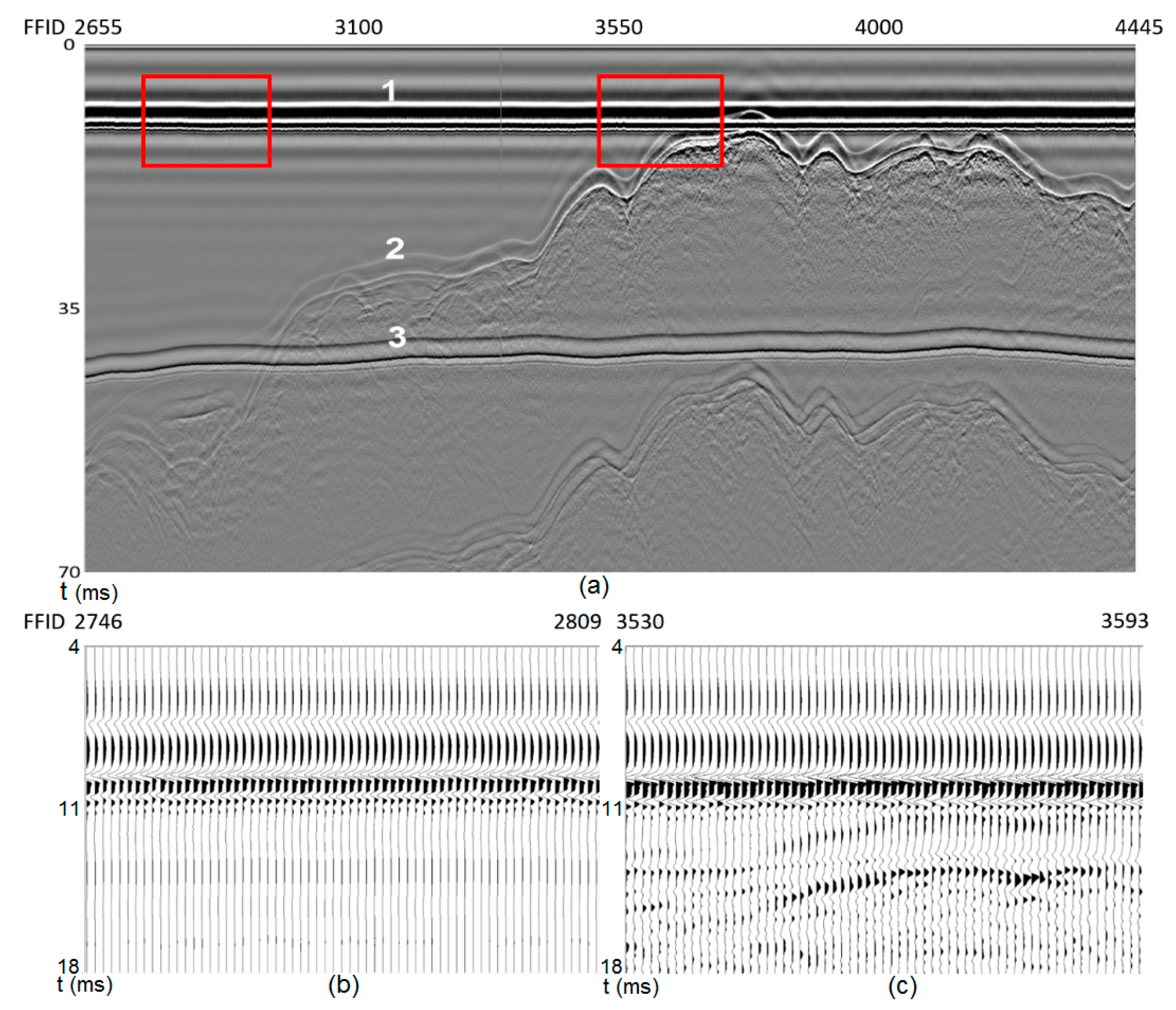
Figure 1a shows a part of the wavefield registered in one of the sections of the profile. It corresponds to the seismogram of equal offsets of the fifth spread channel. When obtaining it, band-pass filtering with parameters: Passband edge frequencies are 350 Hz and 3500 Hz, and stopband edge frequencies are 250 Hz and 4500 Hz, as well as correction for geometric front divergence was used. The specified frequency band was taken into account in the spectral analysis of the presented data.

It can be seen that on a significant part of the research profile, it is possible to accurately identify signals registered on small times and related to different types of waves. In this case, the signals of the direct wave are well separated from the signals of other waves, which makes it possible to study their features in detail, in particular, in the frequency domain. When calculating the spectra of direct wave signals, the interval duration was 6 ms. The start of the intervals was taken constantly with a small indent from the time arrival of the signal (see Figure 2).

We will not dwell on a detailed analysis of changes in the waveform and the amplitudes of its peaks. Such an analysis was performed in [13]. Note that even the signals presented in Figure 1b,c show some variations in the waveform, indicating possible changes in high-frequency components. Figure 1a also shows the change in the arrival time of the ghost reflection from the sea surface. Taking into account that the distance between the source and the receiver remained constant (as indicated by the invariability of the arrival times of the direct wave), such a change is probably associated with a change in the depth of the receiving-emitting system. As is known, the characteristics of the “Sparker” source depend, among other things, on the immersion depth of the source. Therefore, additional changes in the initial wavelet form may appear. However, such changes, most likely, will not be accidental, but natural.

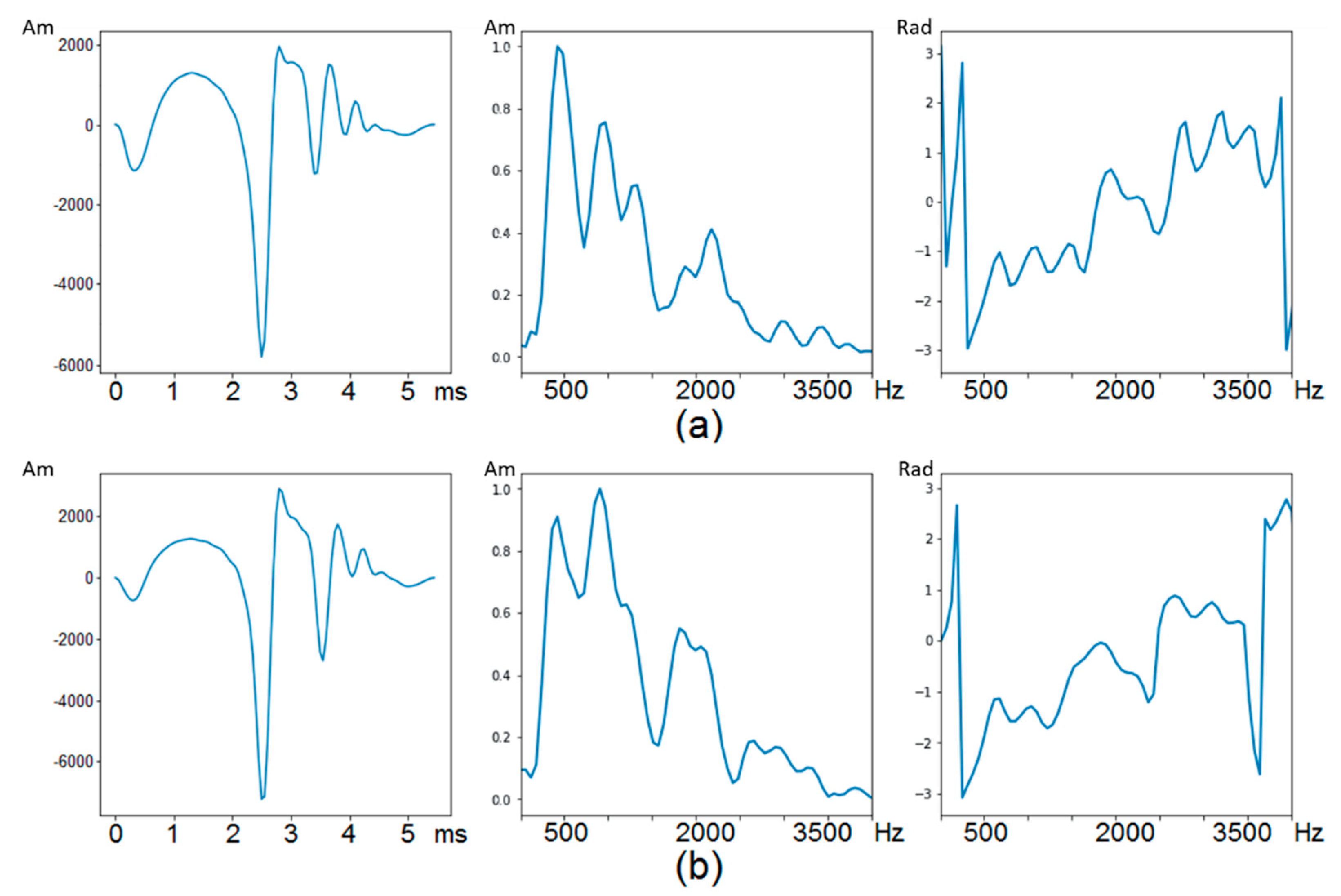
Figure 2 shows the analyzed signals of the direct wave and their spectra. The signals were taken from two different parts of the profile. It can be seen that they have insignificant variations (compare the left parts of Figure 2a,b). However, such changes lead to a significant difference in the spectral characteristics of signals when they are studied in a wide frequency range.

Small changes in a form of the direct wave, which can be considered the initial pulse (or wavelet) propagating in the medium under study, allows one to construct on their basis a deterministic deconvolution operator. Such an operator was calculated separately for each trace using the corresponding signal of the direct wave recorded on the same trace. As a result, a high resolution was achieved for the observed wave field, which made it possible to improve the quality of determining the structural elements of the medium [8]. It was assumed that as a result of the performed deconvolution, the variability of the initial impulse would also be fully eliminating. However, as will be shown below, this was not a completely correct assumption, and the remaining changes in the spectral characteristics of the direct wave signals can be significant.

2.2. Spectral Analysis of Target Signals

Signals of the direct wave obtained in the deconvolution process are shown in Figure 3a. Here is presented the corresponding part of each three hundredth traces. It can be seen that the signals are significantly compressed and have a simpler form. At the same time, there are residual variations in them, which can lead to essential variations in the frequency domain. To analyze such variations, we performed calculations of the spectra of compressed direct wave signals. In this case, a narrower interval was used than in the analysis of the initial signals. Its duration was 2.7 ms.

For clarity of the available variations in the wavefield, three traces with different waveforms are highlighted in red (Figure 3a). The observed changes in the analysis of the arrival times of signals appear to be insignificant and easily eliminated using the simplest correlation and summation procedures. However, the transition to spectral characteristics shows that they can significantly change the structure of the spectrum, especially when analyzing the phase component (see the right column of Figure 3b). This is due to the appearance of additional high-frequency components. In some cases, these components can be comparable in amplitude and energy to the main signal component. Therefore, for some of problems, for example, those related to the analysis of the finest-structured features of reflecting horizons or the determination of the characteristics of thin-layered deposits containing low-contrast internal reflections, such changes can lead to significant errors. They can also significantly affect the discrepancy between the observed waveform and theoretical constructions, implemented in the kind of numerical solutions to direct problems describing the interaction of seismic waves with bottom sediments.

In connection with the tasks of studying the interactions of seismic waves with bottom sediments, we will make one more remark related to the calculation of the spectra values of the analyzed signals. When performing such calculations, we need to ensure that the following three conditions are met:

(1)

The signals have a very short duration (a few milliseconds),

(2)

it is required to calculate with high accuracy the spectra values in a wide frequency band (from tens to thousands of hertz),

(3)

at calculating spectra for modeling or solving inverse problems may require a small step on frequencies (less than 1 hertz).

These conditions are difficult to fulfill using standard methods for calculating spectra. In our opinion, for these purposes, it is better to use special procedures focused on the high accuracy of calculating values of Fourier integrals with rapidly oscillating functions.

One of such procedures was implemented by us based on Filon’s method [15] with local parabolic interpolation of signal values. In addition to improving the accuracy of spectrum values calculating, such procedures have another advantage. It consists in the fact that we can calculate the spectrum value for any frequency values. Thus, we have no restrictions on the step between frequencies.

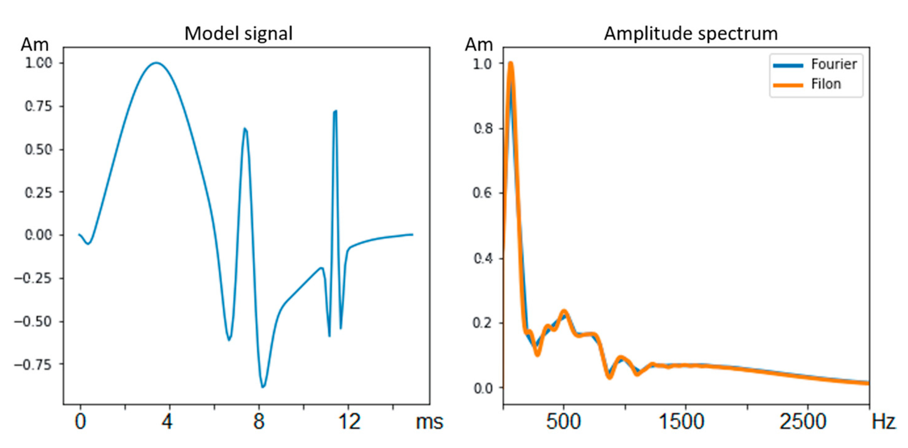
Figure 4 shows a modeled example that illustrates how the created procedure works. The modeled signal was formed based on three Riker impulses with frequencies: 80 Hz, 500 Hz, and 1500 Hz, with different time delays from the beginning of the analysis interval. The kind of signal is shown on the left side of Figure 4. The right side of this figure shows a comparison of the spectrum values calculated by the two types of procedures. It can be seen that even for a fairly simple signal, Filon’s method provides a spectrum with greater detail of its features.

2.3. Factor Decomposition in the Spectral Domain

Analysis of changes in the calculated spectra at a fixed frequency can be performed based on histograms. This will make it possible to define the structure of the variations. However, it will not allow us to better understand their nature, which can be very complex. For a deeper study of the existing changes, we used factor models (Appendix A). They make it possible to assess the influence of multiplicative components on the seismic signal form [16]. Such components can describe a change in the signal associated both with the conditions of the experiment and with interactions with the medium. The former are unwanted factors that require elimination, while the latter can be used to study the effects of the interaction of seismic waves with bottom sediments.

Selecting signals of direct wave simplifies the research task. In this case, there is no interaction of signals with the target medium. Therefore, it is possible to use fairly simple factor models. We used one of the simplest factor models, which has the following form:

$$z_{ij}\left(\omega \right)={\alpha }_i\left(\omega \right)+{\beta }_j\left(\omega \right)+{\epsilon }_{ij}\left(\omega \right)$$

(1)

Here, $z_{ij}\left(\omega \right)$ are the logarithms of the amplitude spectra of the analyzed signals, i.e., $z_{ij}\left(\omega \right)=\ln \left\{\left|S_{ij}\left(\omega \right)\right|\right\},$ and $\omega =2\pi f,$ where $f$ is the frequency measured in hertz. Indexes $i,j$ define the position of sources and receivers in the system of observations. Therefore, the components: ${\alpha }_i\left(\omega \right),$ ${\beta }_j\left(\omega \right)$ can determine possible changes in signal spectra associated with changes in the characteristics of sources and receivers, and the component ${\epsilon }_{ij}\left(\omega \right)$ will include all remaining changes in the spectra.

At a fixed frequency, model (1) takes the simplest form:

$$z_{ij}={\alpha }_i+{\beta }_j+{\epsilon }_{ij}$$

(2)

In this case, the remaining changes ${\epsilon }_{ij}$ will not depend on the frequency, and we can represent them in the form of a histogram of values ${\epsilon }_{ij}$=$z_{ij}-{\tilde{\alpha }}_i-{\tilde{\beta }}_j$. To do this, we just need to determine the values of estimates of the factors:${\tilde{\alpha }}_i, {\tilde{\beta }}_j$. Based on the obtained estimates of the factors for all analyzed frequencies, the corrected values of the spectra of the target signal can be determined as

$${\tilde{z}}_{ij}\left(\omega \right)=z_{ij}\left(\omega \right)-{\tilde{\alpha }}_i\left(\omega \right)-{\tilde{\beta }}_j\left(\omega \right)$$

(3)

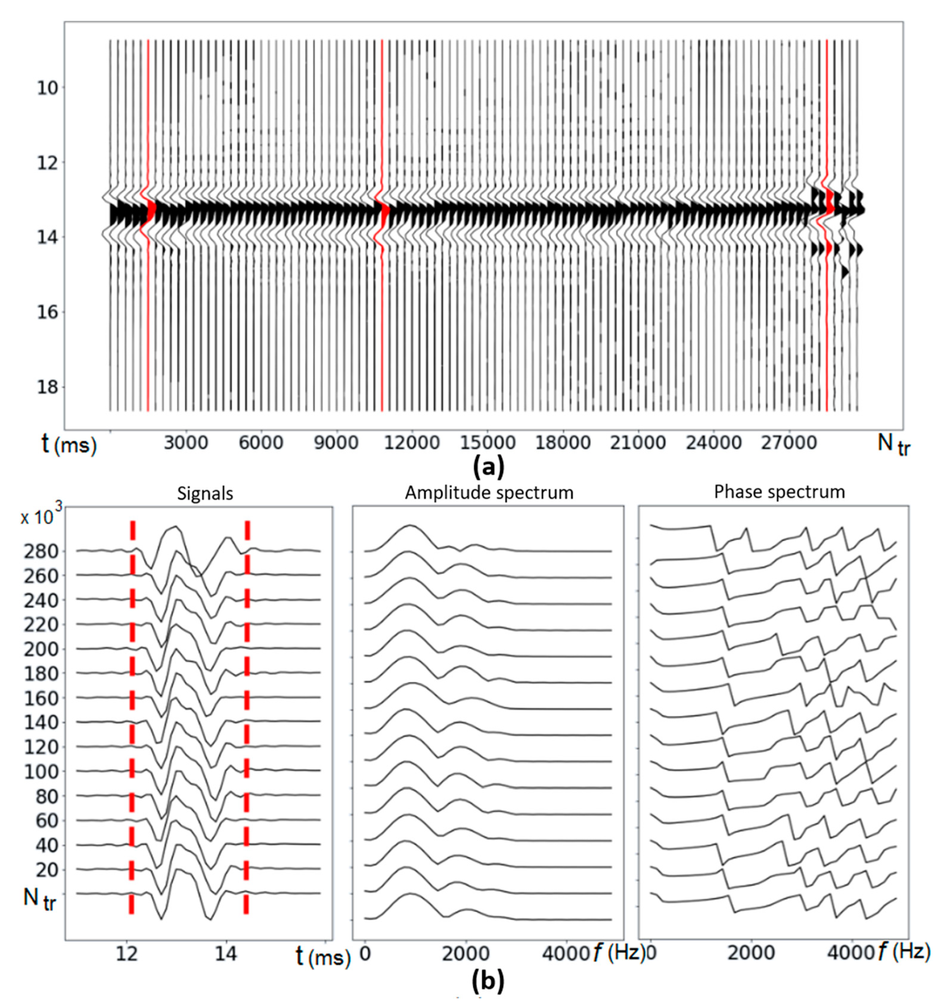
When determining the indicated values of estimates of the factors, we faced one interesting problem. The fact is that when determining the direct wave signals, we had to skip the areas where there was interference with reflections from the bottom sediments. Thus, the structure of the observing system became irregular. Therefore, we decided to use a simple iterative factor estimation method. Its idea is very simple. First, we estimate the first factor ${\alpha }_i$, assuming that the second factor is absent. Then we subtract those obtained from the initial values $z_{ij}$ and proceed to assess the values of the second factor ${\beta }_j.$ Having received the estimates of the second factor, we subtract their initial values $z_{ij}$ and return to the estimation of the values of the first factor. The software implementation of the procedure, which can be called the process of consistent refinement of parameter estimates, is very simple and, as it seemed to us, does not depend on the structure of the system of observations.

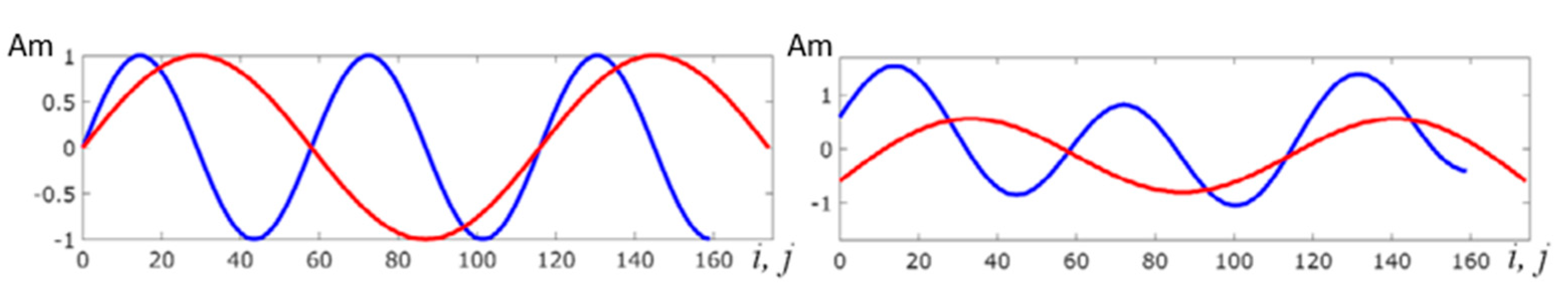
But when we started testing it, we found an interesting effect. At first, we perceived it as a software error. This effect is illustrated in Figure 5. On the left, the colors show the values of the factors: Blues are values of ${\alpha }_i$, and reds are values of ${\beta }_j$. These values were used to form model values $z_{ij}={\alpha }_i+{\beta }_j$, which were then fed to the input of the iterative process to determine them. The estimates of factors obtained as a result of 10 refining iterations are shown in the right part of the figure. It can be seen that they differ significantly from the initial values. At the same time, an increase in the number of iterations did not lead to an improvement in the obtained values of the factors.

The main difficulties for our understanding of this result were as follows. First, we knew that the iterative process of consistent refinement of parameter estimates is convergent. In this case, he must converge to the solution of the system of equations of the method of least squares (MLS). Second, for the system of equations MLS, which corresponds to model (2), there is non-uniqueness in relation to the definition of a constant value included in each of the factors. However, we have observed complex changes in the estimates obtained, which indicated a redistribution of long-period components between the values of the factors. This effect is known as the long-period statics problem. To find out the reasons for the appearance of this effect when working with the presented data, we are carrying out a separate large study. Its results will be published in a special article.

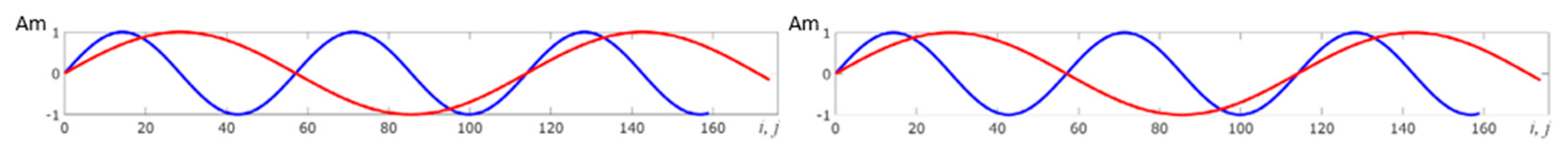
As a result, we had to abandon the use of a simple iterative method and apply a more complex matrix method described in [17]. It made it possible to obtain accurate estimates of the factors in the model experiment, which differed from the true ones by a small constant value. The corresponding result is shown in Figure 6. Therefore, in the future, this method was used to analyze the spectra.

3. Results and Discussion

As mentioned in the previous section, histograms are the main ones used in analyzing changes. They allow a better determination of the structure of variations than individual characteristics, in particular, the standard deviation, which provides a complete definition only in the case of a normal distribution. However, as will be shown below, the distributions differ significantly from the normal and often have non-unimodality. When constructing histograms, two types of quantities were used: The values of the amplitude spectra of direct wave signals at a fixed frequency, normalized to the average value of the spectrum, and the logarithms of these values. We needed the second type of quantities when using factor models (1)–(2) that provide a partial account of the existing changes in the spectra.

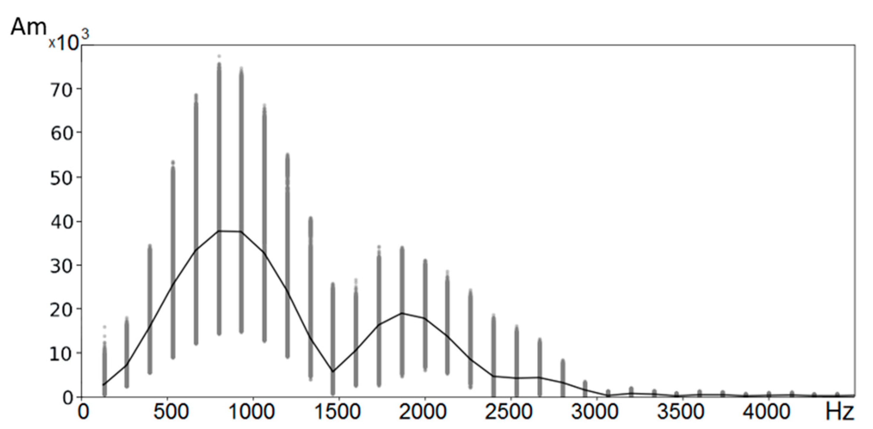
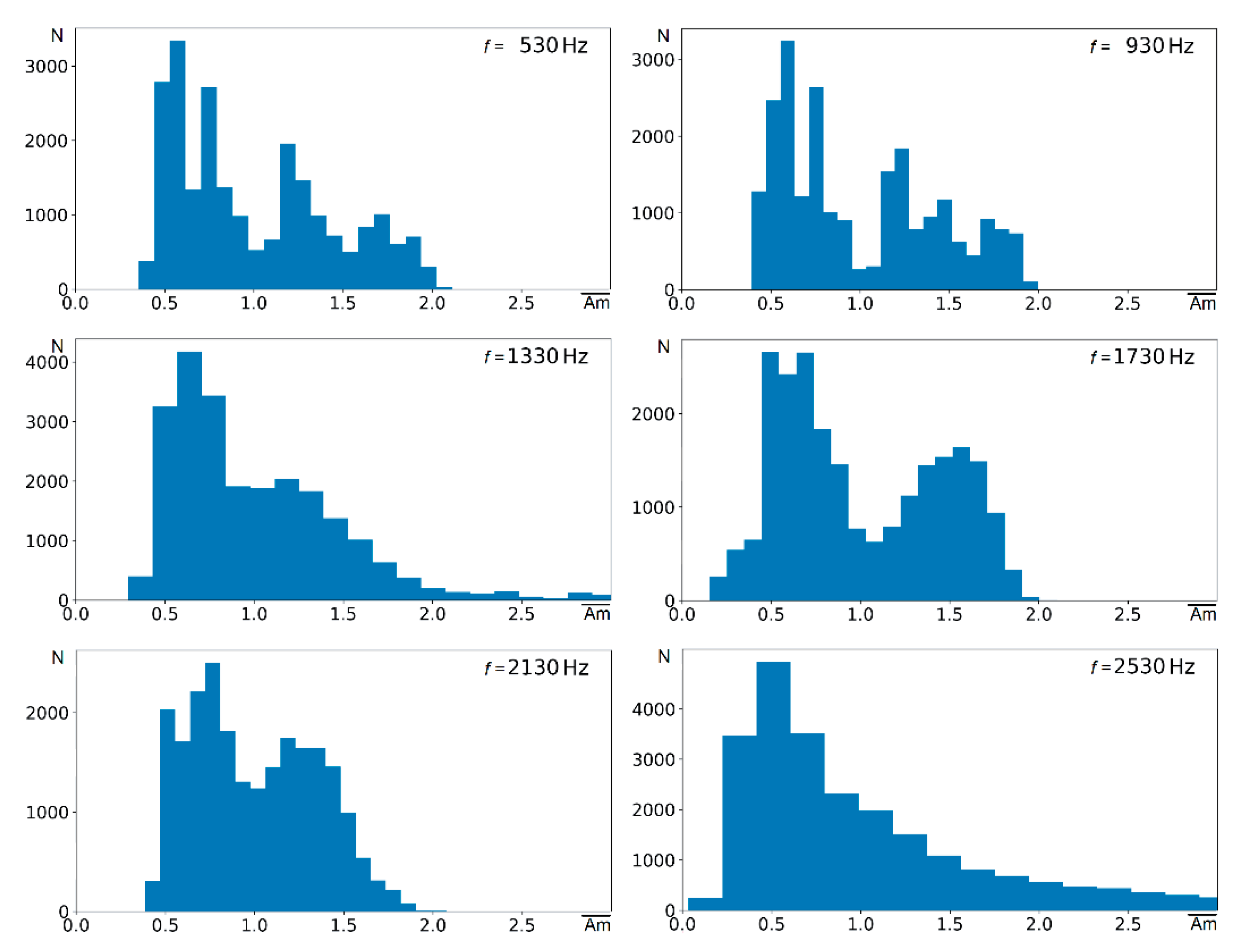
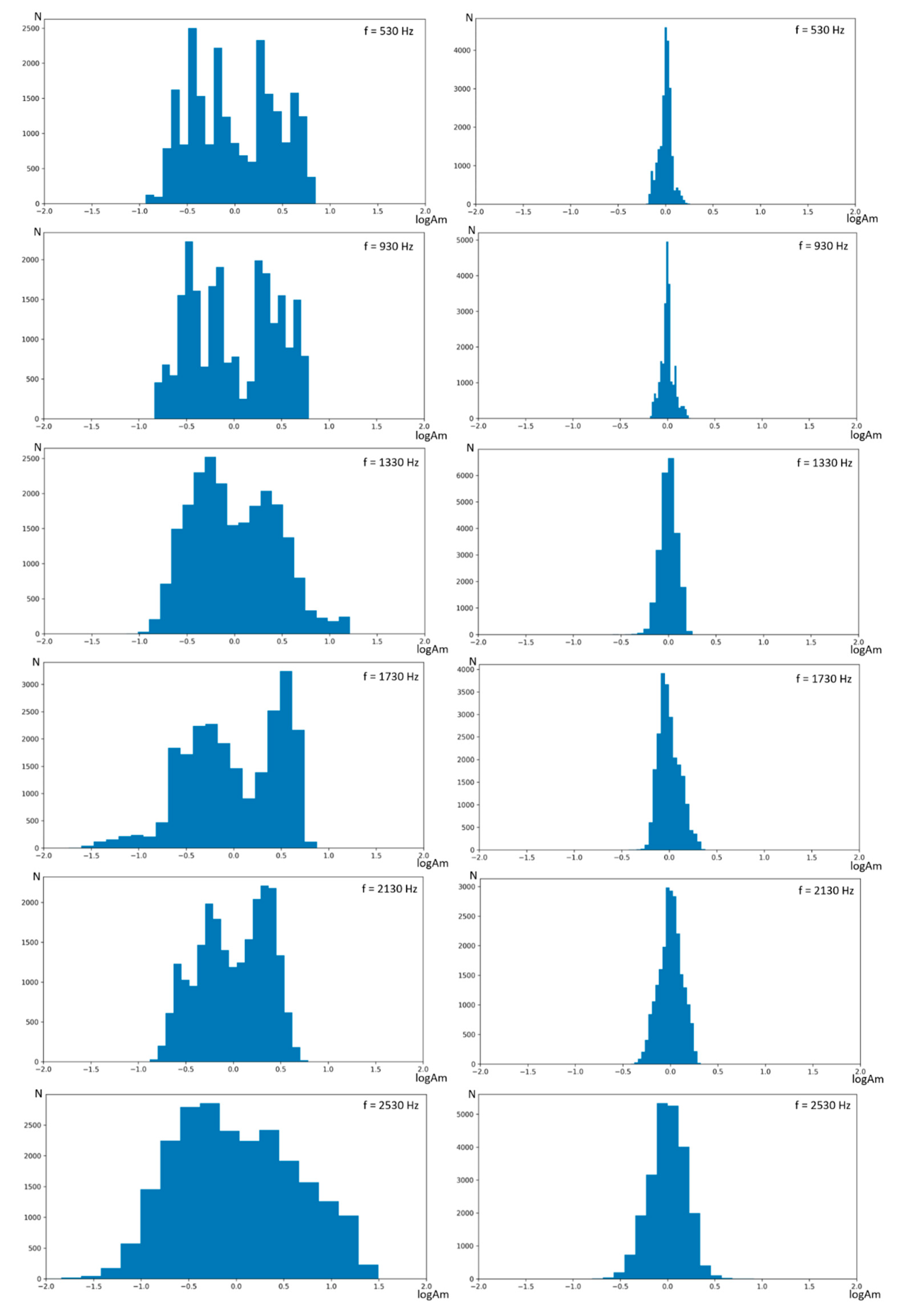
Figure 7 shows in gray the spectral values calculated at fixed frequencies for all analyzed signals of the direct wave. The total number of signals exceeded 30,000. The black line shows the values of the average spectrum. Even visual assessment indicates significant variations in the spectral characteristics of the signals. For a better understanding of the structure of the available variations, Figure 8 shows histograms plotted using the values of the normalized spectra at frequencies: 530 Hz, 930 Hz, 1330 Hz, 1730 Hz, 2130 Hz, and 2530 Hz. The selected frequencies belonged to different bands, so the histograms give an idea of the changes in the spectra in the entire analyzed frequency domain.

The histograms show a substantially non-unimodal and asymmetric nature of changes in the values of the spectra. The normalized values of the spectra make it possible to assert that the changes can reach 100%, and sometimes even exceed them. Such situations are especially typical for high frequencies. The complex structure of the distributions of spectral variations can lead to two important points. The first is associated with the construction of procedures for the rejection of signals with significant variations in the spectral composition. Especially, this moment becomes significant when analyzing complex reflections from bottom sediments. The second point concerns the creation of criteria for testing hypotheses about the correspondence of the proposed mathematical models of the interactions of seismic waves with bottom sediments to real processes. In the case of complex and non-stationary distributions, such criteria are almost never constructed, and when trying to construct them, very unreliable results are obtained.

The use of the model (2) with the estimation of the factors of sources and receivers in the log-spectral region made it possible to obtain a significant decrease in variations in the entire analyzed frequency range. Figure 9 shows the histograms of the values of the logarithms of the spectra for the same frequencies: 530 Hz, 930 Hz, 1330 Hz, 1730 Hz, 2130 Hz, and 2530 Hz, which were used to construct the histograms of Figure 8. The left column contains histograms of the initial values, and the right column of histograms are plotted by residual values. It can be seen that the residual changes in the spectra after the elimination of the changes associated with the sources and receivers became significantly smaller. However, the most important point is that the structure of histograms has improved. They became unimodal and approached a normal distribution.

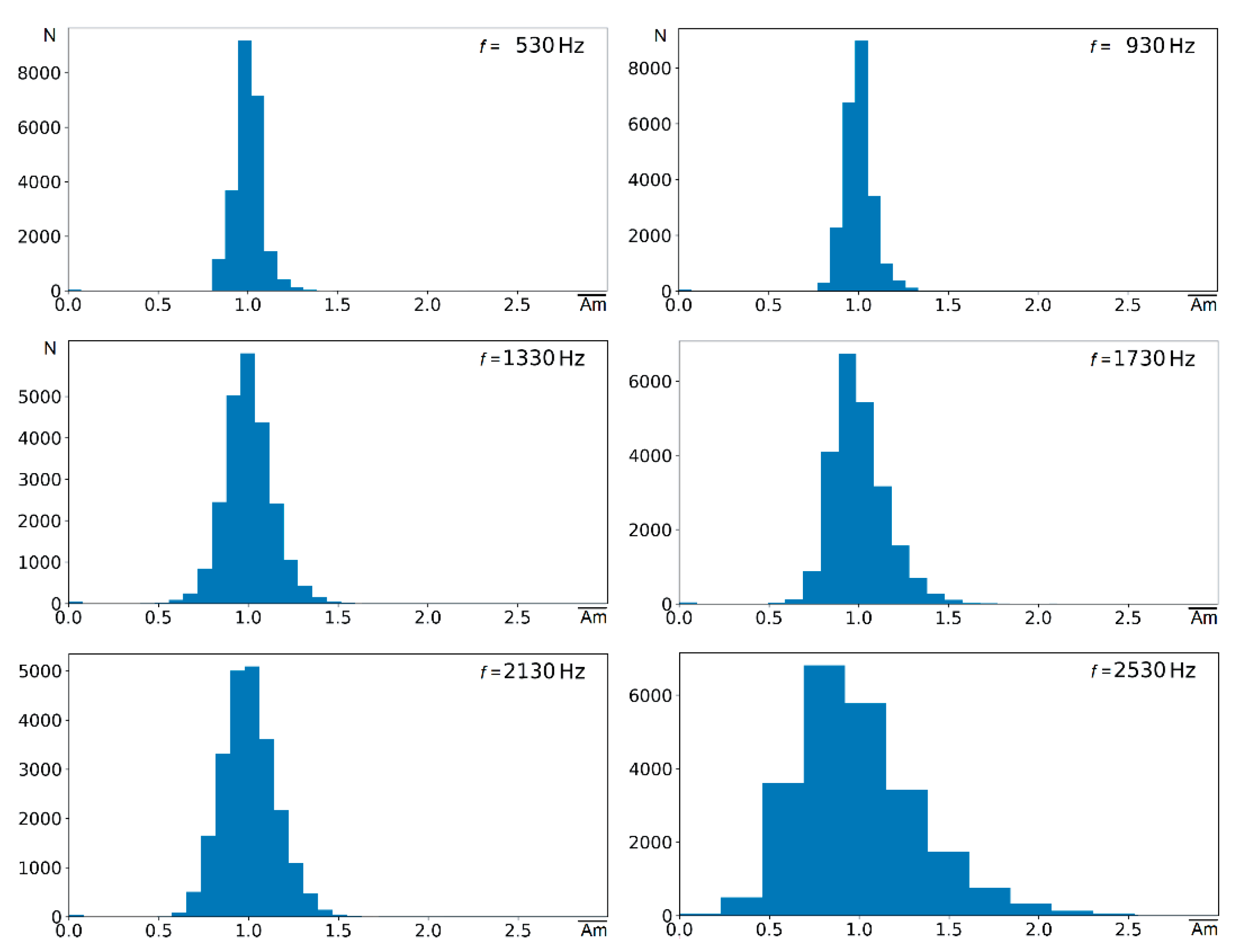
Figure 10 shows the values of the amplitude spectra of direct wave signals, corrected using the obtained estimates of factors for sources and receivers, according to (3). It is seen that compared to the original spectra shown in Figure 7, the corrected spectra have significantly smaller variations in the frequency band up to 2500 Hz. However, for a more detailed description of the variations, let us look at the histograms of the values of the corrected spectra, which are presented in Figure 11.

Analysis of the histograms which are given in Figure 11 indicates a significant improvement in the structure of the distributions of the spectra values after the made-up correction. It is seen that their changes for a wide frequency band do not exceed 50%. Moreover, the use of simple rejection procedures will help reduce the variability of the spectra to 20–30%. An essential point is the question of the variability of the spectra in the high-frequency region, exceeding 2500 Hz. As follows from the histogram obtained at a frequency of 2530 Hz, there is an asymmetry and a wide swing of the residual additive component here.

Our approach improves the quality of real data that determines the results of seismic processing (migration transformations, deconvolution, and AVO). In turn, the processing results increase the accuracy in studying the interactions of seismic waves with bottom sediments.

The limitations of the method are related to the type of the factor model and its correspond to real data. Based on factor decomposition, we can correct the reflected waveform.

4. Conclusions

The results obtained allow us to draw the following conclusions:

• Research has shown that there is significant variability in the data. Therefore, it is required to develop methods for taking into account the existing changes, in particular, those related to the characteristics of excitation and reception of oscillations in a wide frequency range.
• Using the method of factor decomposition in the spectral domain significantly reduces the changes associated with the sources and receivers, which could improve the data quality of marine surveys from hundreds of hertz to kilohertz.
• In the course of the research, the problem of determining long-period components was discovered when using the iterative process.
• Development is required for seismic signal correction methods in a wide range of seismic frequencies.
• Studying the interaction of waves with bottom sediments may be changed in the characteristics of reflection from the angle of incidence of the wave on the target object. Such information may turn out to be extremely important, but to obtain it, it is necessary to use more complex factor models for representing the wavefield during processing [16].

References

- Bjersted, D. NMO distortion. Can. J. Explor. Geophys. 1995, 3, 25–31. [Google Scholar]
- Jafar Gandomi, A.; Hoeber, H.; Lacombe, C.; Souvannavong, V. Effective Delivery of Reservoir Compliant Seismic Data Processing. In Proceedings of the AAPG/SEG 2017 International Conference and Exhibition, London, UK, 15–18 October 2017. [Google Scholar]
- Szymańska-Małysa, Z.; Dubiel, P. 3C seismic data processing and interpretation: A case study from Carpathian Foredeep basin. Acta Geophys. 2019, 67, 2031–2047. [Google Scholar] [CrossRef] [Green Version]
- Alcalde, J.; Bond, C.; Johnson, G.; Kloppenburg, A.; Ferrer, O.; Bell, R.; Ayarza, P. Fault interpretation in seismic reflection data: An experiment analyzing the impact of conceptual model anchoring and vertical exaggeration. Solid Earth 2019, 10, 1651–1662. [Google Scholar] [CrossRef] [Green Version]
- Hutapea, F.; Tsuji, T.; Katou, M.; Asakawa, E. Data processing and interpretation schemes for a deep-towed high-frequency seismic system for gas and hydrate exploration. J. Nat. Gas Sci. Eng. 2020, 83, 103573. [Google Scholar] [CrossRef]
- Cichostepski, K.; Dec, J.; Kwietniak, A. Simultaneous Inversion of Shallow Seismic Data for Imaging of Sulfurized Carbonates. Minerals 2019, 9, 203. [Google Scholar] [CrossRef] [Green Version]
- Henrique do Prado, A.; Paes de Almeida, R.; Tamura, L.; Galeazzi, C.; Ianniruberto, M. Interpretation software applied to the evaluation of shallow seismic data processing routines in fluvial deposits. Braz. J. Geol. 2019, 49, 579–594. [Google Scholar]
- Pirogova, A.; Tikhotskii, S.; Tokarev, M.; Suchkova, A. Estimation of Elastic Stress-Related Properties of Bottom Sediments via the Inversion of Very- and Ultra-High-Resolution Seismic Data. Izv. Atmos. Ocean. Phys. 2019, 55, 1755–1765. [Google Scholar] [CrossRef]
- Dondurur, D. Acquisition and Processing of Marine Seismic Data; Elsevier: Amsterdam, The Netherlands, 2018. [Google Scholar]
- Tokarev, M.; Kuzub, N.; Pevzner, R.; Kalmykov, D.; Bouriak, S. High resolution 2D deep-towed seismic system for shallow water investigation. First Break 2008, 26, 77–85. [Google Scholar] [CrossRef]
- Madatov, A.; Mitrofanov, G.; Sereda, V. Approximation approach in dynamic analysis of multichannel seismograms. 3. Application aspects. Geol. Geophys. (Soviet) 1992, 33, 4. [Google Scholar]
- Mitrofanov, G.; Helle, H.; Kovaliev, V.; Madatov, A. Complex seismic decomposition—Theoretical aspects/Extended Abstracts of papers. In Proceedings of the EAEG 55th meeting, Stavanger, Norway, 7–11 June 1993. [Google Scholar]
- Goreyavchev, N.; Isayenkov, R.; Mitrofanov, G.; Tokarev, M. Variability of wavelet form in seismic marine in marine investigations. Seism. Technol. 2016, 4, 67–76. [Google Scholar]
- Yilmaz, O.; Baysal, E. An Effective Ghost Removal Method for Marine Broadband Seismic Data Processing. In Proceedings of the IFEMA Madrid, Madrid, Spain, 1–4 June 2015. [Google Scholar] [CrossRef] [Green Version]
- Filon, L.N.G. On a quadrature formula trigonometric integrals. Proc. R. Soc. Edinb. 1928, 49, 38–47. [Google Scholar] [CrossRef]
- Mitrofanov, G. Effective presentation of the wave field in seismic exploration. Geol. Geophys. (Soviet) 1980, 21, 46–58. [Google Scholar]
- Mitrofanov, G.; Rachkovskaia, N. A priori information forming for analyzing and correction of seismic data in reflection waves method. Geol. Geophys. (Soviet) 1996, 37, 93–102. [Google Scholar]
Figure 1.
Examples of the wavefield registered on the investigated profile: (a) For an extended section of the profile and a time interval of 70 ms; (b) for the middle part of the profile in the direct wave region; (c) for the right-hand part of the profile, where the interference of the direct wave with reflections from the bottom sediments is observed. The numbers in figure (a) indicate the types of waves: 1—direct wave, 2—reflected wave from the seabed, 3—the ghost reflection from the sea surface. The red frames in figure (a) denote the direct wave interval. The left frame is the signal of the direct wave without interference—figure (b). The right frame is a direct wave signal with interference—figure (c).
Figure 2.
From left to right: The signal form of the direct wave, amplitude spectrum values, phase spectrum values. (a) Middle of the profile (signal from the left red frame at Figure 1a), (b) near the region of interference with reflections from bottom sediments (signal from the right red frame at Figure 1b).
Figure 3.
Analysis of signals of the direct wave after deconvolution. (a) A part of the wavefield. (b) From left to right: Analyzed signals and their amplitude and phase spectra. Red markers show a narrow time interval for calculating spectra.
Figure 4.
Calculation of the spectrum from the model signal using the standard procedure and based on Filon’s method. The blue color on the right side of the figure displays the Fourier transform result and the orange color on the right side of the figure displays the Filon transform result.
Figure 5.
A model experiment to separate factors using the iterative process of consistent refinement of parameter estimates. The red color shows the receiver factor and the blue color shows the source factor.
Figure 6.
Model experiment on separation of factors using the matrix estimation method. The red color shows the receiver factor and the blue color shows the source factor.
Figure 7.
The values of the spectra of the analyzed signals.
Figure 8.
Histograms of the original spectra are plotted for six frequencies (the frequency values are given in the figures).
Figure 9.
Histograms are plotted in the log-spectral region for six frequencies (frequency values are given in the figures, and explanations in the text). The left column shows histograms of spectra before factor decomposition. The right column shows histograms of spectra after factor decomposition.
Figure 10.
The values of the corrected spectra of the signals.
Figure 11.
Histograms of corrected spectra are plotted for six frequencies (the frequency values are given in the figures).
Publisher’s Note: MDPI stays neutral with regard to jurisdictional claims in published maps and institutional affiliations. |
© 2021 by the authors. Licensee MDPI, Basel, Switzerland. This article is an open access article distributed under the terms and conditions of the Creative Commons Attribution (CC BY) license (http://creativecommons.org/licenses/by/4.0/).
Share and Cite
MDPI and ACS Style
Mitrofanov, G.; Goreyavchev, N.; Kushnarev, R. Improving Accuracy in Studying the Interactions of Seismic Waves with Bottom Sediments. J. Mar. Sci. Eng. 2021, 9, 229. https://0-doi-org.brum.beds.ac.uk/10.3390/jmse9020229
AMA Style
Mitrofanov G, Goreyavchev N, Kushnarev R. Improving Accuracy in Studying the Interactions of Seismic Waves with Bottom Sediments. Journal of Marine Science and Engineering. 2021; 9(2):229. https://0-doi-org.brum.beds.ac.uk/10.3390/jmse9020229
Chicago/Turabian StyleMitrofanov, Georgy, Nikita Goreyavchev, and Roman Kushnarev. 2021. "Improving Accuracy in Studying the Interactions of Seismic Waves with Bottom Sediments" Journal of Marine Science and Engineering 9, no. 2: 229. https://0-doi-org.brum.beds.ac.uk/10.3390/jmse9020229
Note that from the first issue of 2016, this journal uses article numbers instead of page numbers. See further details here.