Article

Virtual Level Analysis Applied to Wave Flume Experiments: The Case of Waves-Cubipod Homogeneous Low-Crested Structure Interaction

by
Mireille Escudero
1,
Jassiel V. Hernández-Fontes
2,
Irving D. Hernández
3 and
Edgar Mendoza
1,*
1
Instituto de Ingeniería, Universidad Nacional Autónoma de México (UNAM), Edificio 17, Ciudad Universitaria, 04510 Mexico City, Mexico
2
Departamento de Engenharia Naval, Escola Superior de Tecnologia, Universidade do Estado do Amazonas (UEA), Av. Darcy Vargas 1200, Parque Dez de Novembro, 69050-020 Manaus, Brazil
3
Núcleo de Estruturas Oceânicas—NEO, Programa de Engenharia Oceânica, COPPE, Universidade Federal do Rio de Janeiro, Centro de Tecnologia, Bloco I-208, Cidade Universitária, 20945-970 Rio de Janeiro, Brazil
*
Author to whom correspondence should be addressed.
J. Mar. Sci. Eng. 2021, 9(2), 230; https://0-doi-org.brum.beds.ac.uk/10.3390/jmse9020230
Submission received: 24 December 2020 / Revised: 21 January 2021 / Accepted: 8 February 2021 / Published: 22 February 2021
(This article belongs to the Special Issue Breakwater Behaviour)

Abstract

:
This paper presents the use of virtual level (VL) probes as an alternative image-based approach to investigate the interaction of waves with coastal structures in wave flume experiments. These probes are defined as regions of interest located at specific positions along the horizontal domain of the images, in which edge interfaces are detected and, thus, their vertical motions can be obtained. To demonstrate the use of the methodology, a critical condition of breaking waves interacting with a Cubipod homogeneous low-crested structure (HLCS) in a two-dimensional framework was selected. With the video recorded from the experiments, image calibration, processing, and analysis stages were implemented to analyze the performance of the HLCS in reducing wave elevations and to study the stability of the armor units. The present approach can be extended to a wide range of coastal structures applications where the interface detection between components of the scene is useful to observe the behavior of coastal structures, increasing effectiveness and alternatives to acquire precise data in 2D experimental tests.

1. Introduction

Laboratory wave flume experimentation is a widely used practice by scientists and engineers to understand the physical processes taking place in coastal environments. The spatial and the temporal variations of the water surface elevation are essential data observed in this field that remain mostly measured with traditional capacitance, conductive, and resistance wave gauges. As an example of application, small-scale tests of damage monitoring in rubble mound breakwaters have been addressed for more than 80 years, and continuous advances in the applied measurement methods have been proposed to evaluate the stability of breakwaters [1]. Recent studies have shown the extensive applicability of image processing tools in multiple fields of research and their growing adaptation to studies in coastal and ocean research [2,3,4].
Being costly, intrusive, spatially constrained, and inaccurate readings affected by entrapped air in the fluid are some of the disadvantages identified from the use of traditional wave probes to measure the water elevation in small-scale experiments [2,4]. Viriyakijja and Chinnarasri [4] presented the application of CCD video cameras with edge detection algorithms to measure the water surface elevation in the laboratory as an innovative, easy, low-cost, and accurate alternative method to the use of wave gauges. Recently, Douglas et al. [2] described an image-based method for the automatic detection of water surface using color segmentation. The image processing method was further extended to compute wave run-up characteristics and dynamic loads acting on the armor units of rubble mound breakwaters.
Despite the measurements of water surface, image-based approaches are also useful to study motion of structural members. Classical methods for quantitative measurements of armor damage are mainly based on counting the number of dislodged armor units by means of a fixed camera (visual counting), accomplished by photo overlays or flickering technique (counting process) or expressed as the eroded area/volume in relation to a non-damaged section after the application of a laser profiler to reconstruct the 2D/3D cross-section of the breakwater [1]. Difficulties for the application of these methods have been identified for high levels of damage [5,6].
Visual counting was only recommended for low and moderate damage levels, only if porosity of the armor layer was constant [5]. The virtual net method was presented to take into account the heterogeneous packing failure mode due to the variation in porosity in different parts of the breakwater, which enables the counting of the number of armor units in each of the strips resulting from the projection of a virtual net over the armor layer photograph [7,8]. However, as mentioned by [9], the application of each of these traditional techniques is limited to specific conditions and damage levels. Some disadvantages of the use of mechanical profilers have been also presented, such as the intrusive nature of the instrument that could affect the measurement precision by possible induced movements of armor units, the lack of a standardized method specifying the optimal accuracy or the required number of profiles, and the systematic error given by the accuracy of the positioning of the device and the accuracy of the measurements [1,6].
The technological development in post-processing and graphic tools has encouraged the use of non-intrusive instrumentation and new scanning instruments as substitutes of traditional tools and techniques, though evidence of their application in laboratory has not been found since 2003 [1]. Among these alternative methods are digital terrestrial photogrammetry and terrestrial laser scanner, infrared scanners, laser scanners, ultrasonic sensors, structure from motion (SfM) techniques, or digital stereo photography (DSP) [1,4]. An example is the application of laser scanning, stereo photogrammetry, and Kinect motion sensor to assess the armor layer damages on a rubble mound breakwater composed by rock and Antifer cubes, showing the good performance of these innovative survey techniques to evaluate eroded volumes in breakwaters [10].
Recently, alternative and simplified methods based on the concept of virtual water surface measurements at specific locations in wave flume experiments have been proposed for hydraulic applications [11] and ocean engineering research [12,13]. To the best of the authors’ knowledge, Kocaman and Ozmen-Cagatay [11] introduced the concept of virtual wave probe (VWP) measurements evaluating the flow from wet dam-break experiments. This definition was given to the water elevation measurements taken from videos in the wave flume tests. More recently, motivated by this concept, Hernández et al. [14] proposed a simplified image-based technique based on the VWP concept to measure water heights at specific locations over the horizontal domain. This approach is based on binary images, in which morphological operations are performed inside regions of interest (ROIs), located at desired locations along the horizontal image domain. This algorithm is open source and fast and was recently extended by [15] to measure multiple-valued water surfaces in some 2D hydrodynamic applications. The approaches based on defining regions of interest to perform the measurements (i.e., virtual sensors) can save computational time, since the measurements are taken only at the desired locations. If several virtual sensors are placed, then a 2D visualization of the object motion in time and x-direction space can be performed in a practical way.
As coastal structures research commonly occurs in wave flume experiments, the use of virtual sensors to track motion inside regions of interest could allow measurements of both water and structure motions in a 2D framework. This non-obstructive approach would allow capturing motion where it is difficult to place obstructive sensors, providing new relevant data for numerical model validation.
This paper presents an image-based study of the interaction of waves with a coastal structure in wave flume experiments using the concept of virtual level (VL) sensors. These sensors can be defined as ROIs set at specific positions in which the edge interfaces are detected, and their displacements are measured. The main objective is to verify the applicability of VL sensors to: (1) analyze the motion of the waves before and after interacting with the structure and (2) detect failure (displacement of armor units) at the crown of the structure in a 2D framework. To test the methodology, the case of breaking waves interacting with a Cubipod homogeneous low-crested structure (HLCS) [16] was considered. The selection of this type of structure was motivated by the fact that it is a novel alternative for artificial reef construction, which presents some advantages over conventional LCS [16,17,18].
The waves were designed to break just after interacting with the structure, resembling a critical design condition. Scene elements differentiation setup, background illumination techniques, and conventional video at 100 fps were employed for implementing the stages of image calibration, processing, and analysis. The contributions of the present work can be described as follows:
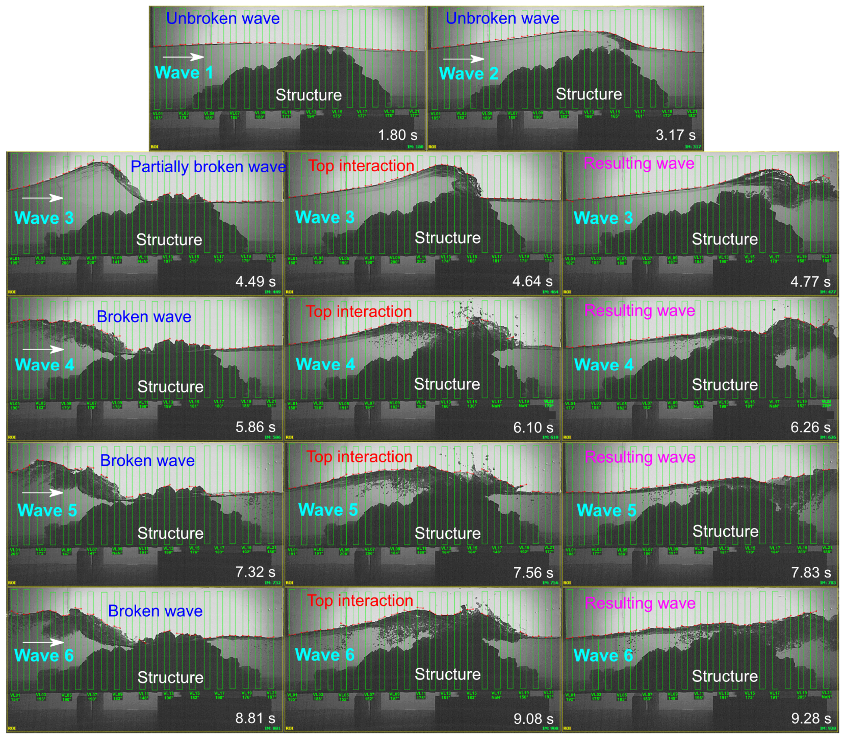
  • Details of the violent interaction of breaking waves with a Cubipod HLCS, which are critical conditions at which they can be subjected, were investigated.
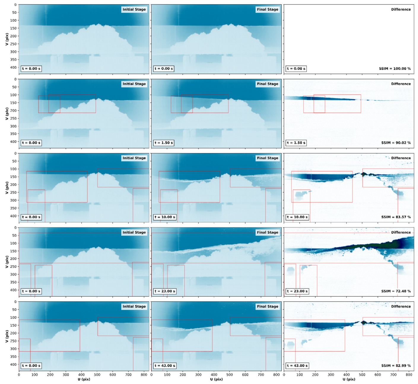
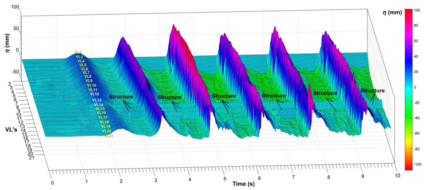
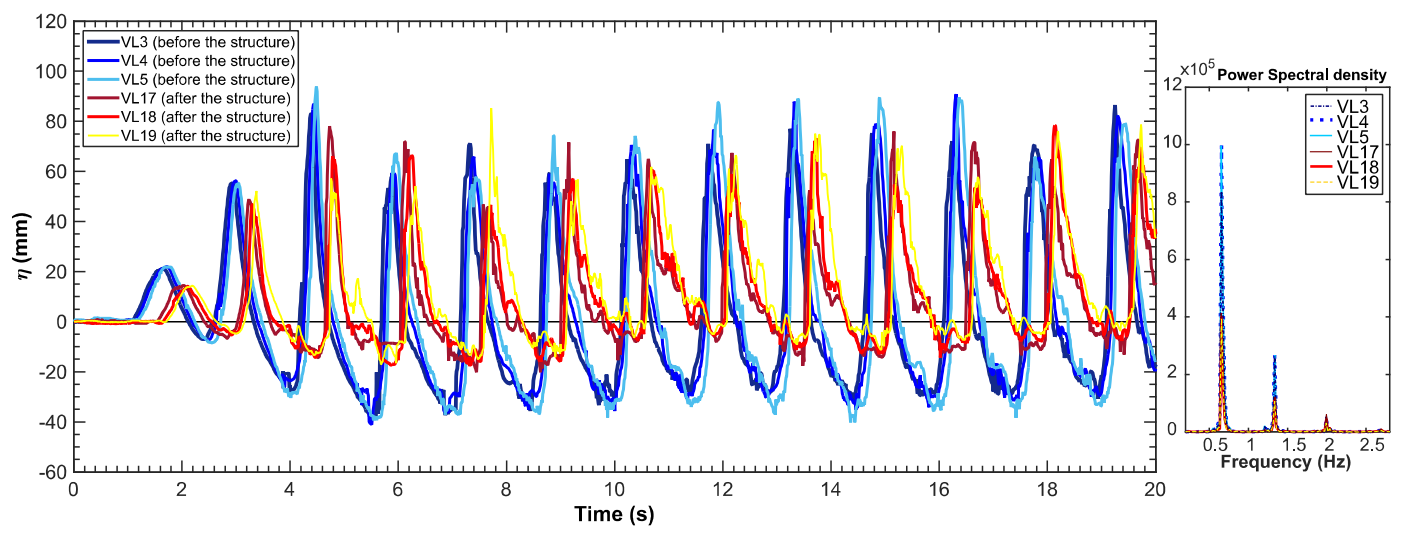
  • We investigated the spatio-temporal evolution of water elevations before and after interaction of the incident waves with the structure following a 2D assumption. This approach can provide useful data for detailed model validations in this type of research.
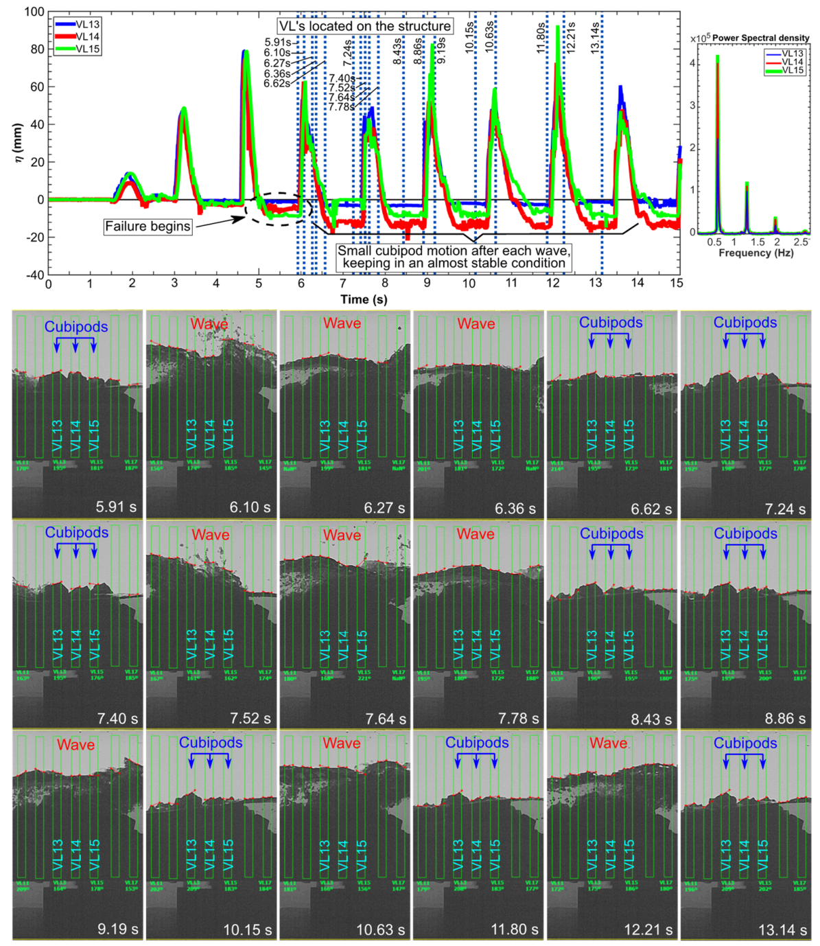
  • With the use of VL measurements, it was possible to track slight variations of Cubipods located above the water free surface, identifying the instants of failure of the top of the structure during the wave interactions.
The work is organized as follows: Section 2 presents the experimental setup, including the general arrangement, the procedure to install the structure, and the case of study. Section 3 shows the image-based approaches, including the stages of image calibration, processing, and analysis. Next, Section 4 presents results and discussion, providing qualitative and quantitative analyses of the wave–structure interactions. This section includes the spatio-temporal analysis of water elevations and the analysis of failure of the crest of the structure. Finally, Section 5 summarizes the main conclusions of this work.

2. Physical Tests

2.1. Experimental Set Up

The 2D experimental tests (scale 1/42.8) were performed in a wave flume (22.0 m× 0.4 m× 0.5 m) at Universidad Nacional Autónoma de México (UNAM) to study the interaction of breaking waves with a five-layer Cubipod HLCS (Figure 1a). Regular waves of 0.13 m height and 1.5 s period were generated with a piston type wavemaker (equipped with an active absorption system) located at the left side of the flume (see Figure 1b). It is worth mentioning that, although regular wave parameters were used to activate the wavemaker, the observed waves resembled a train of solitary waves caused by a fission process, which is a common phenomenon that occurs when cosine waves develop over shallow conditions [19,20]. At the downstream end of the flume, a passive absorption gravel beach was placed to minimize reflection effects in the flume. The working depth was 0.3 m with a zero crest freeboard of the structure.
Cubipod units of Dn50 = 0.038 mm and mass density of 2.28 g/cm3 were used for the experiments. The HLCS model was placed over a 4 mm foam sheet with the dimensions and the characteristics of the placement grid shown in Figure 1b, which in turn was mounted over a methacrylate plate with a 2% slope (Figure 1b). This sheet provided some friction and cushioning to the base on which the structure was supported. The placement grid was used as reference to locate the armor units of the bottom layer of the structure. Each Cubipod of an upper layer was placed on three units of the under layer, one Cubipod facing the incident waves and two Cubipods behind it, following the triangular-type placement grid for Cubipod HLCS described in [16].
Table 1 and Figure 1c show details of the geometric characteristics that define the HLCS model with 11, 9, 8, 5, and 3 rows of Cubipod units defining the cross-section of the five-layer structure.
A high-speed camera (Model Fastec Imaging HiSpec2GMono, [21]) with verifocal lenses was employed to acquire sets of gray-scale images. It was located perpendicularly to the side wall of the flume at a distance of ~1.5 m to capture the incoming waves interacting with the start and the end of the structure (Figure 1b). This configuration allowed a field of view of ~1m and ~0.6 m in the horizontal and the vertical directions, respectively. The images were taken with a resolution of 928 × 490 pixels to be captured at a rate of 100 fps (0.01 s) during the entire duration of the tests. The maximum recording time of the camera was ~47 s, starting the recording at ~12 s with respect to the activation of the wavemaker. Four LED lamps (Model IES 4422) were placed behind the flume wall to provide background illumination. A diffuser sheet was attached to the tank wall to provide uniform illumination to enhance the high-speed flow visualization, as shown in Figure 1b [14]. Details for the stages of image acquisition, processing, and analysis are described in Section 3.

2.2. Case Study

In this study, the interaction of breaking incident waves with the structure was investigated. The selection of suitable waves was done through some pretests to identify regular waves that broke just before interacting with the structure. To provide enough details about the use of the methodology, a study case with this condition was performed, considering design regular waves with height (H) of 0.13 m and period (T) of 1.5 s. A wave train of 100 waves was considered, with a total duration of 150 s. The working water depth was 0.3 m with respect to the flume bottom (Figure 1a).
It is important to mention that, even though the construction of the structure was made by a systematic procedure, by letting the Cubipods fall into the grid positions (Figure 1d), the final arrangement of this structure is unique. Besides this, in this work, the focus was to investigate the use of image-based methods to analyze this problem, thus, only a study case was considered for detailed analysis purposes.

3. Image-Based Approaches

This section describes the tools and the methodology employed to perform the image-based analysis of the interaction of the incident waves with the Cubipods set arrangement.
Basically, the image-based methodology consists in the analysis of water elevations before and after the structure, motivated by the concept of virtual wave probe measurements (VWP, [11,14]). In this approach, the motion is analyzed inside defined regions of interest and placed at positions in the image where it is aimed to take the measurements.
The approach proposed for this work employs some concepts of the methodology by [14] and the image supervision platform of National Instruments® (NI) to analyze time series of water elevations in both sides of the structure and to detect drastic changes in its upper part (crown). This was done by monitoring of edge interfaces detected in defined regions of interest. We named this process as virtual level (VL) measurements (see Section 3.3).
The image-based approach consists in the stages of image calibration and rectification (Section 3.1), processing (Section 3.2), and analysis (Section 3.3).

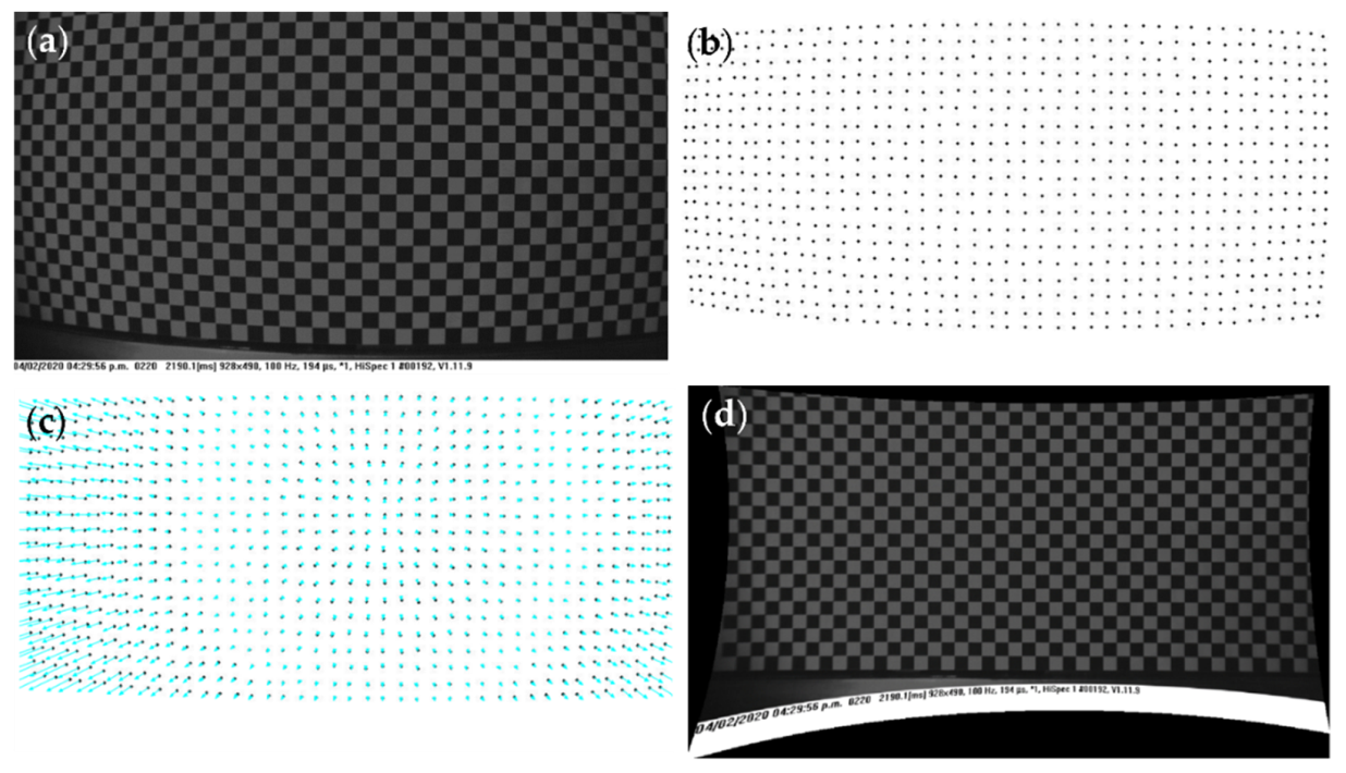
3.1. Stage 1: Calibration and Rectification

The calibration procedure of the acquired images was performed through a pinhole camera model calibration by means of Zhang’s approach [22]. The main objective behind this implementation was to retrieve (a) the intrinsic parameters, (b) the extrinsic parameters, and (c) the distortion coefficients. Then, by employing the pinhole camera model, the images were rectified, the distortions were minimized, and the relationship between pixel and real-world units was obtained.

3.1.1. Image Calibration

The calibration of the camera was performed by means of the well-known pinhole model using a chessboard with squares of 22 mm of length, which was placed on the closest flume wall, as shown in Figure 2a. The main objective behind this task is to determine transformation parameters between an object in a three-dimensional (3D) space and its reprojection to the observed two-dimensional space (2D) from visual information (image). Thus, by considering 3D real-world coordinates for an arbitrary point as X = (X,Y,Z,1)T, its 3D coordinates in a 2D camera image Xcam are transformed by means of the next expression:
X cam = R   t X
where R is a 3 × 3 rotation matrix, and t is a 3 × 1 translation matrix. Assuming x = (x,y,1)T, as the image 3D coordinates, the 3D to 2D mapping is denoted by the next expression:
X = K R   t X
where K is a 3 × 3 matrix of the capturing device with its intrinsic parameters, which in turn is denoted by
K = f x 0 c x 0 f y c y 0 0 1
where fx and fy are the focal length of the capturing device in x and y axes, and (cx, cy) are the principal point coordinates.
To determine the intrinsic and the extrinsic parameters, several images were obtained from a grid of dots with equal spacing. Then, all coordinates of the centroid of the points were found in each image. These coordinates in the image correspond to some coordinates of 3D points in the real world. All collected correspondences were stored, and the calibration parameters were retrieved using the NI Vision Assistant software [23].

3.1.2. Image Rectification

The image rectification is a required stage after determining the camera parameters through calibration since there are different types of distortion in images from pinhole cameras. Two major distortions are the radial and the tangential ones. In the former, straight lines appear curved, seeming that they move away from the center of image. In the latter, the lens plane of the capturing device is not perfectly parallel to the imaging plane; as a result, some regions in the scene may look nearer than expected. Then, to deal with the distortions in the captured images, it is necessary to find the distortion coefficients (k1, k2, k3, p1, and p2). Thus, the radial distortion problem can be solved by using the next two expressions:
x c = x 1 + k 1 r 2 + k 2 r 4 + k 3 r 6
y c = y 1 + k 1 r 2 + k 2 r 4 + k 3 r 6
Similarly, the tangential distortion can be solved by using the next two expressions:
x c = x + 2 p 1 xy + p 2 r 2 + 2 x 2
y c = y + p 1 r 2 + 2 y 2 + 2 p 2 xy
Figure 2 illustrates the main steps of the calibration and the rectification stages of the present work.
Figure 2a,b show the input calibration image and the detected corners from the chessboard square intersections, respectively. Figure 2c includes some arrays that represent the error due to distortion. Figure 2d presents the aspect of the rectified images, which were employed for the purpose of the present work. For an in-depth description and mathematical background of the employed calibration and rectification procedures, the reader is referred to [22,24].

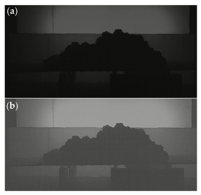
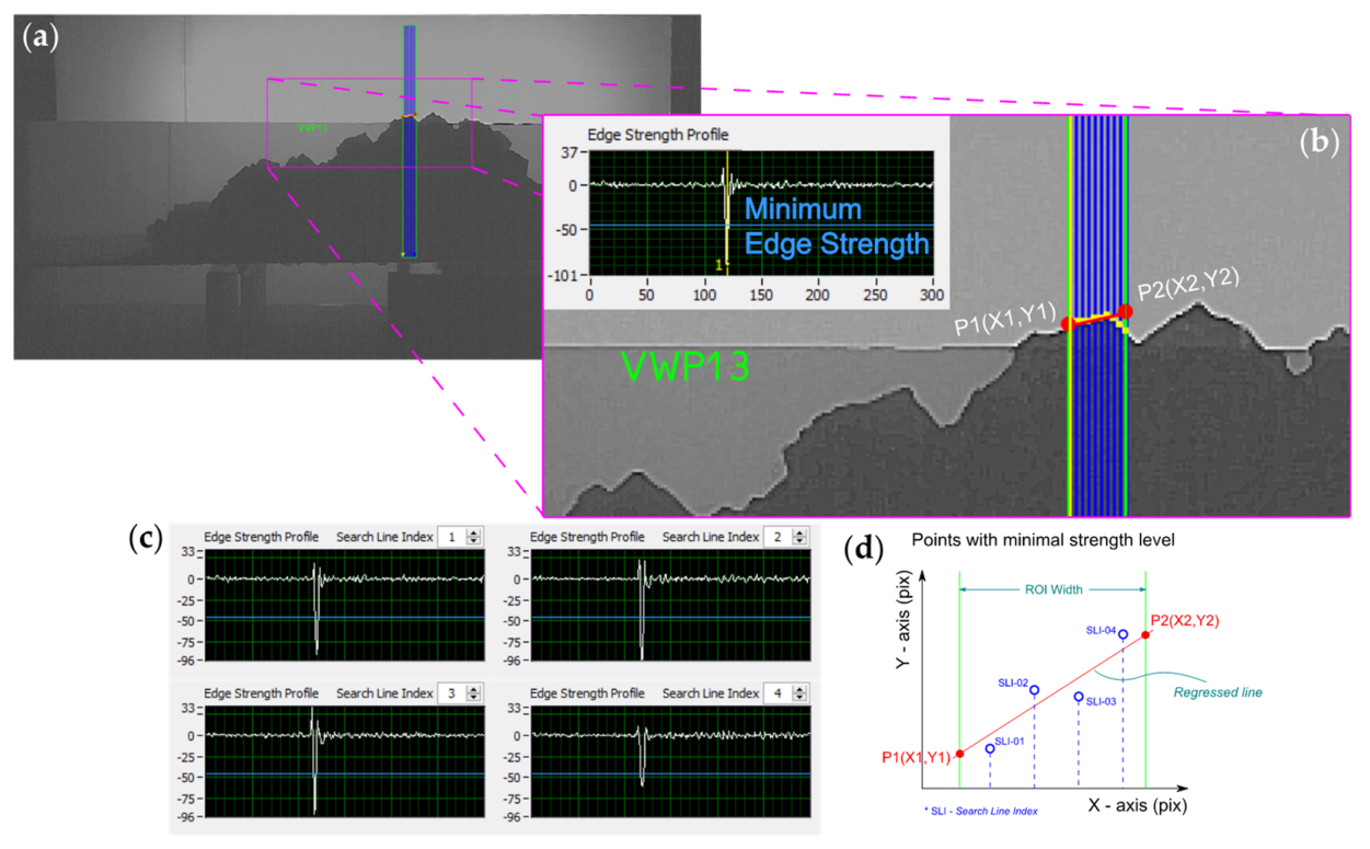
3.2. Image Processing
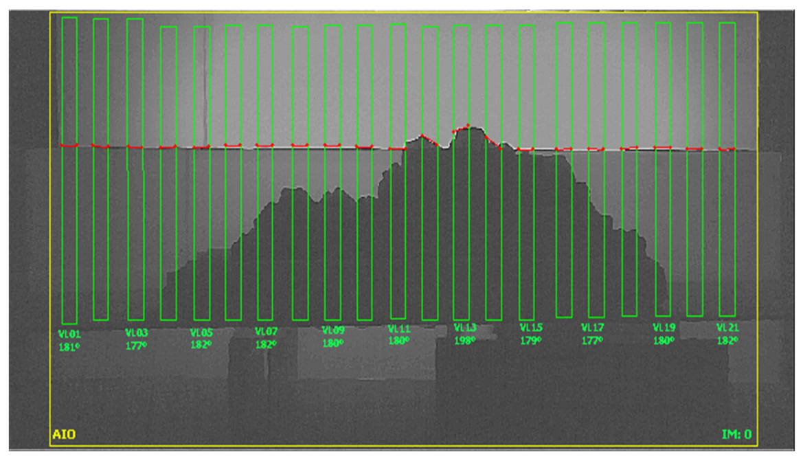
The image processing stage was conducted in three main steps to perform image enhancement in the set of input images before the image analysis. In the first step, the brightness parameters on the scene were modulated by considering, respectively, brightness and contrast levels of 0.52 and 0.18 and a gamma adjust of 0.46. In the second step, a 3-pixel size median filter was applied to the entire stack of modulated images for noise reduction. In the third step, a convolution of the images, with a 3 × 3 kernel, ck = [[−1 −1 −1], [ −1 10 −1], [ −1 −1 −1]], was performed to highlight the details of the images. Figure 3a shows the aspect of the input image, whereas Figure 3b shows the resulting output image, obtained after performing the described image processing stage.

3.3. Image Analysis

For the image analysis, the NI Vision Builder® software [25] was employed. It allowed us to define regions of interest (ROIs), named in this work as virtual level probes (VLs, Figure 4), to track edge motions inside of them. In general, the main objective was to identify straight edges within these regions by seeking the better-defined edge from top to bottom of the ROI [25,26].
As shown in Figure 4, initial and final locations of the edges identified inside each ROI (red lines) are defined to keep their horizontal position in the vertical rectangles that define the VLs. Thus, the main idea consists in tracking the displacement of these edges as the flow is interacting with the structure. To define the water elevation, at specific positions over the horizontal domain, the mean value of the measurements obtained at the start and the end of each edge was considered (see a detailed description of the measuring process in Appendix A). The parameters for straight edge determination considered in NI Vision Builder® were: (i) a minimum edge strength of 10 pixels, (ii) kernel size of 3 pixels, (iii) projection width of 2 pixels, and (iv) gap of 2 pixels. A total of 21 ROIs (VLs) were considered to perform the analyses (Figure 4). These ROIs had a fixed width of 20 mm, a height around 300 mm, and a spacing between them of 20 mm. A brief error analysis of the VL measurements is included in Appendix B.

4. Results and Discussion

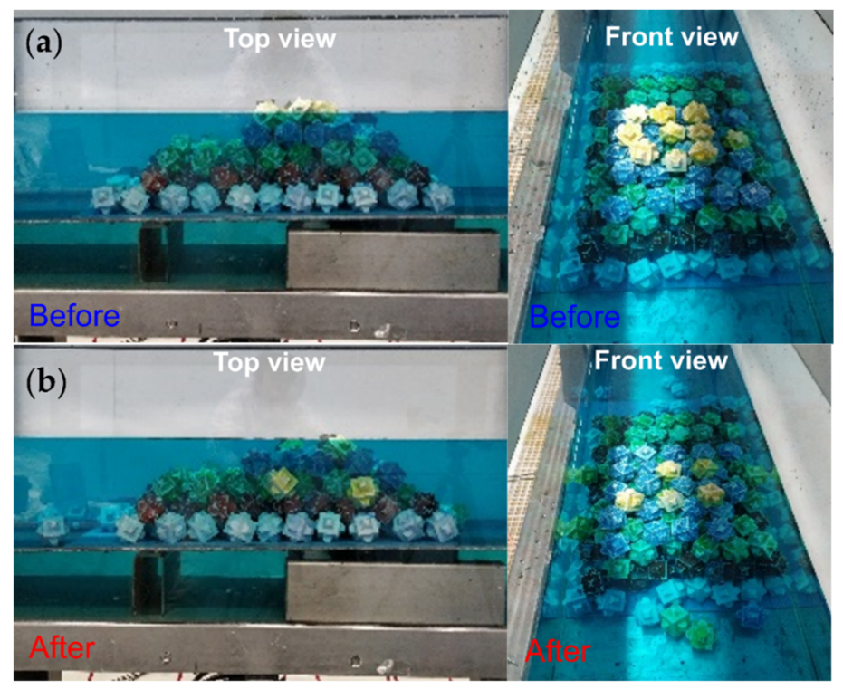
4.1. Qualitative Analysis of the Experiments

In the present experiments, the incident flows interacting with the Cubipod structure were trains of waves that broke just before or during the interaction. After several pretests, it was tented to find the wave train that presented this behavior. Overall, a wave train of 100 waves with 1.5 s of period was considered. These waves caused several displacements of the Cubipods with respect to the initial condition of the structure, as can be observed in Figure 5, which shows top and front views of the structure before (Figure 5a) and after (Figure 5b) the interaction of the waves. As can be observed in Figure 5a, the layers of the structure are characterized by Cubipods of different color, being white in the base and yellow on the top. Note that, at the end of the experiment, there were several armor units extracted from the structure. Alternatively, Figure 6 shows some differences between the initial frame of the video and the subsequent stages. From this figure, it can be clearly inferred, from a two-dimensional point of view, that the elements of the structure suffered some motion during and after the interaction of the wave trains.
The large displacement of the Cubipods from the top of the structure resembles a failure condition of this type of structure. It is important to highlight that this wave condition was generated to test the structure under the action of violent flows. In conventional testing conditions with longer waves, negligible displacements were detected.
To illustrate the strong interactions that the waves had with the structure, Figure 7 shows some snapshots of relevant stages of the first five waves of the wave train. It is important to remember that the wave train was generated with design regular wave parameters (0.66 Hz and 0.65 m of wave frequency and amplitude, respectively). However, these parameters provided a dimensionless depth value kh~0.53 (where k is the wave number and h is the water depth), suggesting intermediate depth conditions (π/10 > kh > π, [27]). In Figure 7, it can be observed that the first and the second waves, which correspond to the ramp function of the signal introduced to the wavemaker, did not break. Next, the third wave presented partially breaking features just above of the structure, whereas the subsequent waves broke just before of it. The snapshots show the features of the waves before, during, and after the interaction with the structure. Note that, when the waves presented breaking features, three dimensional effects could be observed in the free surface, it being complex to define the water level even by visual inspection. The use of the present image-based procedure requires the assumption that the water surface will be identified in the water–air interface, disregarding the differentiation between three-dimensional surface effects. Despite this assumption, this approach can provide useful information for better understanding of the spatio-temporal water evolution, as shown in next sections.

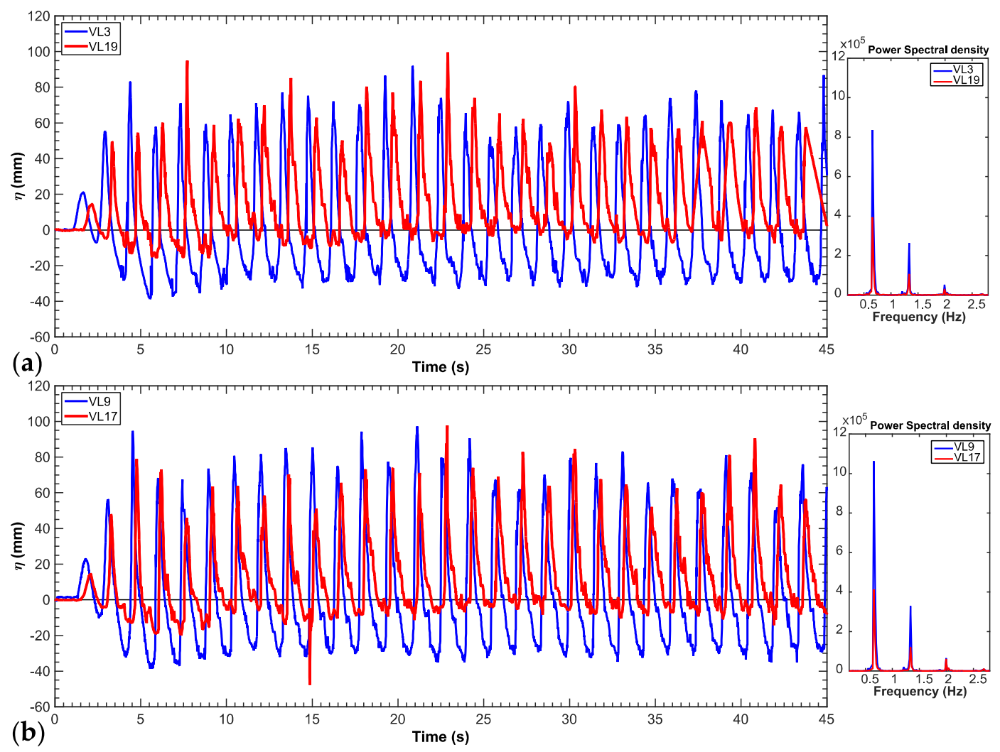
4.2. Water Elevation Analysis

Considering the 2D assumption to analyze the present experiment, the image-based methods can be applied to obtain useful measurements of the variation of the VLs (i.e., red edges in Figure 4). As described in Section 3.3, the measurements can be acquired for initial and final extremes of the edges, which can be helpful to know the instant inclination of the edge. However, to simplify the analysis, only the variation of the middle of the edges has been considered in this study (see Appendix A for details).
Figure 8 shows the spatio-temporal evolution of the detected levels in the 21 VL sensors that were defined in Figure 4, for the duration of 10 s (interaction of the first 6 waves). Note that at the rest condition, before the wave’s incidence, some of the identified edges were those of the Cubipods located at the top of the structure (e.g., VLs 12, 13, and 14). In Figure 8, after the occurrence of each wave, the resultant level of these Cubipods can be observed. Note also that the third wave was the one that reached the highest water levels before the interaction with the structure with respect to the other waves. Although the surface shown in the figure is not a complete reconstruction of the flow evolution because of the 2D assumption, it is a remarkably interesting spatio-temporal representation that could be very useful for analyzing different test configurations.
To have an idea about the effect of the structure on the incident wave elevations, Figure 9 shows a comparison of the water surface measurements provided by the VLs sensors located before and after the structure for most of the waves captured during the camera acquisition time. Hereafter, in the comparisons of time series of water elevations, the power spectral density of the signals is included. It allows identifying the main components of the signals and having an idea about the reduction of wave energy by the structure. In all the comparisons, the main frequency of the incident waves can be identified (~0.66 Hz) as well as additional small peaks for other frequency components, which are, perhaps, due to nonlinear instabilities of the waves (see some examples in [28]) or bound waves in the present test condition. The power spectral density was calculated using the Fast Fourier Transform available in MATLAB, following the procedure described in [29]. Figure 9a presents the comparison for VL3 and VL9, whereas Figure 9b compares VL9 and VL17. Notice that the former are at farther locations from the crest of the structure than VL9 and VL17. In both comparisons, it can be observed that the structure contributed to the reduction of water surface levels of the incident waves. This reduction was observed in most waves for the maximum amplitudes of the crests (~10–20% for most waves), assuming that we are monitoring the upper visible surface, including the breaking flow effects. Similarly, it can be noted that the structure significantly reduces the amplitude of the troughs (more than 60% for most waves).
To analyze more details of the wave surface variations due to the presence of the structure, Figure 10 shows the comparison between measurements of three consecutive probes located before (VL3, VL4, VL5) and after (VL17, VL18, VL19) the structure for 13 waves (0 < t < 20 s). Through these comparisons, it can be inferred that, for the first four waves, the tendency was to increase and decrease their amplitudes when approaching and leaving the crest of the structure, respectively. In the fourth wave, this behavior was conversely observed; the wave reduced the amplitudes before the interaction, increasing in the flow passing the structure. This behavior may be attributed to the failure of the Cubipod at the crest of the structure, as described in the next subsection. For the aftercoming waves, the maximum elevations after the structure presented irregular trends, tending to increase in some cases as water moved away from the structure. This trend may be partially related to the changes in the arrangement of the Cubipods at the crest (Section 4.3).

4.3. Identification of Structure Failure

With the present approach, it was also possible to identify the interface (edge) between the Cubipod located at the crest of the structure and the air, as described in Section 3.3. In this study, these edges were identified inside VL13, VL14, and VL15 (see the red edges in Figure 4) when the wave was not over the structure. When the wave was above the crest Cubipods, detected edges corresponded to the surface of the waves. Thus, knowing the variation of the Cubipods edge after each wave interaction can be useful to identify the instants at which Cubipods present significant displacements. Drastic changes could be useful to analyze possible failure conditions on this type of structures, particularly at the top.
Figure 11 shows the comparison of edge displacement measured by VL13, VL14, and VL15, including some snapshots to illustrate relevant stages during the wave–structure interactions. These measurements correspond to the vertical position of the middle of the edge inside the VL sensors, as described in Section 3.3 and Appendix A. It can be observed that, after the first two waves, the VLs of the Cubipods remained unchanged. However, after the third wave, these levels presented drastic changes for VL14 and VL5, suggesting a failure condition in some Cubipods. After the fourth wave, the levels at VL14 seemed to maintain an almost invariable amplitude, whereas those at VL15 presented more variations. The snapshots below the graph can illustrate these stages during the interaction.
It is particularly important to quantify the performance of the structure before and after failure of the top members. With the present approach, this can be analyzed in a simplified way, assuming two-dimensional flow and water elevation measurements taken upstream and downstream of the structure during the failure stage. Thus, Figure 12 shows a comparison of VL6 against VL18 measurements taken during the first five waves, including the failure stage shown in Figure 11. Note that, before failure, the structure performed well in minimizing the maximum wave amplitudes (crest amplitudes). However, after failure, it is clearly observed that the structure did not contribute to reduce this maximum. For the subsequent waves, performance of the structure to reduce the wave crests was more noticeable.

5. Conclusions

In this work, we proposed an alternative and simplified image-based approach to investigate wave–structure interaction in wave flume experiments. The approach is two-dimensional and based in the stages of image acquisition, processing, and analysis of gray-scale images obtained with a conventional camera. The novelty of this approach is the use of virtual level (VL) measurements to investigate the water evolution before and after the structure and to detect some displacements of the elements of the structure. The VL approach consists in defining region of interests at specific locations along the horizontal scale of the image. Then, edge interfaces (levels) are detected for both the water surface and the structure top elements. Next, the displacement of these levels is tracked to perform VL measurements. This approach allows investigating the spatio-temporal evolution of the VL variation under a two-dimensional assumption. To demonstrate the applicability of the method to investigate the interaction of breaking waves with a Cubipod homogeneous low-crested coastal structure, it was possible to conclude the next findings:
  • Drastic changes identified in the levels of the Cubipods interfaces (edges) can be useful to investigate failure modes in similar structure configurations.
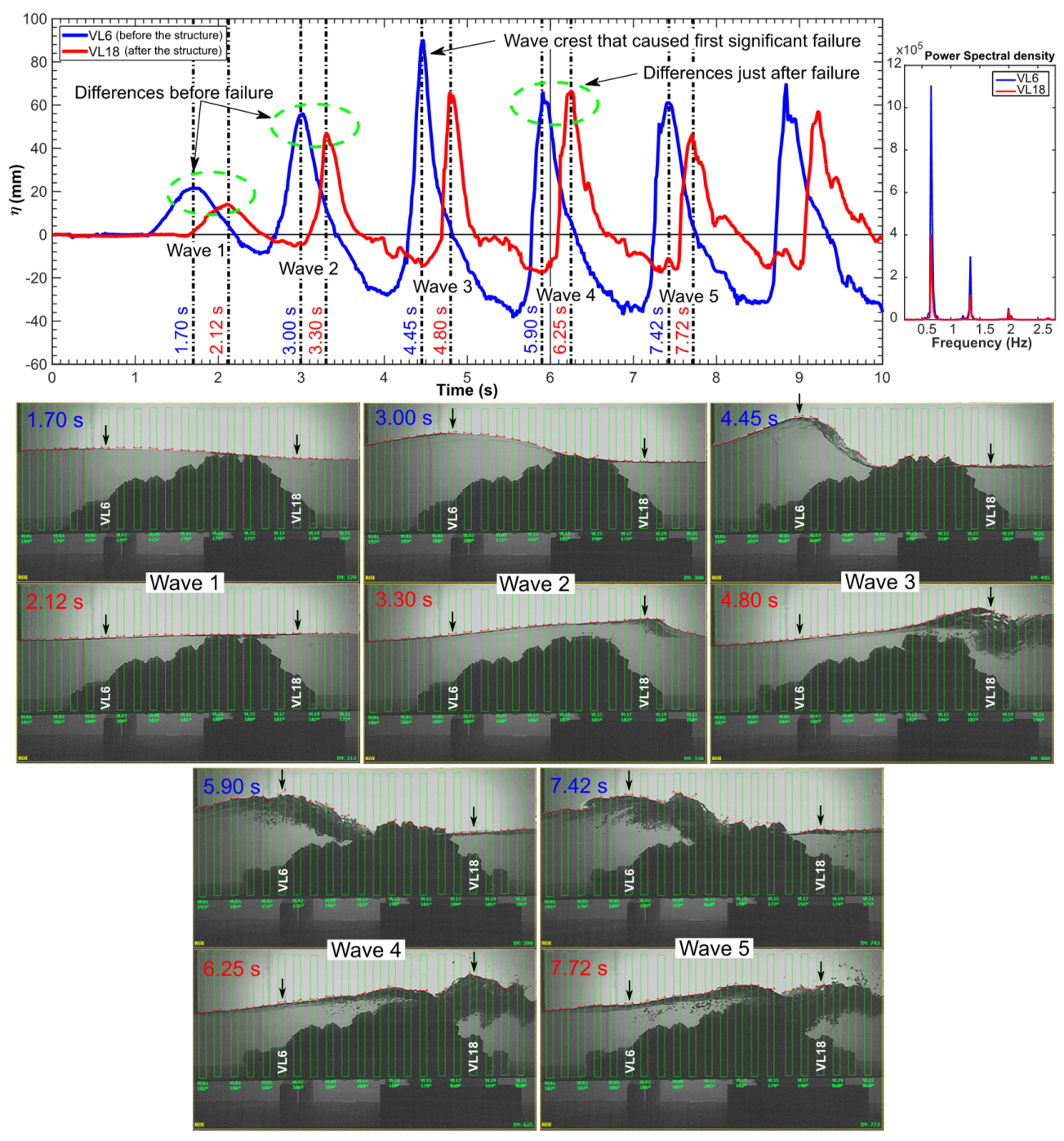
  • The failure of the Cubipods at the crest showed the decreased performance of the structure to reduce the incoming wave elevations.
  • The water elevation data that can be obtained with this approach before and after the structure can be useful to perform comparisons with analytical or numerical models.
  • Although it is complex to build identical structure models as the one presented in this work, limiting systematic analysis, the present image-based approach can be extended to analyze a wide range of wave flume configurations. In this research, the internal memory of the camera was used. By increasing this memory, the approach can be further used to analyze breakwater behavior in irregular sea.
  • The use of color cameras, the application of improved image enhancement methods, and the definition of VLs of different sizes at specific locations could be helpful to identify and monitor the displacement of different interfaces.

Author Contributions

Conceptualization: J.V.H.-F., I.D.H., E.M., and M.E.; methodology: M.E., J.V.H.-F., and I.D.H.; software: I.D.H., J.V.H.-F.; validation: M.E., J.V.H.-F., I.D.H., and E.M.; formal analysis: M.E., J.V.H.-F., I.D.H.; investigation: M.E., J.V.H.-F., I.D.H., and E.M.; resources: E.M., and I.D.H.; data curation: J.V.H.-F., I.D.H.; writing—original draft preparation: M.E., J.V.H.-F., I.D.H., and E.M.; writing—review and editing: M.E., J.V.H.-F., I.D.H., and E.M.; visualization: M.E., J.V.H.-F.; supervision: E.M.; project administration: M.E., and E.M.; funding acquisition: E.M. All authors have read and agreed to the published version of the manuscript.

Funding

This research was funded by the CONACYT-SENER-Sustentabilidad Energética project: FSE-2014-06-249795 “Centro Mexicano de Innovación en Energía del Océano (CEMIE-Océano)”.

Institutional Review Board Statement

Not applicable.

Informed Consent Statement

Not applicable.

Data Availability Statement

The data presented in this study are openly available in http://0-dx-doi-org.brum.beds.ac.uk/10.17632/ny24d49wkd.1.

Acknowledgments

Authors wish to thank the staff of the Coast and Ports Laboratory Engineering Institute, National Autonomous University of Mexico for the technical help.

Conflicts of Interest

The authors declare no conflict of interest.

Appendix A. Virtual Level Definition

It is important to mention that the present methodology to employ virtual level (VL) measurements in coastal structures experiments can be extended to different setup configurations. Therefore, there are some aspects that should be taken into account with respect to image processing and analysis (measuring) stages.
As described in Section 4.2, the present approach considers the location of the best-defined interface contour (edge) within a specific region of interest (ROI). To do this, the algorithm needs the user to define the ROI and the minimum edge strength.
Figure A1 illustrates the measuring principle scheme for the virtual level of the 13th ROI. Within the ROI, several search lines (see blue lines) are defined by means of a constant gap between them (Figure A1a,b), allowing a top-to-bottom mapping of the changes on both contrast and intensity levels along the profile traced by each line. If a change higher than the minimum edge strength requested is detected (using absolute values), as shown in Figure A1c, then a regression point is defined between horizontal and vertical coordinates (Figure A1d). This procedure is repeated for each search line in the ROI and ends with a regression line that fits the regression points (Figure A1d). The intersections of the regression line with the ROIs boundaries define the extreme points of the virtual level, whereas the middle coordinate of this line defined the level magnitude. Complementary details can be found in [23].
Figure A1. Sketch that illustrates the level measurement procedure for the 13th region of interest (ROI): (a) typical frame and definition of the 13th ROI; (b) search lines (in blue) defined inside the ROI; (c) edge strength profiles of some search lines; (d) definition of the virtual level inside the ROI, which corresponds to a regression line of the search line index points.
Jmse 09 00230 g0a1

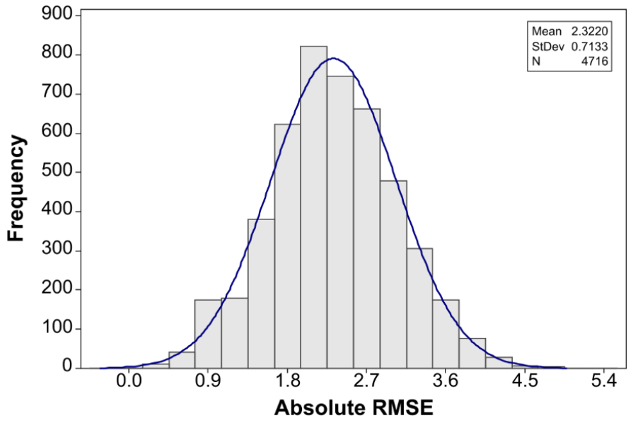
Appendix B. Reliability Analysis of the VL Measurements

The reliability of the approach employed highly depends on the algorithm’s ability to detect the variation in contrast and intensity levels. Thus, in underexposed or overexposed captures, these parameters do not vary perceptibly so that no point in the regression (Figure A1d) could be recovered and the detection of the virtual level would be unfeasible. Then, to minimize this as much as possible, it is recommended to apply an equalization of intensity levels to the entire set of images before processing. In this work, the instances in which it was not possible to recover any straight line within an ROI were declared as null values using numeric NaN in the exported files.
To assess the reliability of reported measures, the error in the level measurements from virtual probes can be estimated by considering that the actual vertical location of the i-th level (Ŷ, i.e., the measured level inside a ROI), at instant t, will be within the range of Y1[t][i] ≤ Ŷ[t][i] ≤ Y2[t][i], where Y1 and Y2 denote the vertical coordinates of the points where the regressed line intersects the ROIs boundaries, and Ŷ is the current registered vertical level magnitude. Thus, the root-mean square error (RMSE) of all the measurements in each instant can be measured by using the absolute difference with one of the vertical coordinates of P1 and P2 (see Figure A1d), as described by expression (A1).
RMSE t = Y ^   Y 2 N = i = 1 N Y ^ t i Y 2 t i 2 N
Then, by collecting all the absolute RMSE values from all the frames, the error deviation can be estimated by means of a normal distribution of the collected errors (see Figure A2). The results of the error distribution reported an RMSE ranging from −2.32 mm to 2.32 mm in the measures with a standard deviation of 0.8 mm. These statistics were retrieved from all the 4716 frames (i.e., the video duration, 47.16 s) of the case study.
Figure A2. Normal distribution of the root-mean squared error of virtual level measurements.
Jmse 09 00230 g0a2
The meaning of the presented statistics denotes that reported measures may have a maximum error (RMSE) of ±2.32 ± 0.72 mm. Thus, the measurement approach can be assumed as reliable to be employed in similar problems since the previous indications were considered prior image processing. It is important to mention that the employed approach takes advantage of the built-in functions of a commercial software (NI Vision), but all the steps are possible to be ported in an open-source software such as ImageJ or an object-oriented programming language such as JAVA or Python through the OpenCV libraries.

References

  1. Campos, Á.; Sanchez, M.R.; Castillo, E. Damage in Rubble Mound Breakwaters. Part II: Review of the Definition, Parameterization, and Measurement of Damage. J. Mar. Sci. Eng. 2020, 8, 306. [Google Scholar] [CrossRef]
  2. Douglas, S.; Cornett, A.; Nistor, I. Image-Based Measurement of Wave Interactions with Rubble Mound Breakwaters. J. Mar. Sci. Eng. 2020, 8, 472. [Google Scholar] [CrossRef]
  3. Lopes, H.; Pinto, F.T.; Gomes, F.V.; Cabral, J.; Gadelho, J.; Neves, M.; Reis, M. Laboratory Techniques-Image Processing Tools on Physical Model Tests. In Proceedings of the 6th SCACR International Short Course/Conference on Applied Coastal Research, Lisbon, Portugal, 4–7 June 2013. [Google Scholar]
  4. Viriyakijja, K.; Chinnarasri, C. Wave Flume Measurement Using Image Analysis. Aquat. Procedia 2015, 4, 522–531. [Google Scholar] [CrossRef]
  5. Gómez-Martín, M.E.; Medina, J.R. Wave-To-Wave Exponential Estimation of Armor Damage Progression. In Coastal Engineering; World Scientific: Singapore, 2004; Volume 4, pp. 3592–3604. [Google Scholar]
  6. Vidal, C.; Martín, F.L.; Negro, V.; Gironella, X.; Madrigal, B.; García-Palacios, J. Measurement of Armor Damage on Rubble Mound Structures: Comparison Between Different Methodologies. Coast. Struct. 2003 2004, 189–200. [Google Scholar] [CrossRef]
  7. Gómez-Martín, M.E.; Medina, J.R.; Franco, L.; Tomasicchio, G.R.; Lamberti, A. Cubipod Concrete Armour Unit and Heterogeneous Packing. In Coastal Structures 2007; World Scientific Pub. Co. Pte. Lt.: Singapore, 2009; Volume 2, pp. 140–151. [Google Scholar]
  8. Gómez-Martín, M.E.; Medina, J.R.; Smith, J.M. Damage Progression on Cube Armored Breakwaters. In Coastal Engineering 2006; World Scientific Pub. Co. Pte. Lt.: Singapore, 2007; Volume 5, pp. 5229–5240. [Google Scholar]
  9. Lomonaco, P.; Vidal, C.; Medina, J.R.; Gomez-Martin, M.E. Evolution of Damage on Roundheads Protected with Cube and Cubipod Armour Units. Coast. Mar. Struct. Break. 2009, 1, 169–180. [Google Scholar]
  10. Lemos, R.; Reis, M.T.; Fortes, C.J.; Peña, E.; Sande, J.; Figuero, A.; Alvarellos, A.; Laiño, E.; Santos, J.; Kerpen, N. Measuring Armour Layer Damage in Rubble-Mound Breakwaters under Oblique Wave Incidence. Coast. Struct. 2019, 295–305. [Google Scholar] [CrossRef]
  11. Kocaman, S.; Ozmen-Cagatay, H. The Effect of Lateral Channel Contraction on Dam Break Flows: Laboratory Experiment. J. Hydrol. 2012, 432, 145–153. [Google Scholar] [CrossRef]
  12. Hernández-Fontes, J.V.; Esperança, P.d.T.T.; Graniel, J.F.B.; Sphaier, S.H.; Silva, R. Green Water on A Fixed Structure Due to Incident Bores: Guidelines and Database for Model Validations Regarding Flow Evolution. Water 2019, 11, 2584. [Google Scholar] [CrossRef] [Green Version]
  13. Hernández-Fontes, J.V.; Hernández, I.D.; Mendoza, E.; Silva, R. Green Water Evolution on a Fixed Structure Induced by Incoming Wave Trains. Mech. Based Des. Struct. Mach. 2020, 1–29. [Google Scholar] [CrossRef]
  14. Hernández, I.D.; Hernández-Fontes, J.V.; Vitola, M.A.; Silva, M.; Esperança, P.T. Water Elevation Measurements Using Binary Image Analysis for 2d Hydrodynamic Experiments. Ocean Eng. 2018, 157, 325–338. [Google Scholar] [CrossRef]
  15. Hernández-Fontes, J.V.; Hernández, I.D.; Silva, R.; Mendoza, E.; Esperança, P.T.T. A Simplified and Open-Source Approach for Multiple-Valued Water Surface Measurements in 2D Hydrodynamic Experiments. J. Braz. Soc. Mech. Sci. Eng. 2020, 42, 623. [Google Scholar] [CrossRef]
  16. Medina, J.; Gómez-Martín, M.E.; Mares-Nasarre, P.; Odériz, I.; Mendoza, E.; Silva, R. Hydraulic Performance of Homogeneous Low-Crested Structures. Coast. Struct. 2019, 2019, 60–68. [Google Scholar]
  17. Odériz, I.; Mendoza, E.; Silva, R.; Medina, J. Hydraulic Performance of a Homogeneous Cubipod Low-Crested Mound Breakwater. In Proceedings of the 7th International Conference on the Application of Physical Modelling in Coastal and Port Engineering and Science (Coastalab18), Cantabria, Spain, 22 May 2018. [Google Scholar]
  18. Medina, J.R.; Gomez-Martin, M.E.; Mares-Nasarre, P.; Escudero, M.; Oderiz, I.; Mendoza, E.; Silva, R. Homogeneous Low-Crested Structures for Beach Protection in Coral Reef Areas. In Proceedings of the Coastal Engineering Proceedings; Coastal Engineering Research Council: Sydney, Australia, 2020; p. 59. [Google Scholar]
  19. Maiden, M.D.; Franco, N.A.; Webb, E.; El, G.; Hoefer, M.A. Solitary Wave Fission of a Large Disturbance in a Viscous Fluid Conduit. J. Fluid Mech. 2020, 883. [Google Scholar] [CrossRef] [Green Version]
  20. Trillo, S.; Deng, G.; Biondini, G.; Klein, M.; Clauss, G.F.; Chabchoub, A.; Onorato, M. Experimental Observation and Theoretical Description of Multisoliton Fission in Shallow Water. Phys. Rev. Lett. 2016, 117, 144102. [Google Scholar] [CrossRef] [PubMed]
  21. Fastec-Imaging HiSpec 1 Innovative Low-Light High-Speed Camera 2020. Available online: https://www.fastecimaging.com/wp-content/uploads/2018/05/hispec1.pdf (accessed on 19 December 2020).
  22. Zhang, Z. A Flexible New Technique for Camera Calibration. IEEE Trans. Pattern Anal. Mach. Intell. 2000, 22, 1330–1334. [Google Scholar] [CrossRef] [Green Version]
  23. NI. National Instruments Vision Assistant; Version 2014; NI: Austin, TX, USA, 2014; Available online: https://www.ni.com/pdf/manuals/373379h.pdf (accessed on 11 February 2021).
  24. Wang, Y.M.; Li, Y.; Zheng, J.B. A Camera Calibration Technique Based on OpenCV. In Proceedings of the 3rd International Conference on Information Sciences and Interaction Sciences, Chengdu, China, 23–25 June 2010; pp. 403–406. [Google Scholar]
  25. Lee, J.; Haralick, R.; Shapiro, L. Morphologic Edge Detection. IEEE J. Robot. Autom. 1987, 3, 142–156. [Google Scholar] [CrossRef]
  26. Marr, D.; Hildreth, E. Theory of Edge Detection. Series, B. Biological Sciences; The Royal Society: London, UK, 1980; Volume 207, pp. 187–217. [Google Scholar]
  27. Kennedy, A. Fundamentals of Water Waves. In Encyclopedia of Water: Science, Technology, and Society; Wiley: Hoboken, NJ, USA, 2019; pp. 1–7. [Google Scholar]
  28. Saprykina, Y.V.; Kuznetsov, S.; Smith, J.M. Nonlinear Mechanisms of Formation of Wave Irregularity on Deep and Shallow Water. In Coastal Engineering 2008; World Scientific Pub. Co. Pte. Lt.: Singapore, 2009; Volume 5, pp. 357–369. [Google Scholar]
  29. MathWorks MathWorks: FFT for Spectral Analysis. Available online: https://la.mathworks.com/help/matlab/math/fft-for-spectral-analysis.html (accessed on 15 January 2021).
Figure 1. Experimental setup: (a) front and top photo views of the Cubipod homogeneous low-crested structure (HLCS); (b) sketches of front and top views of the wave flume and the structure location, including dimensions; (c) details of the geometric characteristics of the front view of the Cubipod structure; (d) top view of the designed placement grid for the bottom layer of the Cubipod armors.
Jmse 09 00230 g001
Figure 2. Stages during image calibration and rectification: (a) input calibration image; (b) detected corners; (c) error estimation; (d) image calibration and rectification.
Jmse 09 00230 g002
Figure 3. Image processing enhancements: (a) input image; (b) enhanced image.
Jmse 09 00230 g003
Figure 4. Definition of the 21 virtual level (VL) probes to perform the measurements of the identified edges. The degree values indicate the angle of the identified edges (in red) with respect to the horizontal.
Jmse 09 00230 g004
Figure 5. Initial and final stages of the structure before and after the interaction of the breaking incident waves: (a) top and front views of the initial shape of the structure; (b) top and front views at the end of the experimental test.
Jmse 09 00230 g005
Figure 6. Differences between the initial frame of the videos and the frames of subsequent stages to demonstrate variations of the structure.
Jmse 09 00230 g006
Figure 7. Features of the first six incident waves interacting with the structure. For waves 3 to 6, snapshots of the stages before (left column), during (middle column), and after (right column) the interaction are shown.
Jmse 09 00230 g007
Figure 8. Spatio-temporal evolution of the vertical displacement of the detected levels (η) of the first six incident waves. The elevations are shown for the 21 virtual level probes (VLs) distributed along the entire horizontal domain of the image data, considering the time 0 < t < 10 s. The color bar in the right side indicates the magnitudes of the displacements.
Jmse 09 00230 g008
Figure 9. Comparisons of water elevations (η) measured before and after the interaction of the incident wave trains with the structure, including the power spectral density of the signals: (a) comparison of VL3 (located at the beginning of the horizontal image domain) with VL19 (located at the end of the domain); (b) comparison of VL9 (located close to the structure, before the top) with VL17 (located close to the structure, after its top).
Jmse 09 00230 g009
Figure 10. Comparison of water elevations (η) measured by three consecutive virtual level (VLs) sensors placed before the structure (VL3, VL4, and VL5) with three consecutive VLs located after the structure (VL17, VL18, and VL19), including the power spectral density of the signals.
Jmse 09 00230 g010
Figure 11. Detection of failure of the Cubipods located at the top of the structure through the analysis of virtual levels (VLs). Above: comparison of the edge displacement measurements taken by the VLs 13, 14 and 15, which were placed on the structure, including the power spectral density of the signals. When water moved inside these VLs, they detected the upper water surface. When the wave passed, the VLs detected the edge of the Cubipods located at the top of the structure. Below: representative snapshots at different time instants.
Jmse 09 00230 g011
Figure 12. Above: comparison of water elevations measured by the virtual level (VL) sensors VL6 and VL18, located just before and after the structure, respectively, during the first interactions of waves with the structure. The power spectral density of the signals is included. Below: snapshots representative of the maximum elevations measured by these sensors.
Jmse 09 00230 g012
Table 1. Geometric parameters of the Cubipod HLCS.
ScaleCrown Width (m)Base Width (m)Structure Height (m)Number of Rows of the 5-Layer Cross-Section
1:42.80.160.610.1911 + 9 + 8 + 5 + 3
Publisher’s Note: MDPI stays neutral with regard to jurisdictional claims in published maps and institutional affiliations.

