Coupled Level-Set and Volume of Fluid (CLSVOF) Solver for Air Lubrication Method of a Flat Plate

Abstract

With the implementation of the energy efficiency design index (EEDI) by the International Maritime Organization (IMO), the goal of which is to reduce greenhouse gas (GHG) emissions, interest in energy saving devices (ESDs) is increasing. Among such ESDs are air lubrication methods, which reduce the frictional drag of ships by supplying air to the hull surface. This is one of the efficient approaches to reducing a ship’s operating costs and making it environmentally friendly. In this study, the air lubrication method on a flat plate was studied using computational fluid mechanics (CFD). OpenFOAM, the open-source CFD platform, was used. The coupled level-set and volume of fluid (CLSVOF) solver, which combines the advantages of the level-set method and the volume of fluid method, was used to accurately predict the air and water interface. Rayleigh–Taylor instability was simulated to verify the CLSVOF solver. The frictional drag reduction achieved by the air lubrication of the flat plate at various injected airflow rates was studied, and compared with experimental results. The characteristics of the air and water interface and the main factors affecting the cavity formation were also investigated.

1. Introduction

As global warming accelerates due to greenhouse gas (GHG) emissions, the international community remains vigilant. The International Maritime Organization (IMO) has imposed regulations on GHG emission and energy efficiency design index (EEDI) to ships built from 2013. Based on emissions in 2008, the aim was to reduce carbon emissions by 10% from 2016, 20% from 2020, and 30% from 2025. Accordingly, energy-saving devices (ESDs) are being actively studied as a means of increasing the fuel efficiency of ships [1,2,3]. For ships with a high Froude number, studies on ESDs that reduce frictional drag are particularly active.

In the past, research on reducing the frictional drag has examined the riblet method [4] and the flexible wall method [5] as approaches to decreasing the velocity gradient on the hull surface. However, these methods were vulnerable to damage, and had the disadvantages of causing environmental pollution.

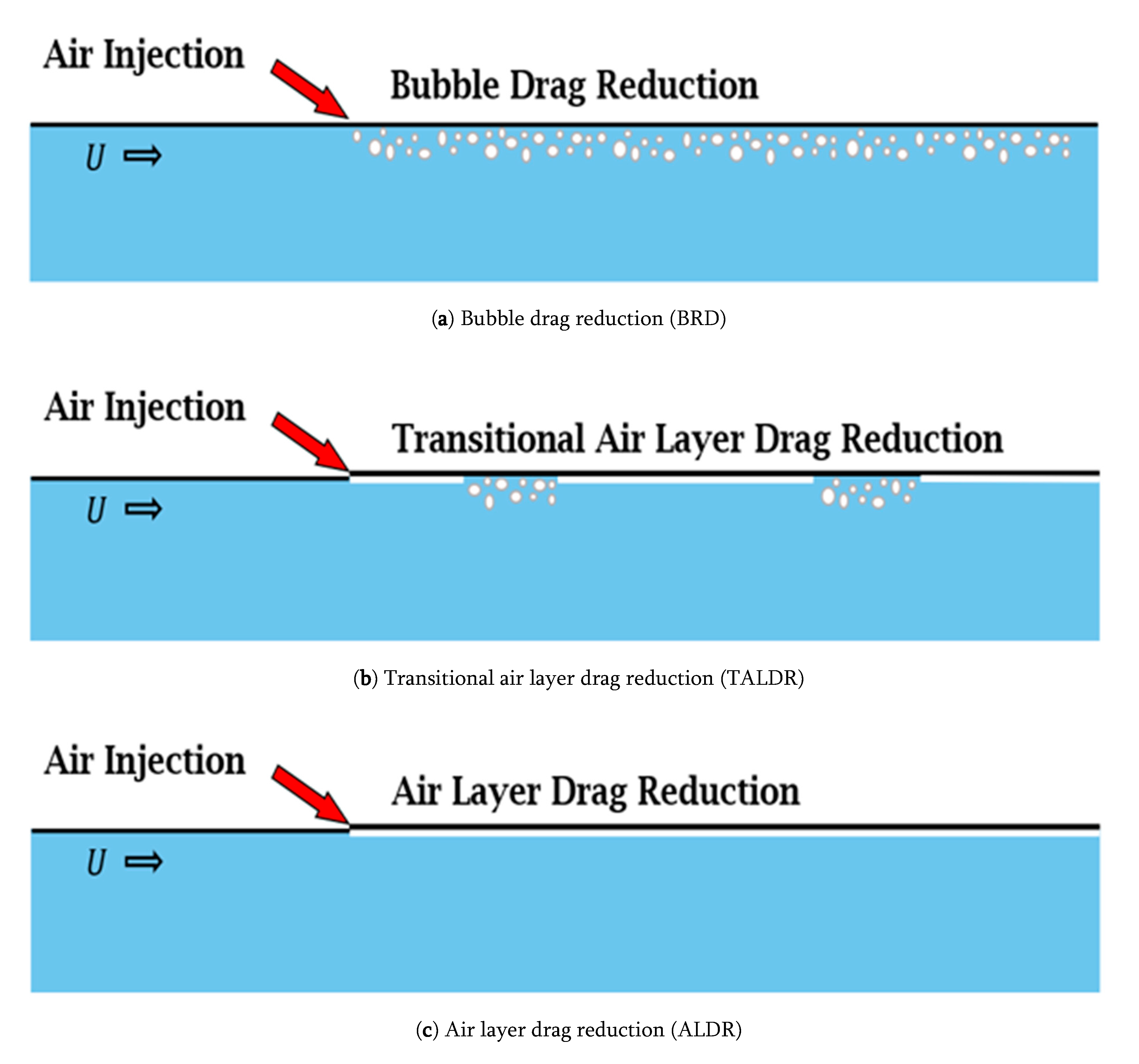
Recently, an air lubrication method in which air is injected at the flat bottom of a ship to reduce the frictional drag has been actively studied. The air lubrication method reduces the frictional drag through the injection of air on the hull bottom surface to form an air layer, thereby reducing the submerged surface area of ships. As shown in Figure 1, the shape of the air layer can be broadly divided into three categories: bubble drag reduction (BDR), transitional air layer drag reduction (TALDR), and air layer drag reduction (ALDR). In the BDR regime, the injected air forms air bubbles, and the frictional drag reduction is not high. On the other hand, in the ALDR regime, an air layer is continuously formed at the surface, and the frictional drag reduction is higher. The TALDR regime is a mix of these two states. The air lubrication method is advantageous, in that the reduction in fuel cost that can be achieved by lowering the frictional drag is higher than the cost of installing and operating the device [6]. Currently, a range of air lubrication systems is being applied to actual ships. In sea trials, the Mitsubishi Air Lubrication System (MARS) of Mitsubishi Heavy Industries achieved a fuel savings up to 12% [7]. In 2018, Samsung Heavy Industries installed “Samsung Advanced Vibration and Energy Reduction (SAVER) Air”, an air lubrication system, resulting in a 4% fuel savings [6]. Daewoo Shipbuilding and Marine Engineering also applied its own DSME ALS to LNG carriers in 2019. It has been confirmed that the air lubrication method is effective in terms of fuel-saving and environmental benefits.

In addition to the utilization of the air lubrication system for ships, many studies have been carried out on the physical characteristics of injected air. To exclude the effect of shape, studies have been conducted on air lubrication on a flat plate [9,10,11]. Hao [12] studied the effect of ship motions by the air layer. Kim et al. [13] predicted the full-scale resistance of a ship with an air lubrication method and captured the air layer using the volume of fluid (VOF) method. There have been some challenges in simulating the VOF method. Kim et al. [14] analyzed the air lubrication method using the VOF and Eulerian multiphase (EMP) methods. In some studies, the VOF method has limitations when it comes to reproducing the behavior of the air layer in the BDR or TALDR regimes [14].

The VOF method has the advantage of achieving better mass conservation, but has a disadvantage due to difficulty in accurately predicting the radius of curvature of the interface in a region in which the volume ratio is discontinuous. A level-set, another method of tracking the interface, has the advantage of having high accuracy with regard to the radius of curvature, but the disadvantage of difficulty preserving mass. To overcome those difficulties, the coupled level-set and volume of fluid (CLSVOF) method, which combines the advantages of the VOF method and the level-set method, was proposed [15]. In a similar study, a continuum surface force (CSF) was developed that considered surface-tension force in the VOF method [16]. Albadawi [17] proposed a simple coupled level-set and volume of fluid (S-CLSVOF) that combined the two methods using the CSF. The CLSVOF method is applied in a wide range of engineering fields. Dianat et al. [18] selected the CLSVOF method to study liquid droplets over solid surfaces, which could be applied to exterior water management on road vehicles. Li et al. [19] simulated gas-assisted injection modeling process by the CLSVOF method.

The objectives were (1) to develop the CLSVOF solver and (2) to apply it to an air lubrication system of a flat plate. The CLSVOF solver was developed using open source computational fluid dynamics libraries, called OpenFOAM version 6.

2. Model Description

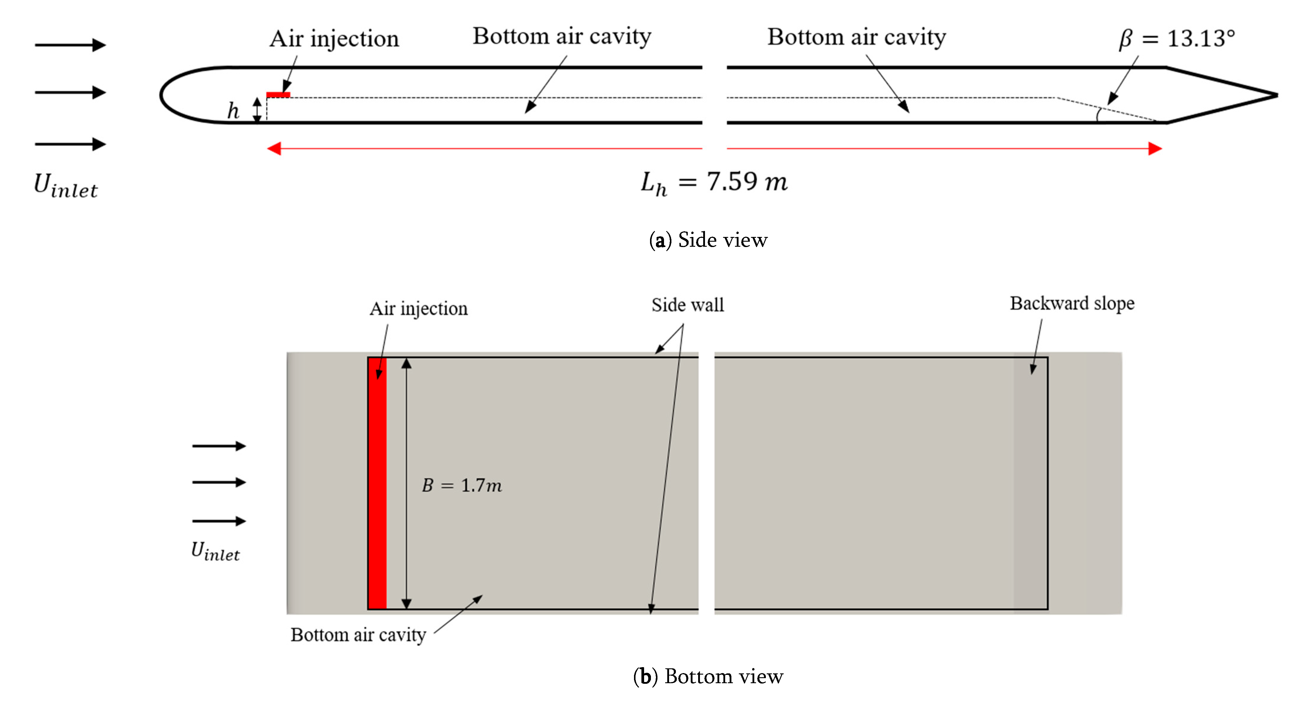
A flat plate with a length of 8.19 m, a breadth of 1.71 m, and a height of 0.06 m were selected. The bottom air cavity to trap the air had a length of 7.59 m, a width of 1.7 m, and a height of 0.035 m. At both sides of the bottom air cavity, a thin plate with a breadth of 0.005 m was installed. Figure 2 shows the flat plate employed in this present study. The air was injected from the air injection in the bottom air cavity. The computations were carried out with the Reynolds number of $1.1\times {10}^7$ and the Froude number of $0.173$.

Table 1. Test cases.

	${\mathit{C}}_{\mathit{q}}$	${\mathit{Q}}_{\mathit{a}\mathit{i}\mathit{r}}\mathit{ }\left({\mathit{m}}^3/\mathit{s}\right)$
Case 1	0.037	0.0152
Case 2	0.074	0.0304
Case 3	0.112	0.0461
Case 4	0.149	0.0614
Case 5	0.180	0.0742

lists the test cases for various injected airflow rates. The coefficient of the injected air flow rate ($C_q$) and the reduction ratio of the total drag (${\eta }_T$) can be expressed as:

$$C_q=\frac{Q_{air}}{VBh}$$

(1)

$${\eta }_T=\frac{R_{T_0}-R_T}{R_{T_0}}\times 100(\%)$$

(2)

where $Q_{air}$ is the flow rate of the injected air, V is the inlet flow velocity, B is the width of the flat plate, and h is the height of the bottom air cavity. The subscript “w/o air” and “w/ air” indicate the cases without injected air and with injected air, respectively.

3. Computational Methods

3.1. Governing Equations

The mass and momentum-conservation equations in the incompressible flow could be written as

$$\nabla ·\overrightarrow{U}=0$$

(3)

$$\frac{\partial \overrightarrow{U}}{\partial t}+\left(\overrightarrow{U}·\nabla \right)\overrightarrow{U}=-\nabla p+\nabla ·\left(\nu +{\nu }_T\right)\left(\nabla \overrightarrow{U}+\nabla {\overrightarrow{U}}^T\right)$$

(4)

where $\overrightarrow{U}$ is the velocity vector, $p$ is the pressure, $\nu$ is the kinematic viscosity, and ${\nu }_t$ is the turbulent kinematic viscosity.

To close the Reynolds stress term, $k-\omega SST$ model was selected [20]. The $k-\omega SST$ model is a hybrid model combining the $k-\omega$ model in the near wall and the $k-\epsilon$ model in the freestream.

3.2. Interface Capturing Method

3.2.1. VOF Method

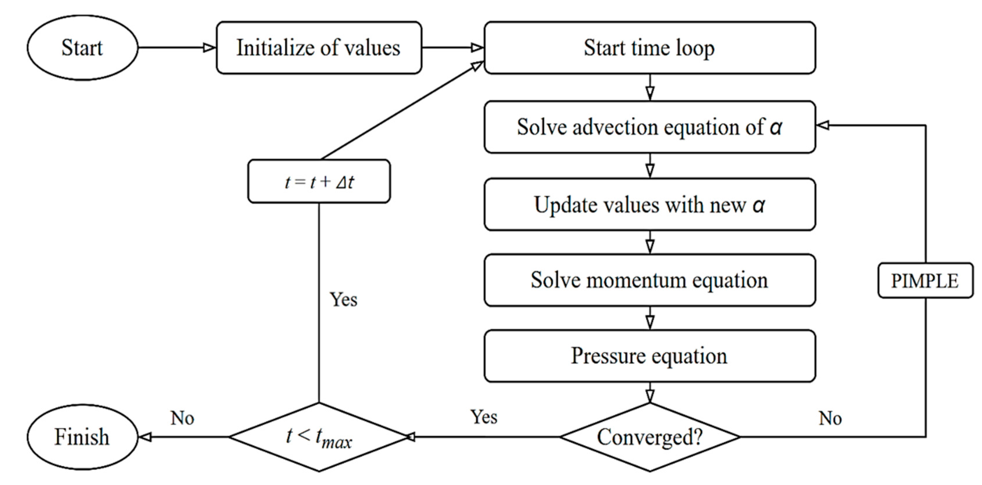
The volume of fluid (VOF) method is a front capturing method that defines the interface using the volume fraction of each cell and expresses the shape and motion of the interface [21]. The VOF method uses the volume fraction to calculate the volume ratio of each phase in the cell. When the cell is filled with air or water, the volume fraction is zero or one. The volume fraction is between zero and one when the cell contains the interface. The flowchart of the VOF method is shown in Figure 3. The volume fraction was decided by the volume fraction transport equation, and then the mixture density and viscosity were updated. The momentum and pressure equations were then solved.

The volume fraction transport equation was expressed as

$$\frac{\partial }{\partial t}\left(\alpha {\rho }_m\right)+\nabla ·\left(\alpha {\rho }_m\overrightarrow{v_m}\right)+C_{ad}\nabla ·\left(\alpha \left(1-\alpha \right)\overrightarrow{v_r}\right)=0$$

(5)

where $C_{ad}$ is the antidiffusion coefficient. The third term reduced the solution smearing. This study selected one as the antidiffusion coefficient [22]. $\overrightarrow{v_r}$ is the artificial compression velocity.

3.2.2. CLSVOF Method

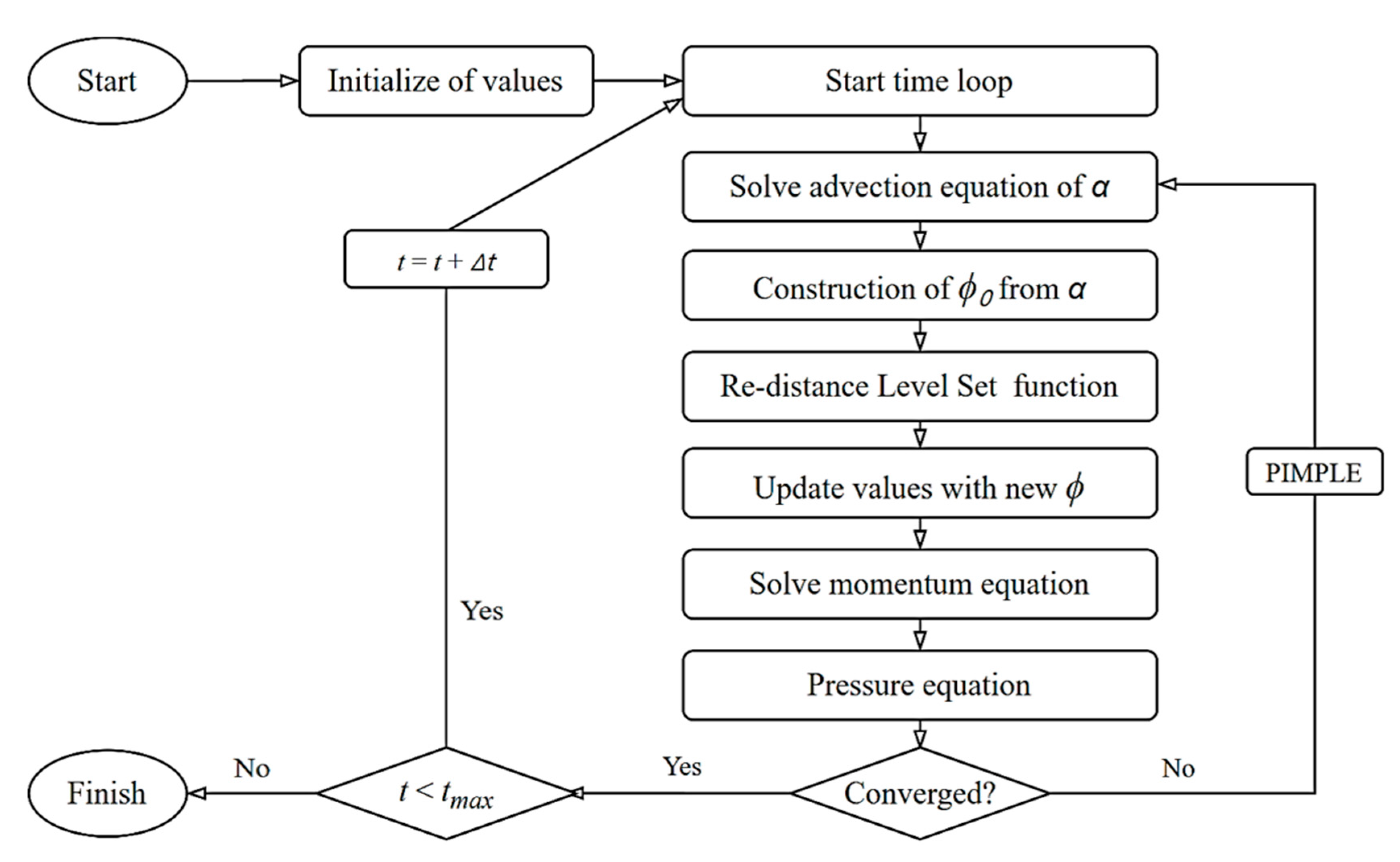
The flow chart of the CLSVOF method is shown in Figure 4. The flow chart and equations were based on Albadawi et al. [17]. In the CLSVOF method, the level-set method was started from the solution of the VOF method. The volume fraction ($\alpha$), which was the solution of the volume fraction transport equation, was used in the initial level-set function (${\varphi }_o$). The initial level-set function could be expressed as

$${\varphi }_0=\left(2\alpha -1\right)\Gamma$$

(6)

The volume fraction of 0.5 was defined as the initial interface in the level-set function because the isosurface of 0.5 is usually defined as the interface in the VOF method. The initial level-set function has a positive value in the air and a negative value in the water. The non-dimensional number ($\Gamma$) was defined using the cell size ($△x$) and defined as

$$\Gamma =0.75△x$$

(7)

The non-dimensional number was related to numerical stability and accuracy. A large non-dimensional number caused numerical instability, while a small nondimensional number caused an inaccurate result.

The level-set function was redistancing from the initial level-set function. The level-set function of each cell was calculated using the normal distance from the interface. The reinitialization equation could be expressed as

$$\frac{\partial \varphi }{\partial \tau }=Sign\left({\varphi }_0\right)\left(1-\left|\nabla \varphi \right|\right)$$

(8)

where $\tau$ is the artificial time step, and was selected as $\tau =0.1△x$.

The mixture density and dynamics viscosity were calculated using the Heaviside function ($H_{\varepsilon }\left(\varphi \right)$). The mixture density and dynamic viscosity were expressed as

$$H_{\varepsilon }\left(\varphi \right)=\{\begin{array}{cc} 0& if \varphi <-\varepsilon \\ \frac{\varphi +\varepsilon }{2\varepsilon }+\frac{sin\left(\pi \varphi /\varepsilon \right)}{2\pi }& if \left|\varphi \right|\le \varepsilon \\ 1& if \varphi >\varepsilon \end{array}$$

(9)

$${\rho }_{i,j}=H_{\varepsilon }\left(\varphi \right){\rho }_1+\left(1-H_{\varepsilon }\left(\varphi \right)\right){\rho }_2$$

(10)

$${\mu }_{i,j}=H_{\varepsilon }\left(\varphi \right){\mu }_1+\left(1-H_{\varepsilon }\left(\varphi \right)\right){\mu }_2$$

(11)

where $\epsilon$ is the interface thickness. The Heaviside function has values of zero and one outside the interface thickness ($\left|\varphi \right|\le \varepsilon$), and smoothly connects zero and one within the interface thickness. The interface thickness was chosen as $\epsilon =1.5∆x$. The continuum surface force in the level-set function could be expressed as [16]

$$F_{\sigma ,\varphi }=\sigma k_{\varphi }{\delta }_{\varphi }\nabla \varphi$$

(12)

where $\sigma$ is the surface tension coefficient, and ${\delta }_{\varphi }$ is the Dirac function, which is to activate the surface tension within the interface. The Dirac function and interface curvature could be written as

$${\delta }_{\varphi }\{\begin{array}{c}\begin{array}{cc}\frac{1}{2\varepsilon }\left(1+cos\left(\frac{\pi \varphi }{\varepsilon }\right)\right)& \left|\varphi \right|\le \varepsilon \\ 0& \left|\varphi \right|>\varepsilon \end{array}\end{array}$$

(13)

$$\kappa \left(\varphi \right)=-\nabla ·\frac{\nabla \varphi }{\left|\nabla \varphi \right|}$$

(14)

3.2.3. Verification of CLSVOF

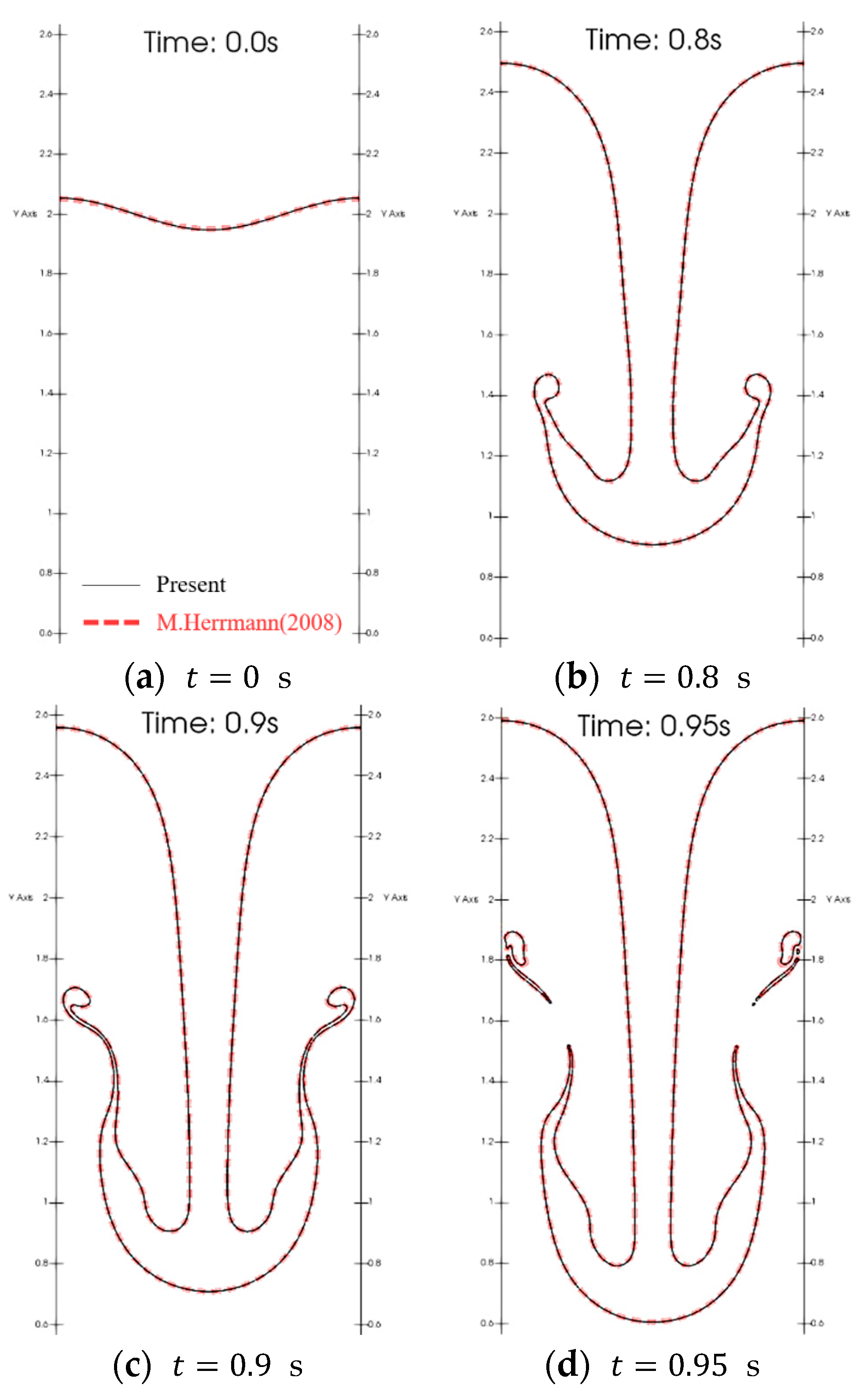
The Rayleigh–Taylor instability, which was used to verify complex multiphase flows, has been used by many researchers to compare their numerical methods. This is a mixing problem in which a dense fluid mixes with a low-density fluid, and is used to study the accuracy of reproducing the instability of the interface. Two fluids with different densities (${\rho }_1=1.225\frac{kg}{m^3}$, ${\rho }_2=0.1694\frac{ kg}{m^3}$) but the same viscosity (${\mu }_{1 }=0.00313\frac{kg}{m·s}, {\mu }_{2 }=0.00313 \frac{kg}{m·s}$) were selected. The domain extent was $1 \mathrm{m} \times 4 \mathrm{m}$ and the initial interface was set by the Cosine function, which was the wavelength of $1 \mathrm{m}$ and amplitude of $0.05 \mathrm{m}$. Gravity ($g$) was $9.81 \mathrm{m}/{\mathrm{s}}^2$ and the time step size ($△t$) was set to $2.5\times {10}^{-4} \mathrm{s}$. The grid size ($h_G$) was 1/256. The two-dimensional analysis was carried out for the Rayleigh–Taylor instability. Figure 5 shows the interface shapes at 0 s., 0.8 s., 0.9 s, and 0.95 s. and compares with another numerical result [23]. Both the stem shape and bubble shape were well simulated.

3.3. Numerical Methods

The time derivative terms were discretized using the Crank–Nicholson implicit scheme. The gradient at the cell centers was calculated using the least-squares method. The convection terms were discretized using a second-order accurate total variation diminishing (TVD) scheme with the Gauss van Leer limiter [24]. The velocity and pressure coupling and overall solution procedure were based on the PIMPLE algorithm. The PIMPLE Algorithm is a combination of PISO (Pressure Implicit with Splitting of Operator) and SIMPLE (Semi-Implicit Method for Pressure-Linked Equations) algorithm. The discretized algebraic equations for pressure and velocity were solved using a pointwise Gauss–Seidel iterative algorithm, while an algebraic multigrid method was employed to accelerate solution convergence [25].

The time step was set to $1\times {10}^{-3} \mathrm{s}$. The simulation time was advanced when the normalized residuals for the solutions had dropped by seven orders of magnitude.

4. Results and Discussion

4.1. Domain Extents, Boundary Conditions, and Meshes

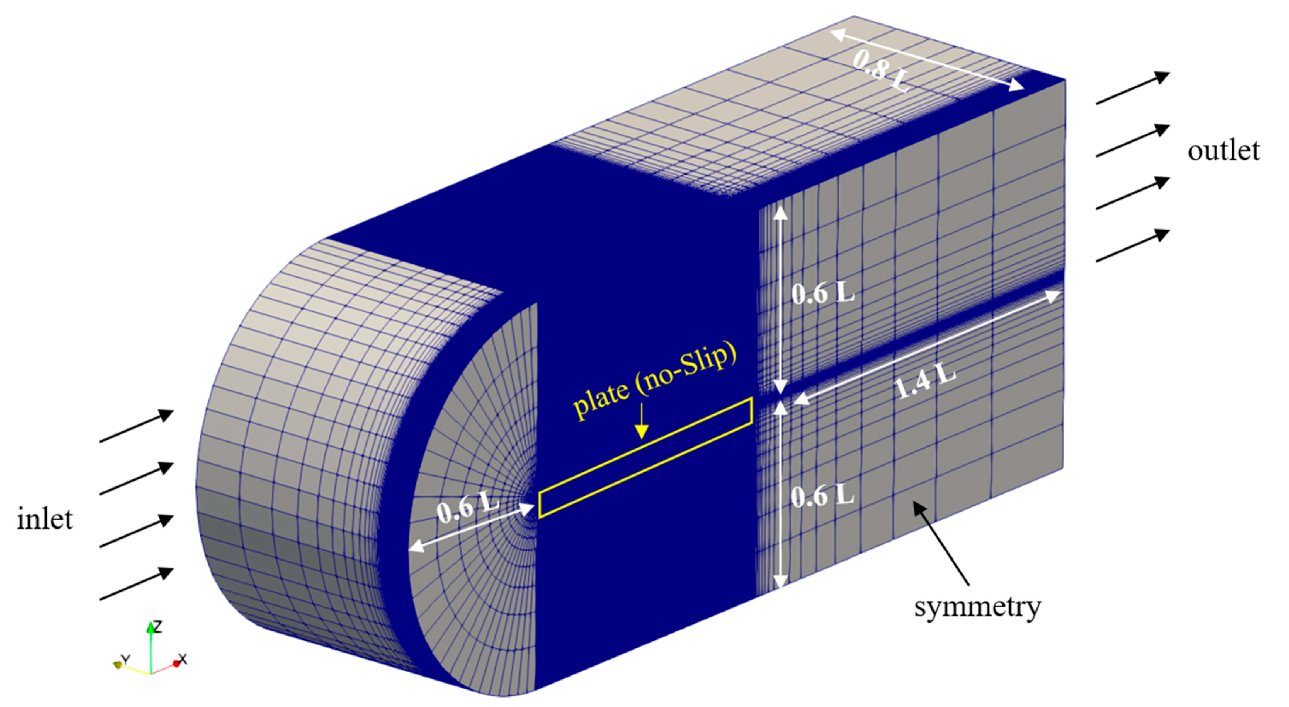
The stern direction of the flat plate was set as the + x-axis, the starboard direction as the + y-axis, and the height direction as the + z-axis. The domain extent was set to 0.6 L in the forward direction, 1.4 L in the stern direction, 0.8 L in the width direction, and 0.6 L above and below the flat plate. Here, L is the length of the flat plate. The air was injected from the bottom in the—z-direction. Figure 6 shows the domain extent, boundary conditions, and meshes.

The Dirichlet conditions were applied for the velocity, turbulence, and volume fraction at the inlet boundary and the pressure at the outlet boundary. The Neumann conditions were applied for the pressure at the inlet boundary, and the velocity, turbulence, and volume fraction at the outlet boundary [26]. Only half of the flat plate was considered because the shape was symmetrical. The symmetry condition was applied to the plane of y = 0.

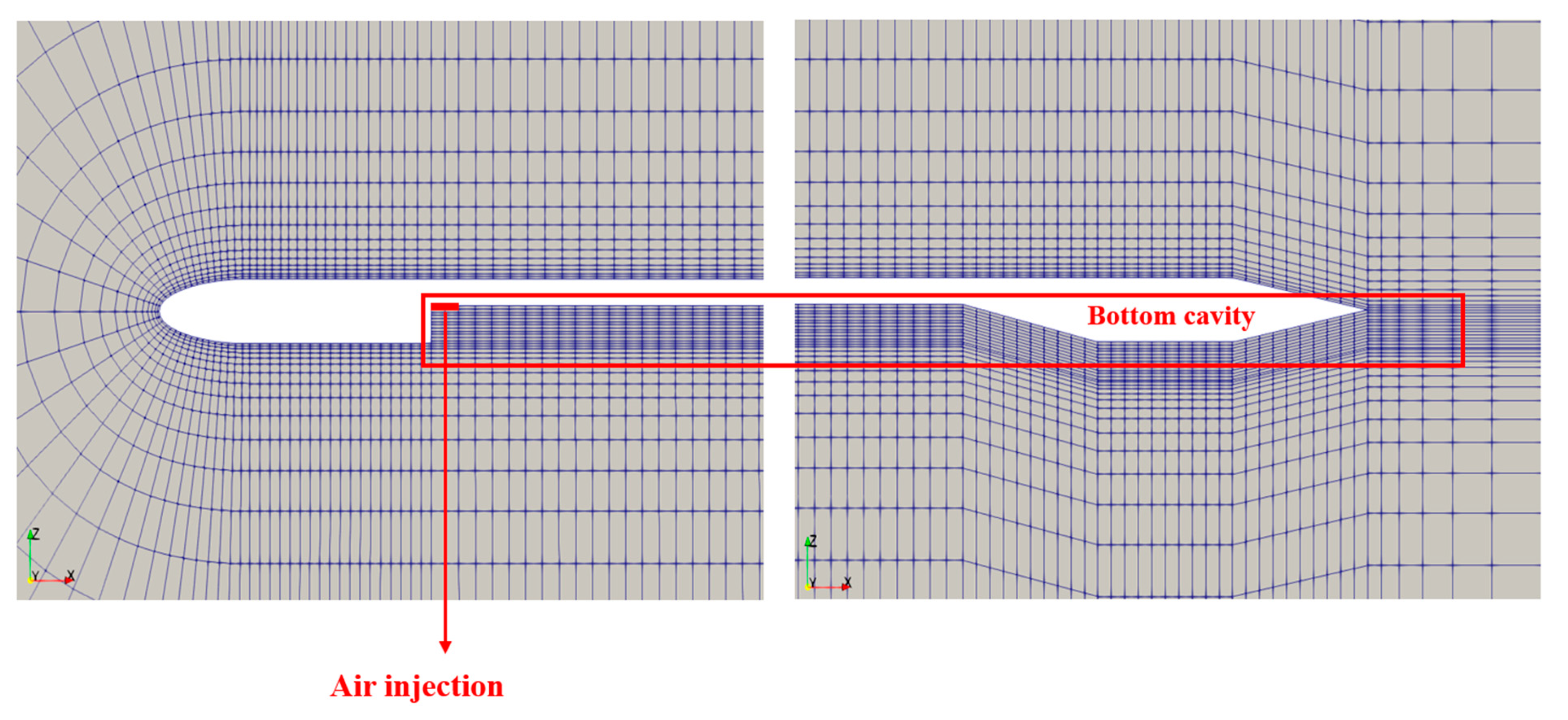
Figure 7 shows typical internal meshes at the y = 0 plane. For an accurate prediction of the air layer in the bottom air cavity, structured meshes were used.

4.2. Grid Uncertainty Assessment

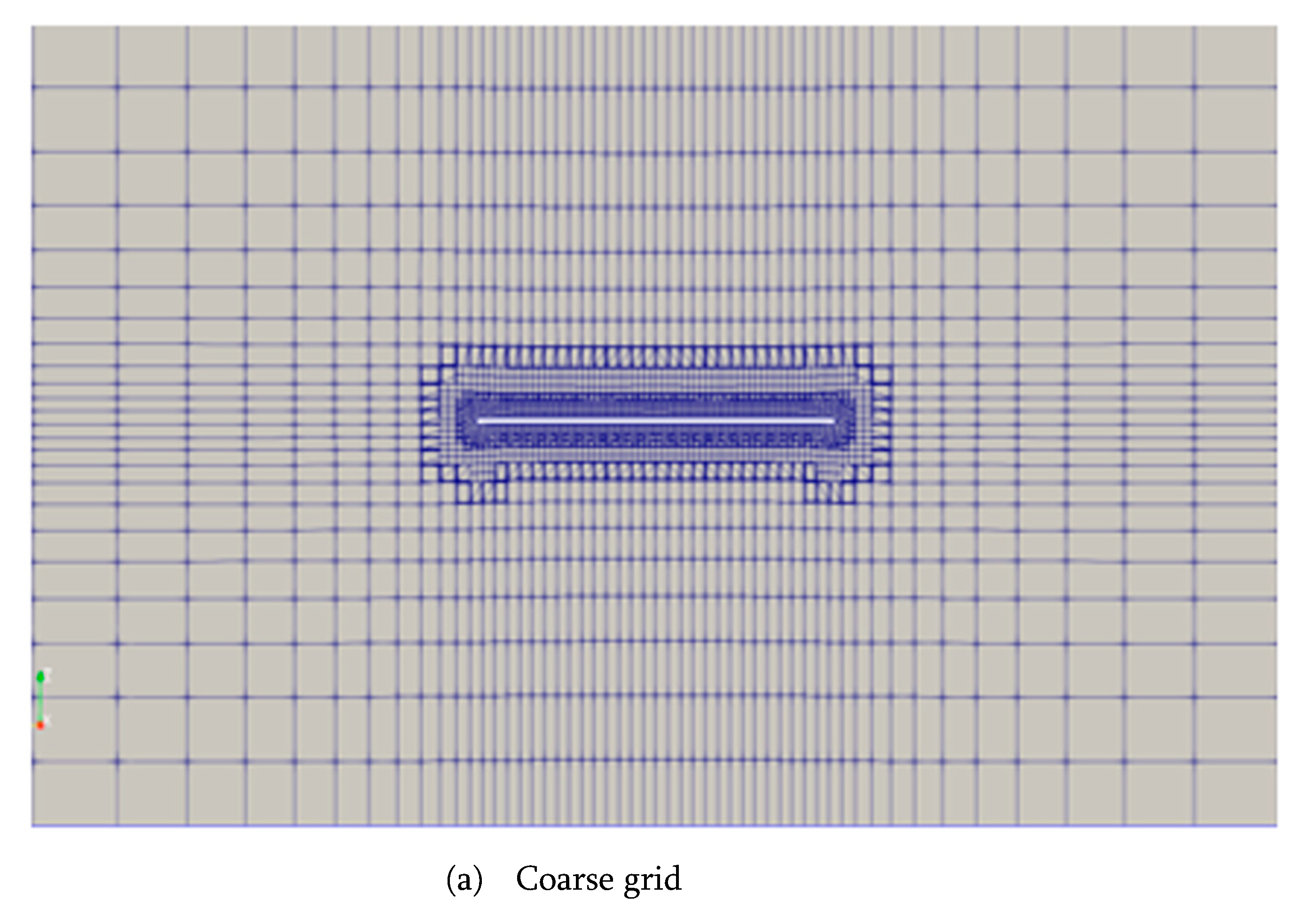
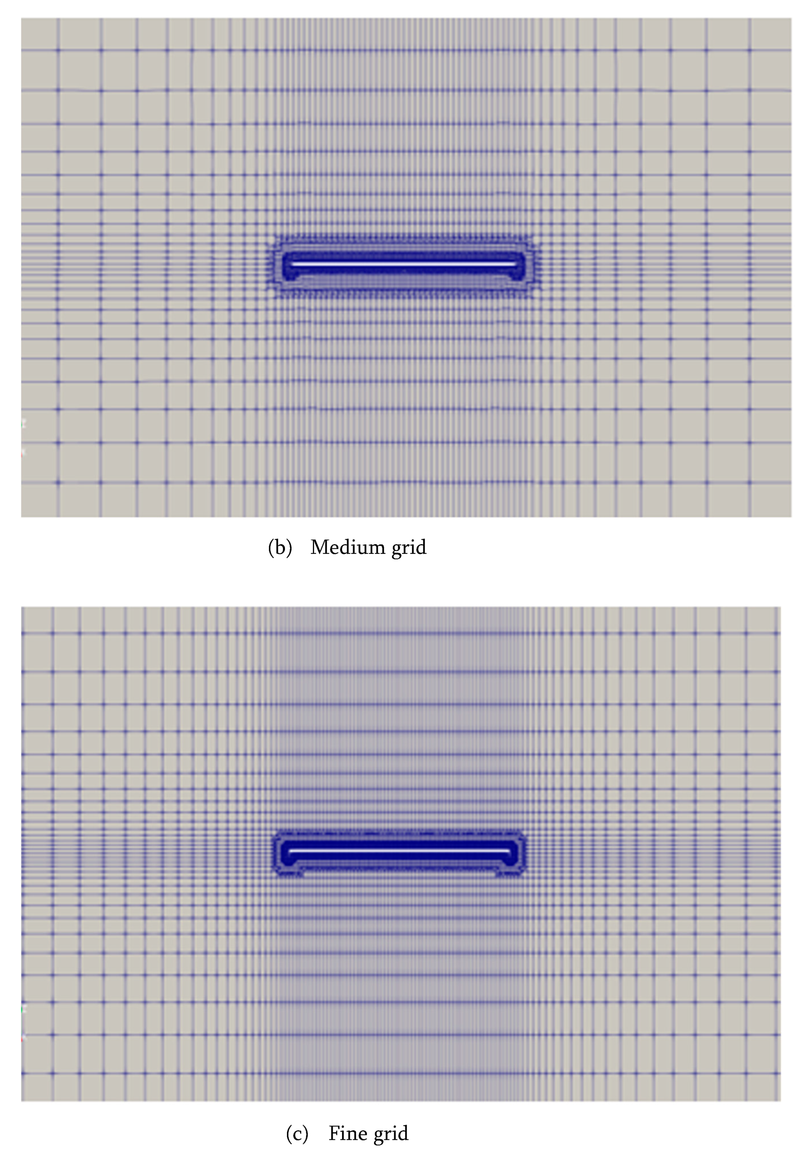
Grid uncertainty for the total drag reduction and covered area of the injected air were assessed with three types of grids. As listed in

Table 2. Grid number for uncertainty assessment.

Grid System	Background Grid Size (m)	Grid Count
Coarse	0.06	1,245,645
Medium	0.042	2,822,109
Fine	0.03	4,778,028

, three types of grid, i.e., coarse, medium, and fine grids, were considered. Figure 8 shows the typical internal meshes at the y-z plane. The background structured grid size was increased or decreased in all directions by 1.4 times each. The finally considered total grid counts were $1.2\times {10}^6$ for the coarse grid, $2.8\times {10}^6$ for the medium grid, and $4.8\times {10}^6$ for the fine grid.

Table 3. Results of grid convergence test.

Parameter	${\mathit{\eta }}_{\mathit{T}}$	${\mathit{\zeta }}_{\mathit{a}\mathit{i}\mathit{r}}$
Fine ($S_{G, 1}$)	0.312	0.999
Medium ($S_{G, 2}$)	0.311	0.997
Coarse ($S_{G, 3}$)	0.308	0.989
$R_G$	0.333	0.25
${\delta }_G{}^{*}\left(\% S_{G, 1}\right)$	−0.001 (−0.32%)	−0.002 (−0.20%)
$U_G{}^{*}\left(\% S_{G, 1}\right)$	0.0015 (0.48%)	0.00333 (0.33%)
$U_{GC}{}^{*}\left(\% S_{G, 1}\right)$	0.0005 (0.16%)	0.00133 (0.13%)

lists the results of the grid uncertainty assessment for the total drag reduction (${\eta }_T$) and coverage area of the injected air (${\zeta }_{air}$). The convergence ratios ($R_G=\frac{S_{G,2} - S_{G,1}}{S_{G,3} - S_{G,2}}$) showed a monotonic convergence ($0 <R_G < 1$). Using the correction factor ($C$), the corrected error (${\delta }_G{}^{*}$), uncertainty ($U_G$), and corrected uncertainty ($U_{GC})$ were calculated as

$$C=\frac{r_G{}^{p_i} - 1}{r_G{}^{p_{est}} - 1}.$$

(15)

$${\delta }_G{}^{*}=C{\delta }_{R{E}_G}{}^{*}=C\left(\frac{{\epsilon }_{G,21}}{r_i{}^{p_i}-1}\right).$$

(16)

$$U_G=|C{\delta }_{R{E}_G}{}^{*}|+|\left(1-C\right){\delta }_{R{E}_G}{}^{*}.$$

(17)

$$U_{GC}=\left|\left(1-C\right){\delta }_{R{E}_G}{}^{*}\right|$$

(18)

The grid uncertainty and corrected grid uncertainty for the total drag reduction were 0.48% and 0.16%, respectively. The grid uncertainty and corrected grid uncertainty for the coverage area of the injected air were 0.33% and 0.13%, respectively. The level of verification and validation was less than 1%.

4.3. Air Lubrication Method and Drag Reduction

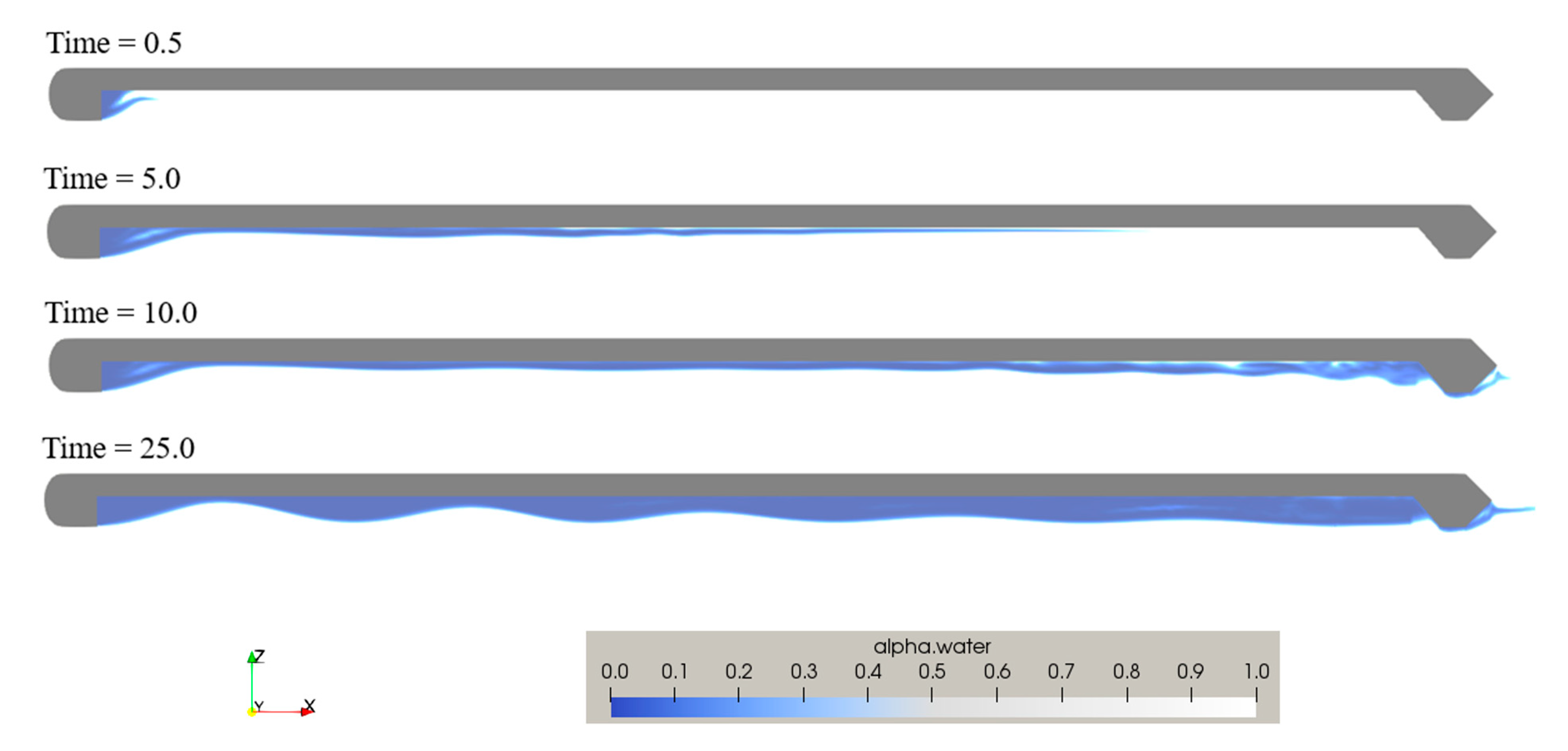
The computations were carried out at a Froude number of 0.173 and the injected airflow rate of 0.149 ${\mathrm{m}}^3/\mathrm{s}$. Figure 9 shows the streamlines around the flat plate and inside the bottom air cavity. The flow was circulated in the fore region of the bottom air cavity, which was similar to the flow of the backward-facing step. Figure 10 shows the air layer evolution in the bottom air cavity. The injected air filled the circulation zone and then convected downstream. After the injected air filled the bottom surface, the air layer thickness was increased.

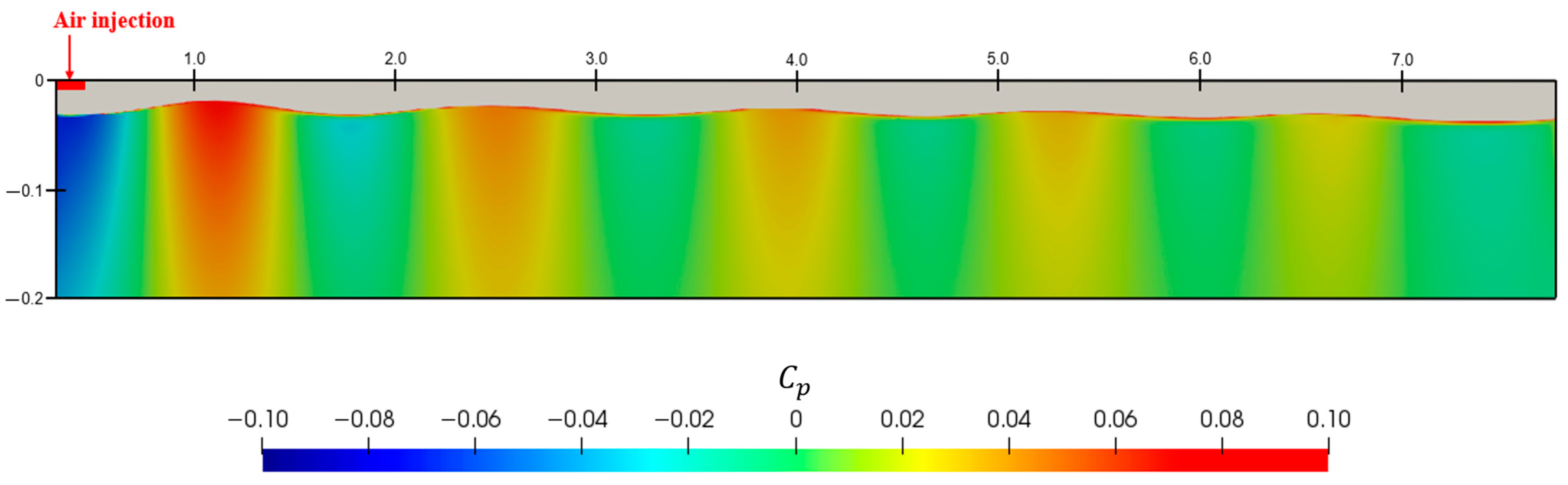
The air circulation zone causes low pressure outside the air layer, as shown in Figure 11. The repeated high and low pressures outside the air layer caused an undulation of the air layer, which generated an air layer wave. The generated air layer wave is observed in Figure 11. The air layer wave was related to the velocity of the injected air, and can be expressed with the equation below [27].

$$\lambda =\frac{2\pi U^2}{g}$$

(19)

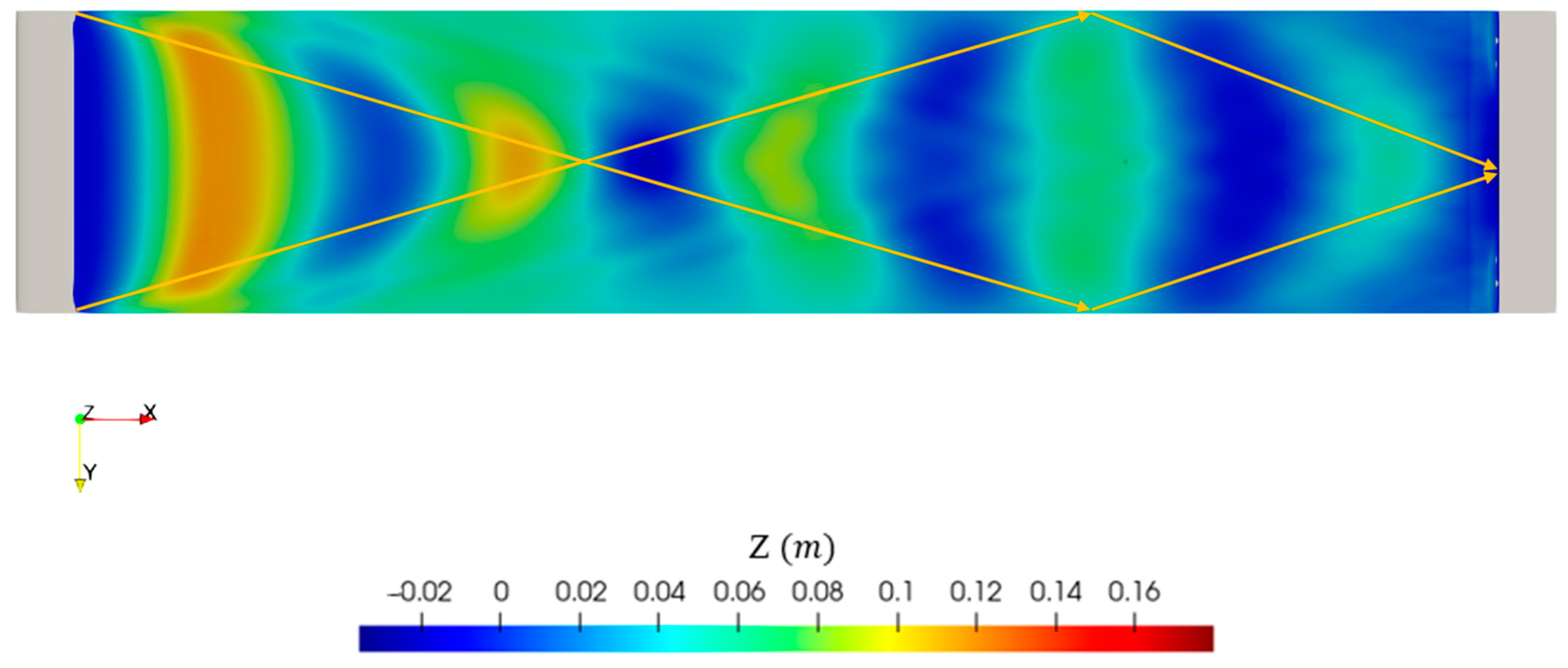
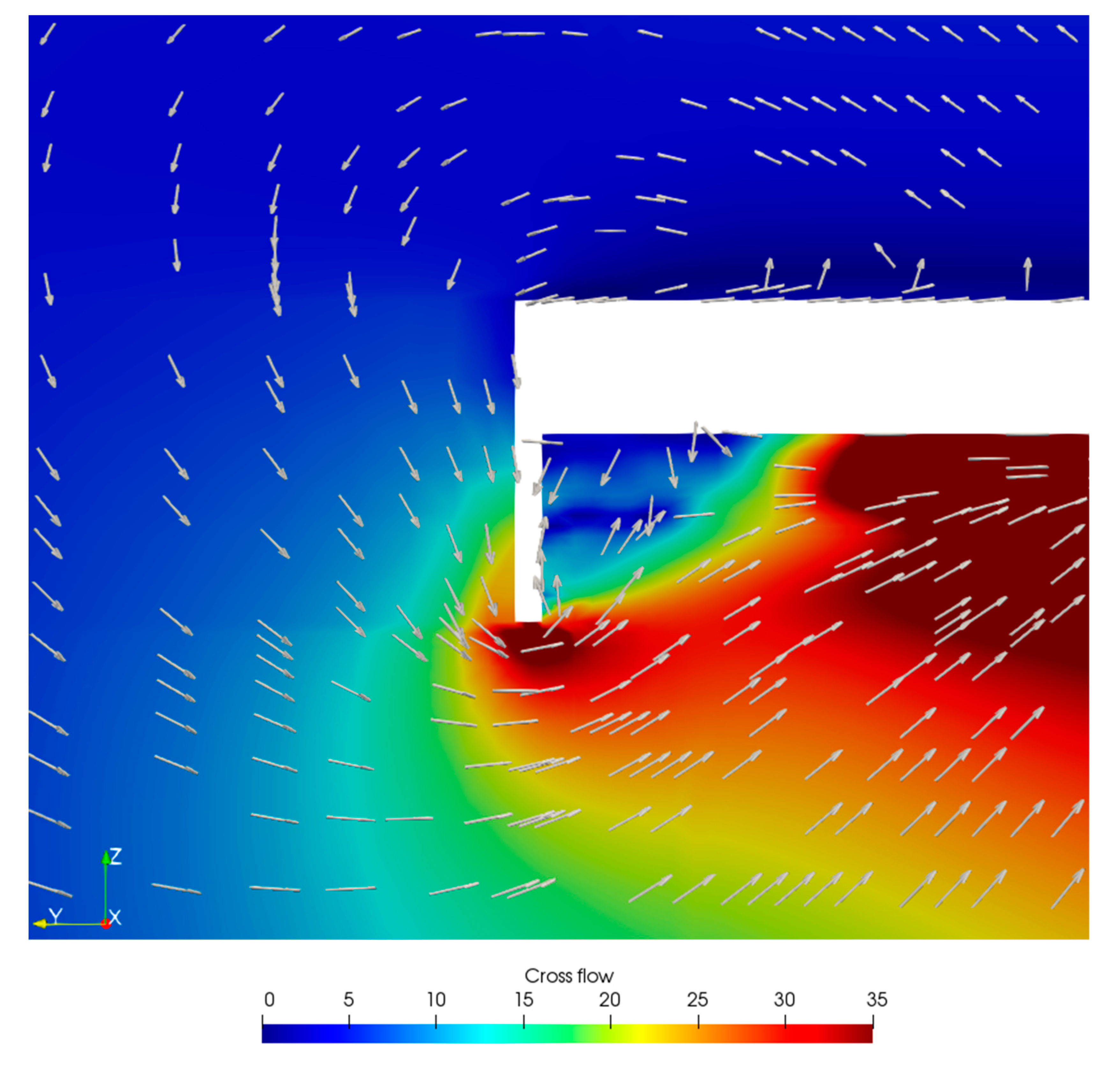
The calculated wavelength of the air layer was $\lambda =\frac{2\pi U^2}{g}=1.5$, which was similar to the result in Figure 11. This equation was of the same form as the phase velocity in the airy wave theory. The propagation characteristic of the air layer was similar to the ocean wave. Figure 12 shows the air layer elevation. The five air layer waves were seen in the bottom air cavity. Note that the air layer showed converging and diverging flow patterns. Figure 13 shows the crossflow ($\sqrt{u_y^2+u_z^2}$) at the flat plate at x = 0.5 m. The cross-flow was generated because of the different pressures at the side thin plate of the bottom air cavity. This cross-flow caused the diverging of the air layer around the fore region in the bottom air cavity. Diverging and converging flow patterns were then observed.

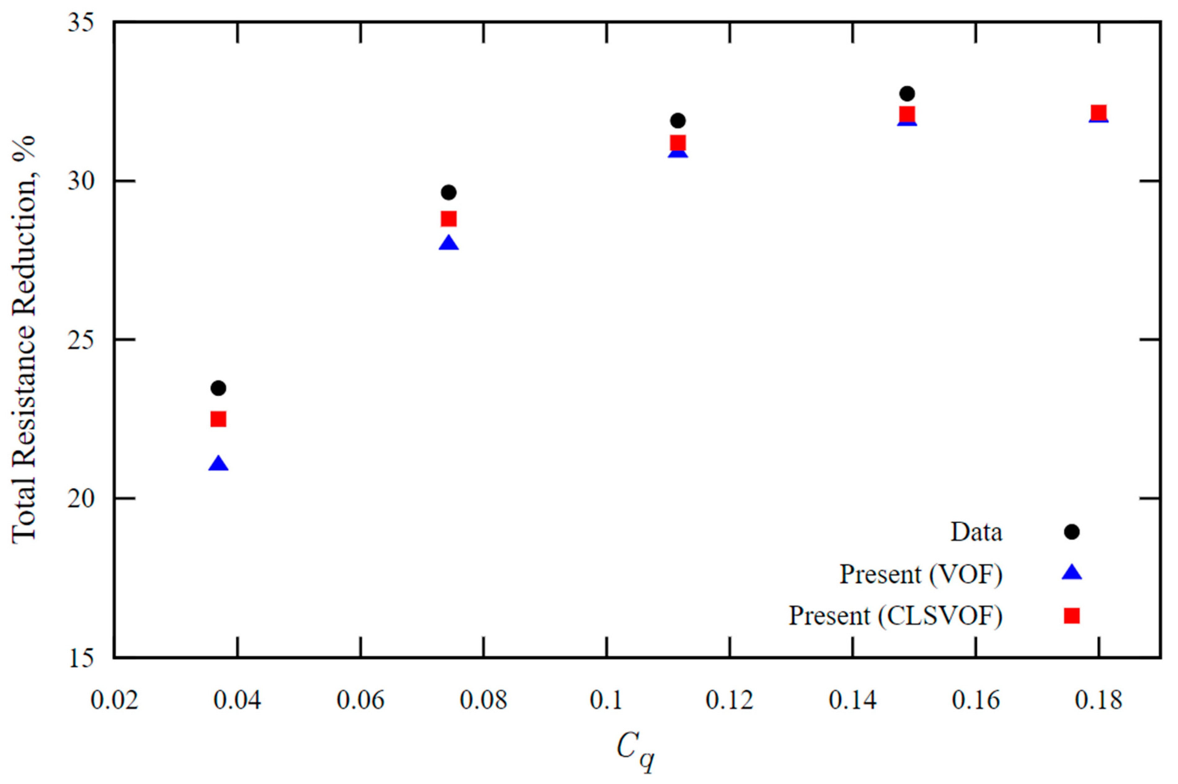
The drag reduction of the flat plate was predicted using the CLSVOF and VOF solvers. Figure 14 shows the total drag reduction rate (${\eta }_T$) for various injected airflow rates ($C_q$). It could be observed that the total drag reductions were constant when the injected airflow rates were greater than 0.14, because the frictional drag by the air lubrication did not decrease further. After the air layer completely covered the surface of the bottom cavity, no additional frictional drag reduction could be obtained. At high injected airflow rates, the total drag reductions shown by both the VOF and CLSVOF solvers were similar to those by the experimental results [12]. Similar reductions were obtained using both solvers because the air layer covered the whole bottom cavity. On the other hand, at low injected airflow rates, the air layer showed a shape of BDR or TALDR, so it could be seen that the CLSVOF solver was more similar to the experimental data than the VOF solver.

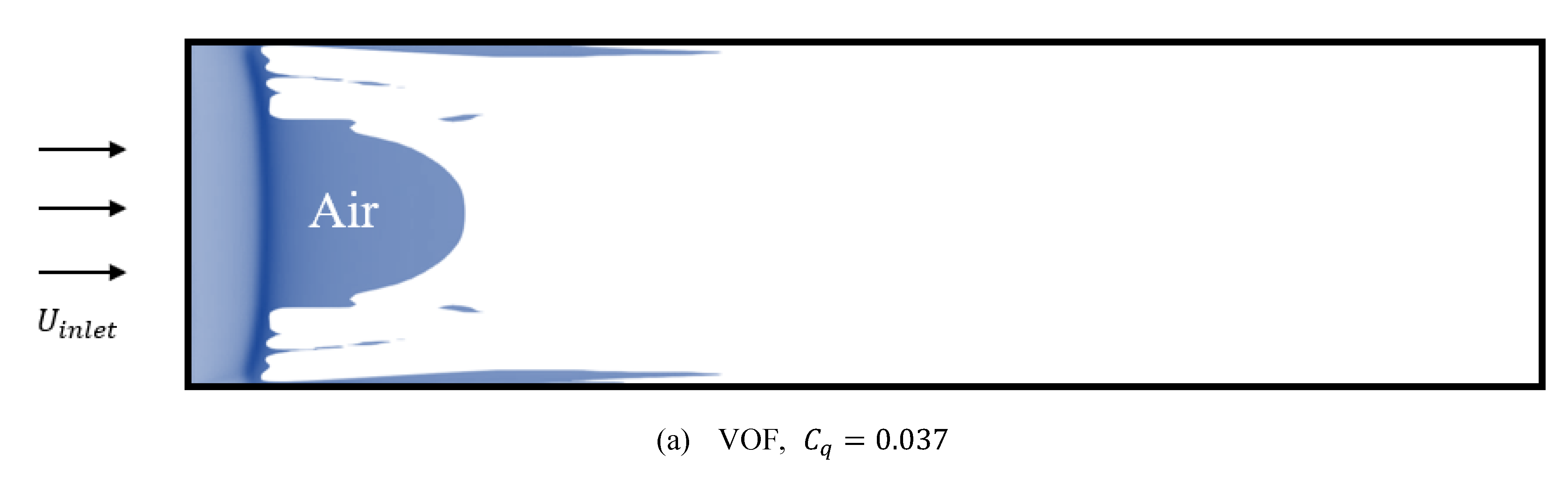
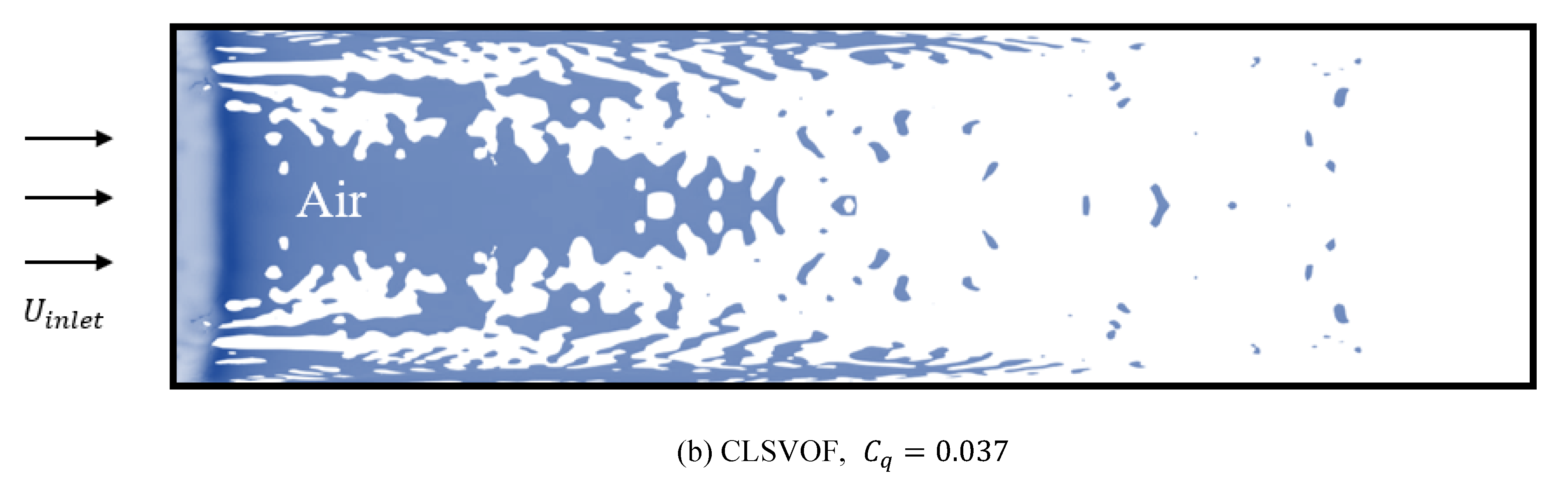
The air layer shape for both the CLSVOF and VOF solvers were compared. Figure 15 shows the air layer at the low injected airflow rate of 0.037. In the CLSVOF solver, the air layer was discontinuously observed over a large area, but only a continuous air layer was observed in the VOF solver. It was confirmed that the shape of the air layer by the VOF solver caused a decrease in the total drag reduction. Figure 16 shows the air layer at the high injected airflow rate of 0.18. The air layer was continuously distributed by both the solvers. The air layer shapes were similar in the ALDR regime, indicating that the VOF solver was limited in terms of its capacity to predict the discontinuous air layer.

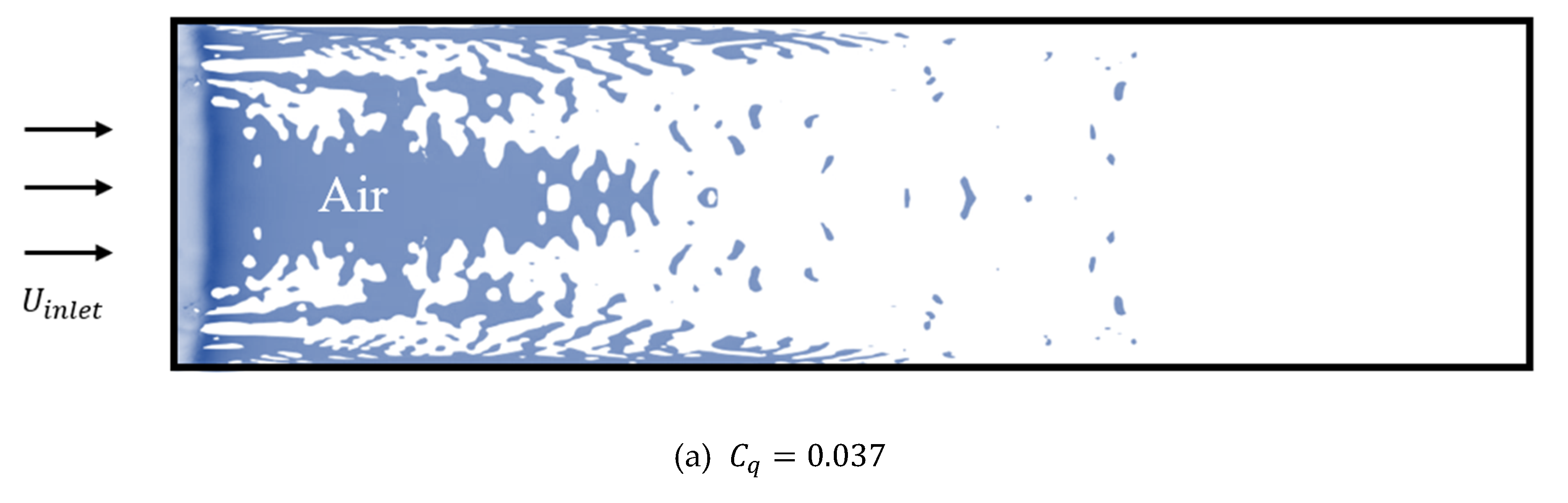
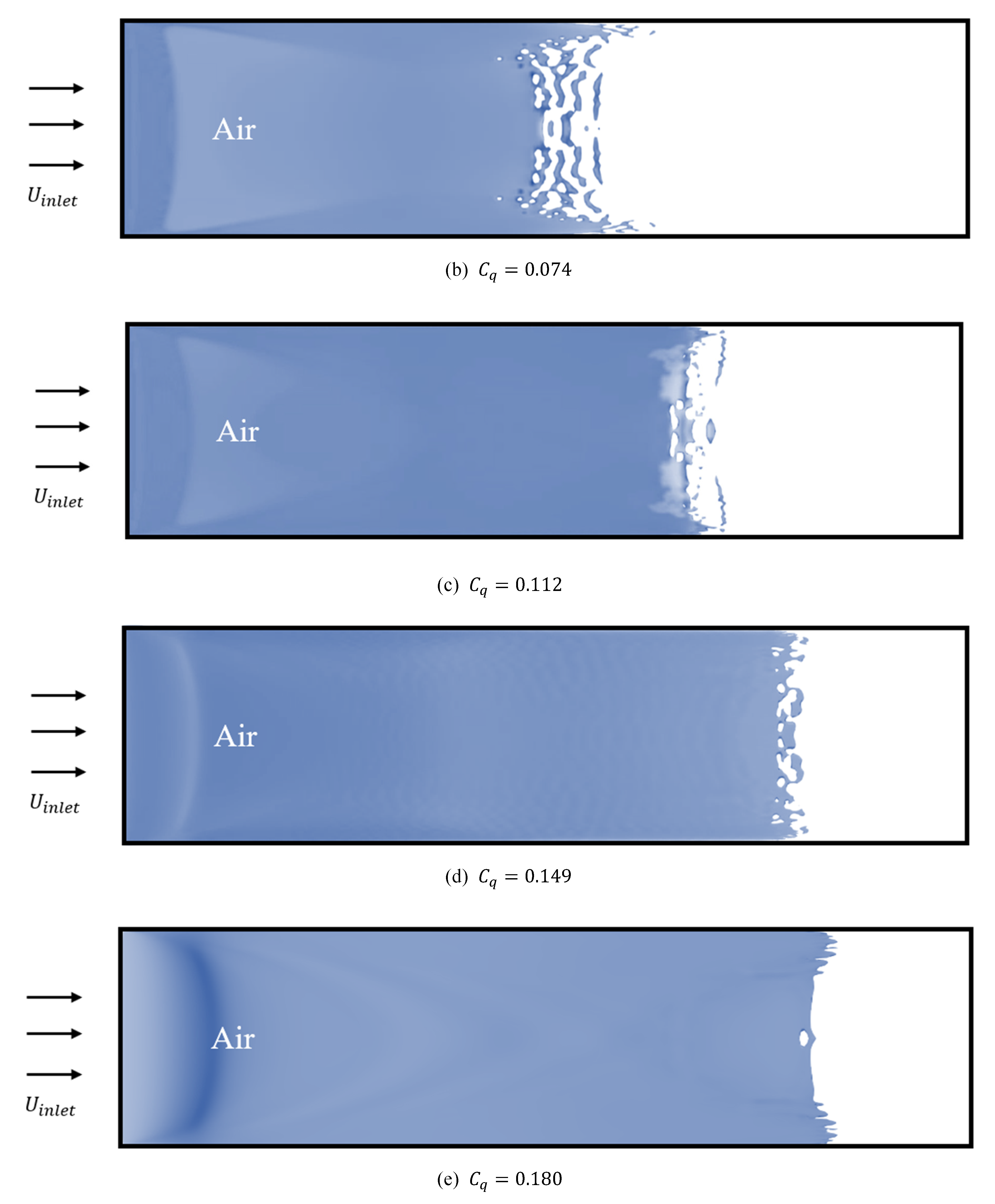
Figure 17 shows the air layer for various injected airflow rates according to the CLSVOF solver. At the low injected airflow rate of 0.037, bubbles appeared discontinuously. As the injected airflow rate increased, the continuous air layer was widened, and at the end of the air layer, a discontinuous air layer was observed. The time required for the air layer to evolute to its maximum length was calculated as 16.9 s, 10.2 s, 8.8 s, 8.1 s, and 7.9 s when the airflow rates were 0.037, 0.074, 0.112, 0.149, and 0.180, respectively. As the injected airflow rate increased, the air layer evolution speed increased.

Table 4. Drag and drag reduction.

	Present (CLSVOF)	Experiment (Hao et al. [12])	Difference
$R_T$	$41.9 \mathrm{N}$	$41.8 \mathrm{N}$	$0.24\%$
$R_v$	$28.3 \mathrm{N}$	$28.1 \mathrm{N}$	$0.71\%$
${\eta }_T$	$32.1\%$	$33\%$	$-0.9\%$
${\eta }_f$	$32.3\%$	$31.5\%$	$0.8\%$

lists the results with a Froude number of 0.173 and the injected airflow rate of 0.149. Here $R_T$ is the total drag of the flat plate, $R_v$ is the frictional drag, ${\eta }_T$ is the total drag reduction, and ${\eta }_f$ is the frictional drag reduction. It can be seen that the CLSVOF solver predicted the drag reduction in the air lubrication method well.

5. Concluding Remarks

In the present study, the CLSVOF solver was selected to simulate air lubrication of a flat plate. The CLSVOF solver was developed using OpenFOAM, an open-source computational fluid dynamics platform. The air layer shape and drag reduction achieved by the air lubrication were observed for various injected airflow rates.

The recirculating flow inside the bottom cavity appeared like a backward-facing step. The air layer showed an undulation and the fluctuating period of the air layer was similar to the ocean wave. The cross-flow at the side edge of the flat plate caused a converging and diverging flow pattern of the air layer.

As the injected airflow rate increased, the air layer developed from the BDR to ALDR regimes. After the air layer covered the whole surface, the frictional drag did not decrease even if the airflow rate increased, so that the total drag was constant. When the air layers simulated by both the CLSVOF and VOF solvers were compared, it was found that the VOF solver had limitations in terms of reproducing a discontinuous air layer. It was confirmed that CLSVOF was needed to predict the air layer well in air lubrication systems. The CLSVOF solver is planned to be used to predict the drag of a ship with the air lubrication system in the model and full scales.

References

- Nobuaki, S.; Hiroshi, K.; Kunihide, O.; Yasutaka, K.; Björn, W.; Hikaru, K. An overset RaNS prediction and validation of full scale stern wake for 1600TEU container ship and 63,000 DWT bulk carrier with an energy saving device. Appl. Ocean Res. 2020, 105, 102–417. [Google Scholar]
- Park, S.; Oh, G.; Rhee, S.H.; Koo, B.-Y.; Lee, H. Full scale wake prediction of an energy saving device by using computational fluid dynamics. Ocean Eng. 2015, 101, 254–263. [Google Scholar] [CrossRef]
- Zeynep, T.; Noriyuki, S.; Mehmet, A.; Emin, K. An investigation into effects of Gate Rudder system on ship performance as a novel energy-saving and manoeuvring device. Ocean Eng. 2020, 218, 108–250. [Google Scholar]
- Walsh, M. Turbulent Boundary Layer Drag Reduction using Riblets. In Proceedings of the 20th Aerospace Science Meeting, Orlando, FL, USA, 11–14 January 1982. [Google Scholar]
- Gray, J. Studies in Animal Locomotion VI. The Propulsive Powers of the Dolphin. J. Exp. Biol. 1936, 13, 192–199. [Google Scholar]
- Lee, J.; Kim, S.; Kim, B.; Jang, J.; McStay, P. Full scale applications of air lubrication for reduction of ship frictional resistance. In Proceedings of the SNAME Maritime Convention 2017, Houston, TX, USA, 24–28 October 2017. [Google Scholar]
- Mizokami, S.; Kawakita, C.; Kodan, Y. Experimental Study of Air Lubrication Method and Verification of Effects on Actual Hull by Means of Sea Trial. Mitsubishi Heavy Ind. Tech. Rev. 2010, 47, 41–47. [Google Scholar]
- Mäkiharju, S.A.; Marc, P.; Steven, L.C. On the energy economics of air lubrication drag reduction. Int. J. Nav. Arch. 2012, 4, 412–422. [Google Scholar] [CrossRef] [Green Version]
- Du, P.; Wen, J.; Zhang, Z.; Song, D.; Ouahsine, A.; Hu, H. Maintenance of air layer and drag reduction on superhydrophobic surface. Ocean Eng. 2017, 130, 328–335. [Google Scholar] [CrossRef]
- Mäkiharju, S.; Lee, I.; Filip, G. The topology of gas jets injected beneath a surface and subject to liquid cross-flow. J. Fluid Mech. 2017, 818, 141–183. [Google Scholar] [CrossRef]
- Park, S.H.; Lee, I. Optimization of drag reduction effect of air lubrication for a tanker model. Int. J. Naval Arch. Ocean Eng. 2018, 10, 427–438. [Google Scholar] [CrossRef]
- Hao, W.U.; Yongpeng, O.U.; Qing, Y.E. Experimental study of air layer drag reduction on a flat plate and bottom hull of a ship with cavity. Ocean Eng. 2019, 183, 236–248. [Google Scholar] [CrossRef]
- Kim, S.-Y.; Ha, J.-Y.; Paik, K.-J. Numerical study on the extrapolation method for predicting the full-scale resistance of a ship with an air lubrication system. J. Ocean Eng. Technol. 2020, 34, 387–393. [Google Scholar] [CrossRef]
- Kim, H.; Kim, H.; Lee, D. Study on the skin-frictional Drag Reduction Phenomenon by Air Layer using CFD Technique. J. Soc. Naval Arch. Korea 2019, 56, 361–371. [Google Scholar] [CrossRef]
- Bourlioux, A. A coupled level-set volume-of-fluid algorithm for tracking material interfaces. In Proceedings of the 6th International Symposium on Computational Fluid Dynamics, Lake Tahoe, NV, USA, 4–8 September 1995; pp. 15–22. [Google Scholar]
- Brackbill, J.; Kothe, D.; Zemach, C. A continuum method for modeling surface tension. J. Comput. Phys. 1992, 100, 335–354. [Google Scholar] [CrossRef]
- Albadawi, A.; Donoghue, D.B.; Robinson, A.J.; Murray, D.B.; Delauré, Y.M.C. Influence of surface tension implementation in Volume of Fluid and coupled Volume of Fluid with Level Methods for bubble growth and detachment. Int. J. Multiph. Flow 2013, 53, 11–28. [Google Scholar] [CrossRef]
- Dianat, M.; Skarysz, A.; Garmory, A. A coupled level set and volume of fluid method for automotive exterior water management applications. Int. J. Multiph. Flow 2017, 91, 19–38. [Google Scholar] [CrossRef] [Green Version]
- Li, Q.; Ouyang, J.; Yang, B.; Li, X. Numerical simulation of gas-assisted injection molding using CLSVOF method. Appl. Math. Model. 2012, 36, 2262–2274. [Google Scholar] [CrossRef]
- Menter, F. Two Equation Eddy-Viscosity Turbulence Modeling for Engineering Applications. AIAA J. 1994, 32, 1598–1605. [Google Scholar] [CrossRef] [Green Version]
- Hirt, C.W.; Nichols, B.D. Volume of fluid (VOF) method for the dynamics of free boundaries. J. Comput. Phys. 1981, 39, 201–225. [Google Scholar] [CrossRef]
- Park, S. Development of free-surface decomposition method and its application. J. Adv. Res. Ocean Eng. 2017, 3, 75–82. [Google Scholar]
- Herrmann, M. A balanced force refined level set grid method for two-phase flows on unstructured flow solver grids. J. Comput. Phys. 2008, 227, 2674–2706. [Google Scholar] [CrossRef]
- Park, S.; Seok, W.C.; Park, S.T.; Rhee, S.H.; Choe, Y.; Kim, C.; Kim, J.H.; Ahn, B.K. Compressibility effects on cavity dynamics behind a two-dimensional wedge. J. Mar. Sci. Eng. 2020, 8, 39. [Google Scholar] [CrossRef] [Green Version]
- Weiss, J.; Maruszewski, J.; Smith, W. Implicit Solution of Preconditioned Navier–tokes Equations Using Algebraic Multigrid. AIAA J. 1999, 37, 29–36. [Google Scholar] [CrossRef]
- Song, S.; Park, S. Unresolved CFD and DEM coupled solver for particle-laden flow and its application to single particle settlement. J. Mar. Sci. Eng. 2020, 8, 983. [Google Scholar] [CrossRef]
- Shiri, A.; Anderson, M.; Bensow, R. Hydrodynamics of a Displacement Air Cavity Ship. In Proceedings of the 29th Symposium on Naval Hydrodynamics, Gothenburg, Sweden, 26–31 August 2012. [Google Scholar]
Figure 1.
Three shapes of air layer. Reprinted from Ref. [8].