Article

Study of the Sound Escape with the Use of an Air Bubble Curtain in Offshore Pile Driving

by
Yaxi Peng
1,*,
Apostolos Tsouvalas
1,2,
Tasos Stampoultzoglou
3 and
Andrei Metrikine
1,2
1
Section of Dynamics of Solids and Structures, Department of Structural Engineering, Delft University of Technology, Stevinweg 1, 2628 CN Delft, The Netherlands
2
Section of Offshore Engineering, Department of Hydraulic Engineering, Delft University of Technology, Stevinweg 1, 2628 CN Delft, The Netherlands
3
Department of Engineering & Estimating Offshore/Offshore Wind, Van Oord, Schaardijk 211, 3063 NH Rotterdam, The Netherlands
*
Author to whom correspondence should be addressed.
J. Mar. Sci. Eng. 2021, 9(2), 232; https://0-doi-org.brum.beds.ac.uk/10.3390/jmse9020232
Submission received: 31 January 2021 / Revised: 12 February 2021 / Accepted: 17 February 2021 / Published: 22 February 2021
(This article belongs to the Special Issue Offshore Wind Soil–Structure Interaction (SSI))

Abstract

:
Underwater noise pollution generated by offshore pile driving has raised serious concerns over the ecological impact on marine life. To comply with the strict governmental regulations on the threshold levels of underwater noise, bubble curtains are usually applied in practice. This paper examines the effectiveness of an air bubble curtain system in noise reduction for offshore pile driving. The focus is placed on the evaluation of noise transmission paths, which are essential for the effective blockage of sound propagation. A coupled two-step approach for the prediction of underwater noise is adopted, which allows us to treat the waterborne and soilborne noise transmission paths separately. The complete model consists of two modules: a noise prediction module for offshore pile driving aiming at the generation and propagation of the wave field and a noise reduction module for predicting the transmission loss in passing through an air bubble curtain. With the proposed model, underwater noise prognosis is examined in the following cases: (i) free-field noise prediction without the air bubble curtain, (ii) waterborne path fully blocked at the position of the air bubble curtain while the rest of the wave field is propagated at the target distance, (iii) similarly to (ii) but with a non-fully blocked waterborne path close to the seabed, and (iv) air bubble curtain modeled explicitly using an effective medium theory. The results provide a clear indication of the amount of energy that can be channeled through the seabed and through possible gaps in the water column adjacent to the seabed. The model allows for a large number of simulations and for a thorough parametric study of the noise escape when a bubble curtain is applied offshore.

1. Introduction

Anthropogenic impact on the marine environment caused by offshore pile driving has been intensified with the increasing deployment rate of offshore wind energy. The underwater noise generated from the construction of offshore wind farms poses a risk to the marine mammals and fish [1]. Their foraging behavior, migration, and communication are all correlated to the underwater sound, which can be disturbed severely due to the impulsive sound emitted in the course of pile driving [2,3]. To protect the marine ecosystem, many countries have imposed strict regulations on the threshold of sound pressure levels for offshore activities. Many noise mitigation systems (i.e., bubble curtains, hydro-sound damper, noise mitigation screen, etc.) have been developed over the last decade to prevent exceeding the threshold limits during pile installation [4]. Among them, air bubble curtain systems (ABC) are considered to be the most popular in use and have been applied in many projects over the last decade. The complete system is formed by rising air bubbles with the compressed air coming from a nozzle hose which encircles the pile. The presence of the bubble–seawater mixture characterized by relatively high compressibility causes a large impedance mismatch at the interface with the seawater which, in turn, causes incident acoustic waves to reflect in the domain between the pile and the air-bubble curtain. Secondary to wave reflection, the resonance of the air bubbles can also add to hydro-sound absorption. However, the resonance of typical small-size bubbles (i.e., 8 to 50 mm) takes effect solely at relatively high frequencies which lie outside the typical noise spectrum associated with pile driving of large-size monopiles (<400 Hz) [5].
To investigate the sound transmission in offshore pile driving, many noise prediction models have been developed over the last decade as discussed comprehensively by Tsouvalas [5]. Finite element (FE) [6] or finite difference [7] models are mostly used for the sound generation module in the near field. For the sound propagation in the far field, various techniques including the normal-mode method [8,9], the wavenumber integration method [10], or the parabolic equation (PE) method [6,11,12,13,14] have been applied in the past. In the models mentioned above, an equivalent fluid model is used to describe the sediment. Fricke and Rolfes [15] modeled the soil with the finite element method and the pile hammer with an analytical model. In contrast to numerical models, a semi-analytical model developed by Tsouvalas and Metrikine [16] uses the linear elastic thin shell theory to describe the pile dynamics, while the sediment is described by distributed springs and dashpots in all directions along the embedded part of the shell in the soil. The model mainly focus on the pile dynamics and near-field noise prediction. Motivated by the observation that the soil plays a significant role in noise transmission, a complete vibro-acoustic model capturing the interaction between the pile, water, and the soil was further developed in [17] with the seabed modeled as a layered linear elastic medium. A similar semi-analytical model, albeit with the fluidized description of the seabed, developed in [18,19] includes a non-axisymmetric force and an anvil, which shows the circumferential dependence of radiated pressure field and the pile–anvil interaction. Wilkes and Gavrilov [9] use a finite element model to examine the influence of the raked pile on the azimuthal-dependent sound radiation in the near field. A varying bathymetry is investigated by Pein et al. [20] in their hybrid FE/PE model capturing the three-dimensional effects in both range and azimuth. Different from the fluidized sediment description, the significance of the seabed–water interface waves and elastic characteristics of the sediment for correctly capturing the noise source and propagation characteristics are investigated in [17,21,22,23].
To examine the principal mechanism for the noise reduction by an air bubble curtain, a semi-analytical model was originally developed by Tsouvalas and Metrikine [24]. The complete model captures the interaction between the pile, the surrounding water–soil medium and the air bubble curtain. The air bubble layer is described as a vertical homogeneous medium involving a frequency-dependent, complex-valued compressibility expressed by effective wavenumber representations. The FE model developed by Lippert et al. [25] uses a fully absorbing layer to account for the noise reduction with the use of an air bubble curtain. Bohne et al. [26] developed a model based on the local distribution of the effective wavenumber for the prediction of the noise reduction with the application of an air bubble curtain. The transmission coefficient of the system is based on the fluid dynamics of the bubble mixture and the configuration of the bubble curtain system involving the nozzle size, the air flow rate, water depth, and the local distribution of the air fraction. The model is then coupled to the FE model of the complete system including the pile and surrounding water–soil medium. Subsequently, an integral model for predicting the transmission loss of an air bubble curtain is developed by Bohne et al. [27] with a more accurate bubble size distribution. The latter captures the bubble formation process and high gas fraction in the vicinity of the nozzle. The results showed a reasonable agreement with the measurement data.
Previous works show the significance of the accurate description of the acoustic characteristics of the bubbly layer and the vibro-acoustic interaction between the pile and the surrounding water–soil in the noise reduction with the use of an air bubble curtain. To the best of the authors’ knowledge, no model to date includes the complete system involving the foundation pile modeled as a linear elastic thin shell, a fluid layer overlying an elastic half-space soil medium, and the inhomogeneous bubbly layer with the fluid dynamic and turbulent flow characteristics of an air bubble curtain.
This paper aims to present a complete and computationally efficient modeling approach, which incorporates the air bubble curtain into the noise prediction model for offshore pile driving. In this work, a two-step approach is used to predict the noise reduction by an air bubble curtain. The complete model consists of two models: the noise prediction model for the non-mitigated field from pile driving which includes two modules, the sound generation module in the vicinity of the pile, the sound propagation module to propagate the radiated wave field at larger distances, and the noise reduction model capturing the transmission characteristics of an air bubble curtain. The sound generation module is based on the earlier work by Tsouvalas and Metrikine [17], and it captures the pile–water–soil interaction and propagates the radiated waves in the pile proximity. The sound propagation module describes the seabed as a layered elastic half-space and allows one to propagate the wave field at larger distances [28,29]. The noise reduction module considers the sound mitigation by the air bubble curtain and is based on the integral model developed by Bohne et al. [27]. The local transmission functions of the bubble curtain including both depth and frequency dependence are coupled to the sound propagation module. Boundary integral equations are then employed to couple the wave field from the sound generation and propagate it to larger distances from the pile with the use of the sound propagation module considering the local attenuation at the air bubble curtain.
The modeling approach ensures an accurate description of the individual systems with the individual module being verified by measurement data and results from the benchmark cases in literature. The adopted modeling approach allows one to examine the subsystems independently. Compared to the FE models, this gives great flexibility and computational efficiency in the noise reduction prediction for examining various configurations of the air bubble curtain system and pile system. The model can be used for sensitivity studies and probabilistic analysis, which usually involves a great number of simulations with less computational effort. The influence of local air fraction, nozzle size, and location of the air bubble curtain and the configuration of the pile–water–soil system on the reduced noise can be examined. The maximum noise reduction potentials at specific site can also be predicted by eliminating the waterborne transmission path and allowing the transmission of energy through the soil alone.
The structure of the paper is as follows. In Section 2, the governing equations and model description are presented. In Section 3, the noise prediction model for the non-mitigated field in which the sound generation and propagation modules are introduced. In Section 4, the derivation of the transmission coefficients based on the effective medium theory is presented. In Section 5, the validation study of the effective wavenumber approach is discussed by comparing the results to literature data. In Section 6, the validation study of the complete model is presented using data from a recent offshore installation campaign. Finally, important conclusions are summarized in Section 7.

2. Model Description and Mathematical Statement

In this section, the description of the model and the governing equations of the pile–water–soil and air bubble curtain system are introduced. The geometry and material properties of the system are given. The equations of motion of the vibrating shell, fluid, soil, and turbulent gas–liquid mixture are presented.

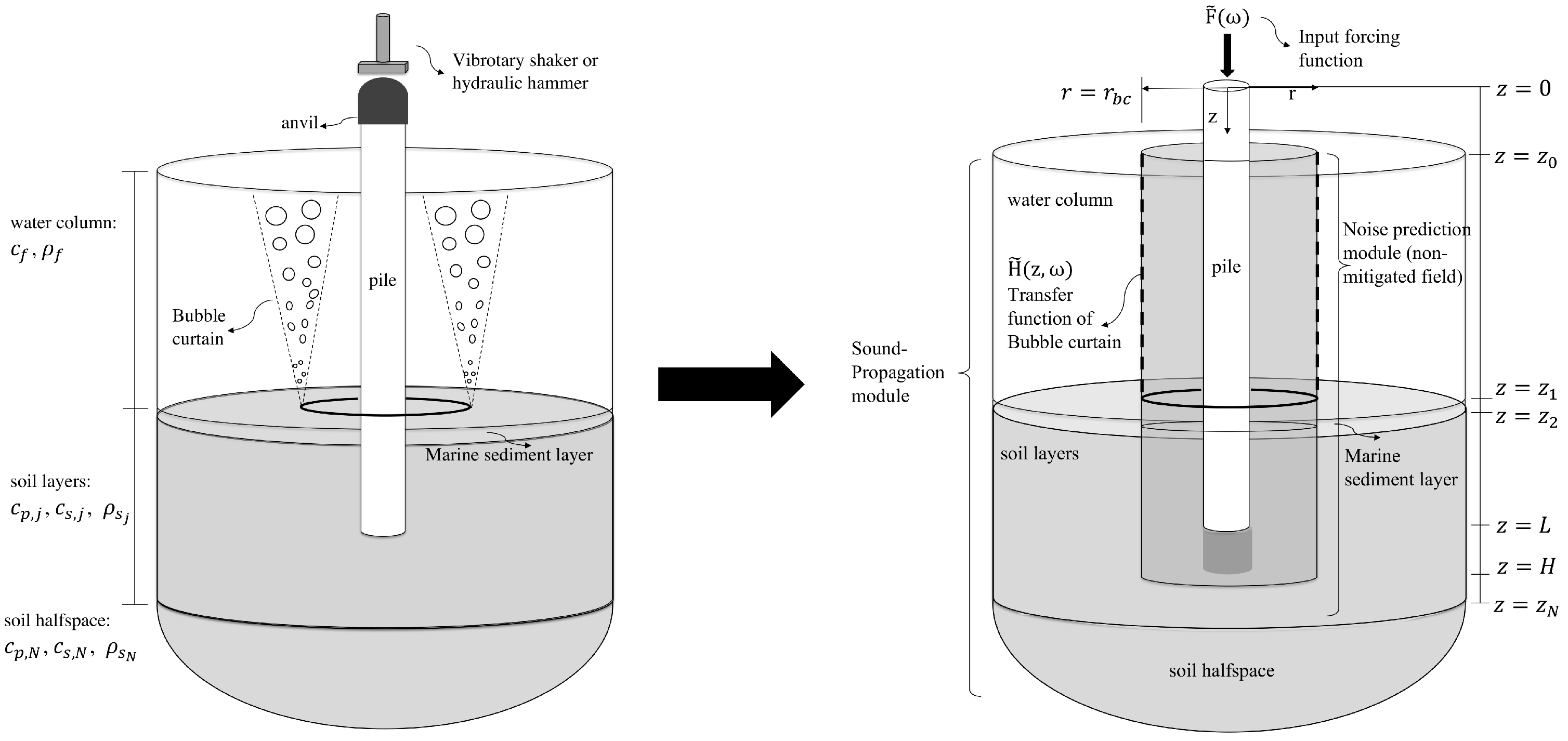
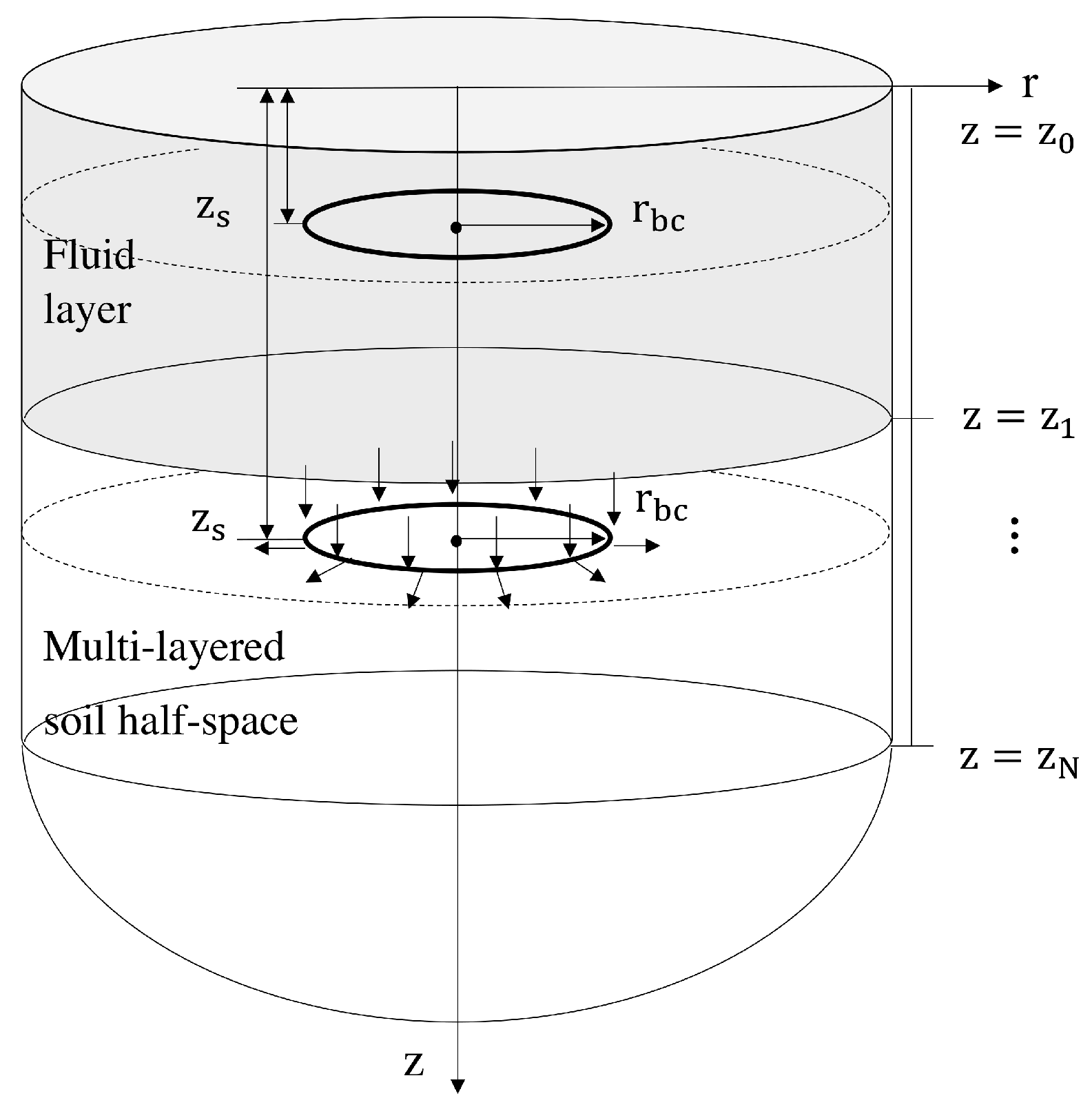
2.1. Description of the Model

As shown in Figure 1 (left), the system is composed of the foundation pile, the vibratory shaker or the hydraulic hammer, the air bubble curtain, and the surrounding seawater and sediment. It is assumed that the geometry of the domain and the boundary and interface conditions are cylindrically symmetric. The complete model consists of two modules as shown in Figure 1 (right): the noise prediction module aiming at describing the vibro-acoustic behavior of the pile–soil–water system without the presence of the air bubble curtain [29], and the noise reduction module used to describe the air bubble curtain. The noise reduction module is integrated to the noise prediction module through depth- and frequency-dependent transfer functions.
The pile is modeled as elastic thin shell described by a linear high-order shell theory [30]. The shell is then coupled to a fluid layer overlying a layered elastic waveguide through the mode matching technique [17,31]. At the top of the pile z = 0 , the load induced by the hammer is described by a vertical force. The length of the pile is L and the material constants E, ν , R, ρ , and t are the complex modulus of elasticity in the frequency domain, the Poisson ratio, the radius of the mid-surface of the shell, the density, and the thickness of the shell, respectively. The fluid is described as an ideal, linearly elastic fluid with c f being the sound speed and ρ f being the density of the water. The soil is modeled as a linear elastic continuum with c p , j , c s , j being the compressional and shear wave speeds, ρ s , j being the density of the soil with the index j = 1 , 2 , , N specifying the soil layers and the bottom soil half-space. The frequency-dependent attenuation coefficients α 1 j and α 2 j are defined as ( 20 π log 10 e ) α p j and ( 20 π log 10 e ) α s j , respectively, with α p j and α s j being the compressional and shear damping constants per layer in units of dB per wavelength. The sea surface is positioned at z = z 0 , the seabed at z = z 1 , and the various interfaces between soil layers at z = z k with k = 2 , , N . At the location of the air bubble curtain, the transmission coefficients of air bubble curtain are derived and introduced to the noise prediction model through a boundary integral formulation at r = r b c .

2.2. Governing Equations

The set of partial differential equations describing the linear vibration of the complete pile–water–soil system and the complex turbulent two-phase flow are given in time domain as
L u + I u ¨ = ( H ( z z 1 ) H ( z L ) ) t s + ( H ( z z 0 ) H ( z z 1 ) ) p f + f e · δ ( z ) , 0 < z < L
2 p f ( r , z , t ) 1 c f 2 p ¨ f ( r , z , t ) = 0 , z 0 < z < z 1 , R < r < r b c b ( z ) , r > r b c + b ( z )
( λ s j + 2 μ s j ) ( · u s j ) μ s j × ( × u s j ) = ρ s j u ¨ s j , z j < z 1 < z j + 1 , R < r <
· ( ϵ f ρ f u ¯ f × u ¯ f + ϵ f ρ f δ u f × δ u f ¯ ) = ϵ g ρ g g , z 0 < z < z 1 , r b c b ( z ) < r < r b c + b ( z )
· ( ϵ f ρ f u ¯ f ) = 0 , z 0 < z < z 1 , r b c b ( z ) < r < r b c + b ( z )
n ( v p ) t + · ( n ( v p ) u g ) = v p r 1 ( v p , v q ) n ( v q ) d v q 0 v p v q r 1 ( v p , v q ) d v q n ( v q ) v p + 1 2 v p r 2 ( v p , v p v q ) n ( v ) n ( v p v q ) d v q v p r 2 ( v p , v p v q ) n ( v q ) n ( v p ) d v q , z 0 < z < z 1 , r b c b ( z ) < r < r b c + b ( z )
In Equation (1), L and I are the stiffness and modified inertia matrices of the shell, u is the displacement vector of the mid-surface of the shell, H ( z z i ) are the Heaviside step functions, p f represents the fluid pressure exerted at the outer surface of the shell within the water column, and f e · δ ( z ) is the forcing vector representing the load applied at the top of the pile with δ ( z ) being the Dirac delta function. In Equation (2), p f ( r , z , t ) represents the pressure of the fluid with r b c being the radius of the air bubble curtain and b ( z ) being the half-width of the air bubble curtain which is a function of water depth. In Equation (3), u s j is the displacement vector of the soil layer j. In Equations (4) and (5), ϵ f and ϵ g are fluid and gas fractions, respectively; g is the gravitational constant; and u ¯ f is the mean liquid flow velocity with δ u f being its fluctuation. In Equation (6), n ( v p ) is the bubble number density with v p and v q being the bubble volumes, and r 1 ( v p , v q ) and r 2 ( v p , v q ) are the breakup and coalescence kernel functions, respectively.
At the pile–water interface, the pressure/stress equilibrium and displacement continuity are satisfied at both pile–water and pile–soil interface; the latter under the assumption of a perfect contact condition of no pile slip:
u r ( z , t ) = u f ( R , z , t ) , z 0 z z 1 u r ( z , t ) = u s ( R , z , t ) and u z ( z , t ) = w s ( R , z , t ) , z 1 z L
In Equation (7), u r and u z are the radial and vertical displacements of the shell, respectively; u f is the radial displacement of the fluid; and u s and w s are the radial and vertical displacements of the soil, respectively.
At the sea surface z = z 0 , the pressure release boundary condition is applied. At the fluid–soil interface z = z 1 , the continuity of both the vertical displacement and normal to the interface traction are applied. A rigid boundary condition is applied in the sound generation module at a great depth z = z N . In the sound propagation module, the seabed is described as a horizontally stratified elastic half-space. At the soil–soil interfaces, both stress equilibrium and displacement continuity are applied. This set of boundary and interface conditions read
p f ( r , z 0 , t ) = 0 , r R
σ z z 1 ( r , z 1 , t ) + p f ( r , z 1 , t ) = 0 , u z , f ( r , z 1 , t ) = w s 1 ( r , z 1 , t ) , σ z r 1 ( r , z 1 , t ) = 0 , r R
w s j ( r , z j , t ) = w s j 1 ( r , z j , t ) , u s j ( r , z j , t ) = u s j 1 ( r , z j , t ) , 2 j N , r R
σ z z j ( r , z j , t ) = σ z z j 1 ( r , z j , t ) , σ z r j ( r , z j , t ) = σ z r j 1 ( r , z j , t ) , 2 j N , r R
In Equations (8)–(11), u z , f are the vertical displacement components of the fluid, w s j and u s j are the vertical displacement components in the j th soil layer, and σ z z j and σ z r j being the normal and tangential stress components in the j th soil layer. Equations (1)–(11) including the radiation conditions of r describe fully the vibroacoustic of the total system in the time domain.

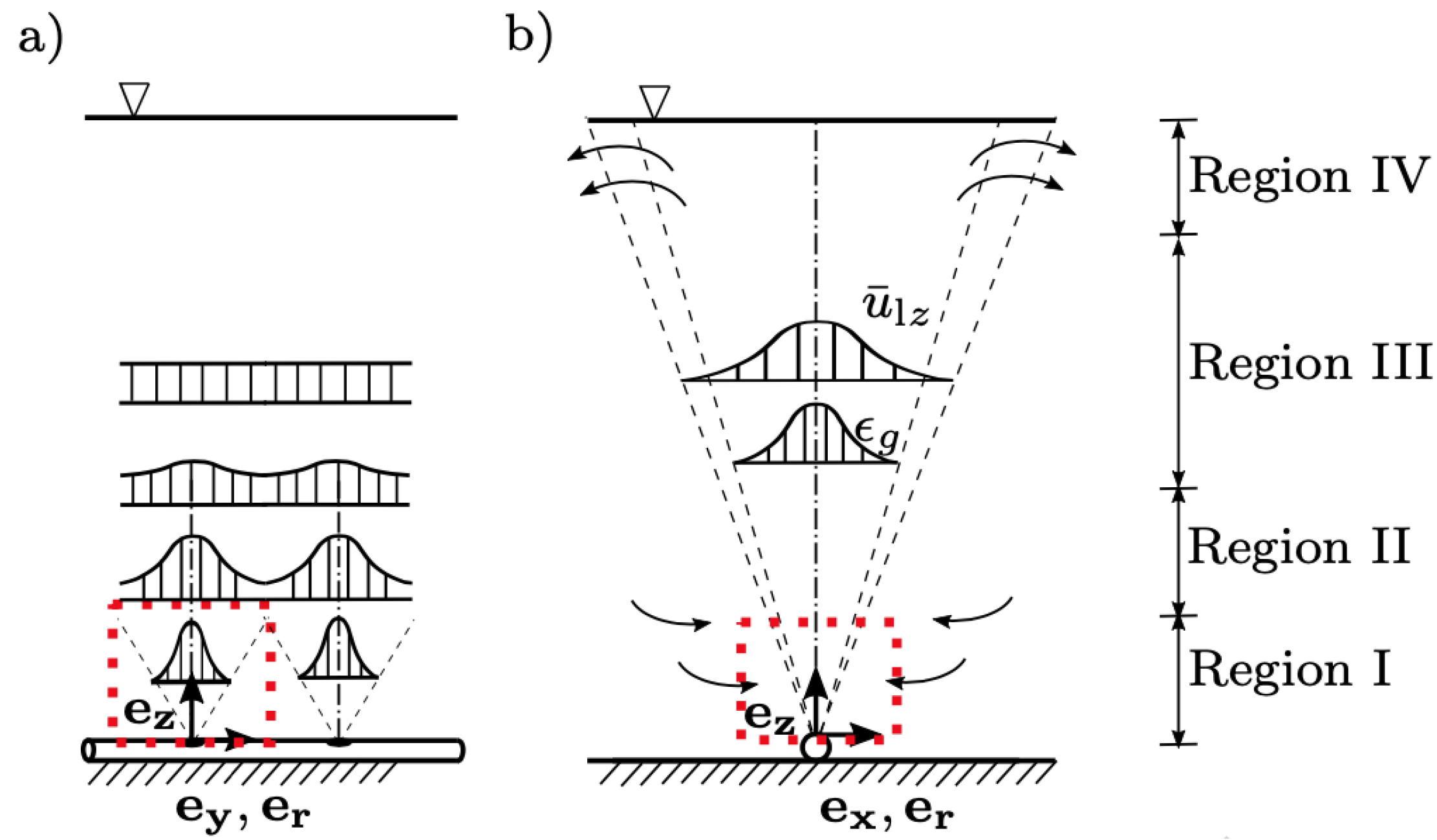
3. Noise Predictions of Non-Mitigated Field

The noise prediction model for the non-mitigated field consists of two modules. The noise source for offshore pile driving is first characterized by the sound generation module, which is based on a three-dimensional vibroacoustic noise prediction model developed earlier by Tsouvalas and Metrikine [17]. The prediction from the sound generation module has been verified against the data available in the literature from various measurement campaigns and one theoretical benchmark [21]. This module describes the dynamic response of the coupled pile–water–soil system. The eigenvalue problems of the shell and acousto-elastic waveguide are solved first. Next, the mode matching technique is applied to couple the pile to the surrounding fluid–sediment layers. A set of response functions at the location of the bubble curtain r = r b c are generated in the frequency domain, which involves pressure, velocity, displacement, and stress tensors. As the system is linear and divided into subsystems, it requires only part of the simulation to be recomputed for examining various scenarios including varying forcing functions, pile configurations, and soil conditions. Compared to FE models, the model presented herein can be used in probabilistic analysis of noise predictions involving a large number of simulations with less computational effort.
The sound propagation module is based on Green’s functions for ring sources located on the cylindrical surface at r = r b c as depicted in Figure 2. By applying the contour integration technique, the expressions of displacement potential functions Φ ˜ Ξ , ξ g ( r , z ; r b c , z s ; ω ) in frequency domain are given as a summation over a finite number of poles supplemented by the Ewing–Jardetsky–Press (EJP) branch line integrations [32], i.e.,
Φ ˜ Ξ , ξ g ( r , z ; r b c , z s ; ω ) = π i m = 1 M [ Res ( Φ ^ Ξ , ξ g ( k r ( m ) , z ; r b c , z s ) ) H 0 ( 2 ) ( k r ( m ) r ) k r ( m ) ] + 1 2 α + β Φ ^ Ξ , ξ g ( k r , z ; r b c , z s ) H 0 ( 2 ) ( k r r ) k r d k r
in which Res ( f ( k r ( m ) ) ) indicates the residue of the functions f ( k r ) at the pole k r ( m ) , H 0 ( 2 ) is the zero order Hankel function of the second kind, M indicates the number of poles with m being the index, α and β represent the branch cuts related to the branch point k p N and k s N with k p N and k s N being the compressional and shear wavenumbers, respectively.
The fundamental solutions of Green’s displacement tensors U ˜ α β Ξ ξ ( r , r s , ω ) are derived from the potential functions [33] given the receiver point at r = ( r , z ) (in medium Ξ ) in α -direction due to a unit impulse at source r s = ( r b c , z s ) (in medium ξ ) in β -direction:
U ˜ α β s ξ ( r , r s , ω ) = ϕ ˜ s j , ξ g ( r , r s , ω ) + × W , W = ψ s j , ξ g ( r , r s , ω ) r ,
U ˜ α β f ξ ( r , r s , ω ) = ϕ ˜ f , ξ g ( r , r s , ω ) .
The direct boundary element method (BEM) is adopted in this model to couple the noise prediction model for non-mitigated field and noise reduction model for the air bubble curtain as discussed in Section 4. The solution of the acousto-elastic wavefield employs Somigliana’s identity in elastodynamics and Green’s third identity in potential theory [33,34,35]. The response functions from the noise prediction model are coupled to the sound propagation module through a boundary integral formulation on the cylindrical boundary surface r = r b c . By utilizing Betti’s reciprocal theorem in elastodynamics [34] and Green’s theorem for acoustic problem [35], the complete solution for the acousto-elastic domain reads
u ˜ α Ξ ( r , ω ) = u ˜ α Ξ , f ( r , ω ) + u ˜ α Ξ , s ( r , ω ) = β = r , z S s H ˜ ( z , ω ) ( U ˜ α β Ξ s ( r , r b c , ω ) · t ˜ β n ( r b c , ω ) T ˜ α β n , Ξ s ( r , r b c , ω ) · u ˜ β ( r b c , ω ) ) d S s ( r b c ) + S f ( U ˜ α r Ξ f ( r , r b c , ω ) · p ˜ ( r s , ω ) T ˜ α r n , Ξ f ( r , r s , ω ) · u ˜ r ( r b c , ω ) ) d S f ( r b c ) , r V
in which n is the outward normal to the cylindrical boundary, H ˜ ( z , ω ) is the transmission coefficient function of the air bubble curtain with depth and frequency dependence as discussed in Section 4.

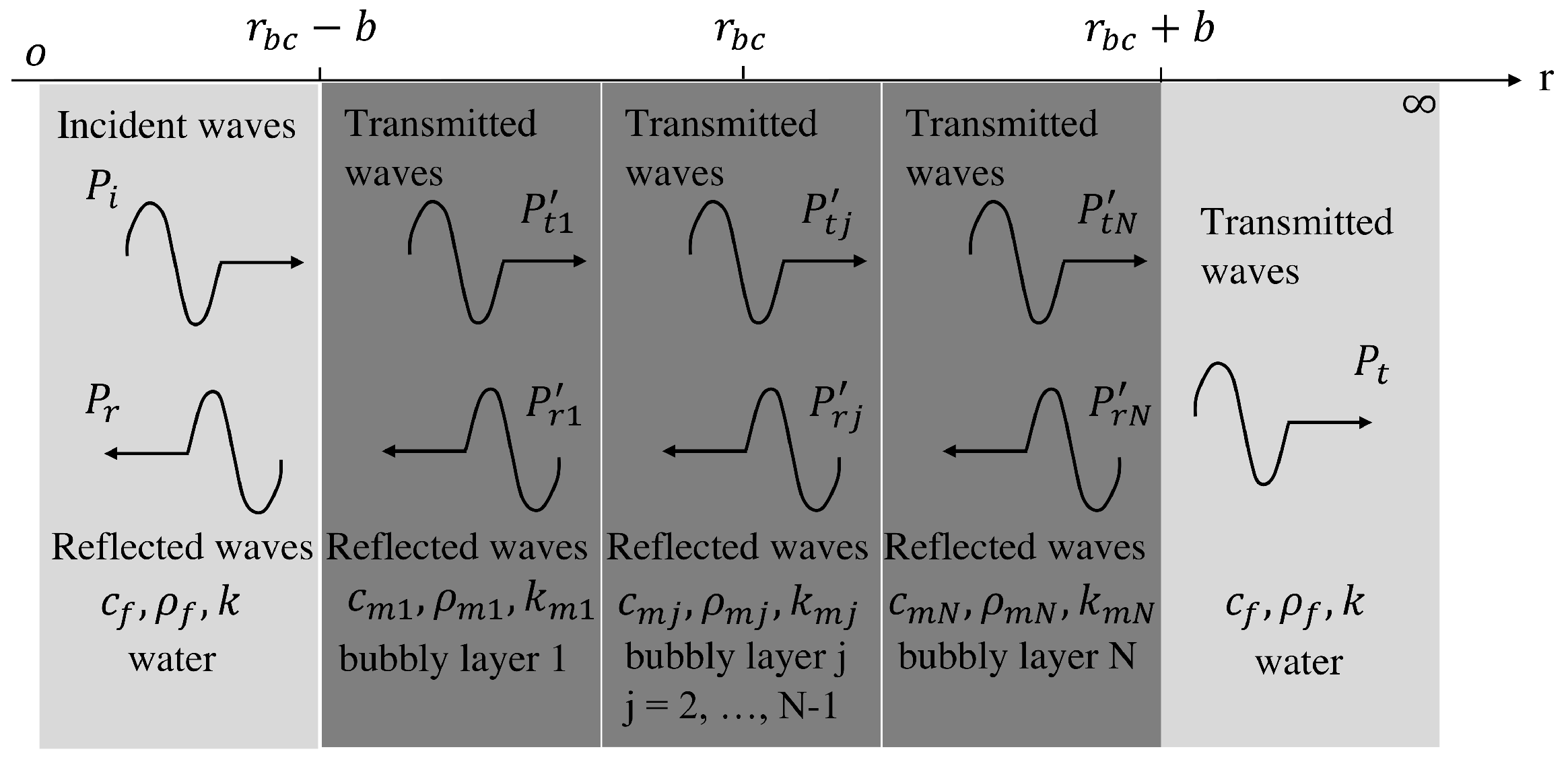
4. Modeling the Air Bubble Curtain

In this section, a one-way coupling noise reduction module for capturing acoustic properties of the air bubble curtain is derived. The local wavenumber distribution is based on a fluid dynamic model developed by Bohne et al. [27], in which a turbulent two-phase bubble flow is well captured especially in the vicinity of the nozzle where a high gas fraction is present. Based on the distribution of the local effective wavenumbers over the entire water depth, the depth- and frequency-dependent transmission coefficients are obtained by a simplified one-dimensional acoustic wave propagation approach developed by Commander and Prosperetti [36]. The noise reduction module is coupled to the free-field noise prediction model through a boundary integral formulation as given by Equation (15).

4.1. Local Effective Wavenumber in a Bubble Curtain

To obtain the local effective wavenumber of the air bubble curtain, the model developed by Bohne et al. [27] is used. The governing equations based on momentum balance of the gas–liquid mixture, the conservation of mass of the liquid phase and population balance of a turbulent flow are already introduced in Equations (4)–(6). The bimodal bubble size distribution is introduced by Lethr et al. [37] with observations of small and large bubbles especially in the vicinity of the nozzle as depicted in Figure 3. The detailed derivation is given in [27,38] and is omitted here for the sake of brevity. The initial conditions for the bubble formation process are given as
u l z m 0 = 2 M 0 ( 2 λ 2 + 1 ) γ b 0 2 ρ f π ( 2 ϵ g m 10 λ 2 + 2 ϵ g m 20 λ 2 2 λ 2 1 )
b 0 = m ˙ 0 ( λ 2 + 1 ) λ 2 π ρ g 0 ( λ 2 + 1 ) ( ϵ g m 10 u r e l 1 ( v ¯ 10 ) + ϵ g m 20 u r e l 2 ( v ¯ 20 ) ) + λ 2 u l z m 0 π ρ g 0 ( ϵ g m 10 + ϵ g m 20 )
ϵ g m 10 = 0.005
ϵ g m 20 = 0.495
v ¯ 20 = 4 3 π ( 1.1447 a prim ) 3
v ¯ 10 = v ¯ 20 30
with the initial centerline velocity u l z m 0 , the half width of the bubble curtain b 0 , the initial gas fraction of the small bubble ϵ g m 10 , the initial gas fraction of the large bubble ϵ g m 20 , the initial arithmetic mean bubble volume of the small bubbles v ¯ 10 , and the initial arithmetic mean bubble volume of the large bubbles v ¯ 20 . u r e l 1 ( v ¯ 1 ) and u r e l 2 ( v ¯ 2 ) are the relative velocities between the upward rising air bubbles and the mean flow of the fluid, which are functions of the local mean bubble size of each gas phase [39,40]. M 0 is the initial momentum of the mixture and d prim is the diameter of the primary bubble, which are quantified at the nozzle as [38,41]
M 0 = q n ρ g n u g n + 2 q n u g n ( ρ f ρ g n ) g · ( 6.2 d n )
d prim = 1 2 [ 1.3 ρ f ( q n / d prim ) 2 + π d n σ + 15 η q n / d prim ( ρ f ρ g n ) 6 π ] 1 / 3
in which u g n is the gas velocity in the nozzle, q n is gas volume rate in the nozzle, and ρ g n is the density of gas in the nozzle. In Equation (), d prim is solved for by an iterative method. Derived from the Equations (4)–(6) and assuming Gaussian distributions of the mean fluid velocity and gas fractions, the resulting set of equations read
d d z ( m ( u , z ) ) = q ( u , z )
In Equation (24), u = [ u l z m , b , ϵ g m 1 , ϵ g m 2 , v ¯ 1 , v ¯ 2 ] T represents the vector of six unknowns, in which u l z m is the centerline velocity, b is the half width of the bubble curtain, ϵ g m 1 is the gas fraction of the small bubble, ϵ g m 2 is the gas fraction of the large bubble, v ¯ 1 is the arithmetic mean bubble volume of the small bubbles, and v ¯ 2 is the arithmetic mean bubble volume of the large bubbles. To solve the set of first order partial differential equations, the forward Euler method is used for integration along the z-coordinate with the initial condition given in Equations (16)–(20). Once the set of Equations (24) is solved, u are obtained as depth-dependent fluid dynamic properties, which will be used in Equation (44) to determine the local effective wavenumber and subsequently in Equation (56) to determine the transmission coefficient functions of the air bubble curtain.
The elements of the integral fluxes m ( u , z ) = [ m 1 , m 2 , m 3 , m 4 , m 5 , m 6 ] T read
m 1 ( u , z ) = 2 π γ ρ f u l z m 2 ( b 2 4 ϵ g m 1 λ 2 b 2 2 ( 2 λ 2 + 1 ) ϵ g m 2 λ 2 b 2 2 ( 2 λ 2 + 1 ) )
m 2 ( u , z ) = 2 π ρ f u l z m ( b 2 4 ϵ g m 1 λ 2 b 2 2 ( 2 λ 2 + 1 ) ϵ g m 2 λ 2 b 2 2 ( 2 λ 2 + 1 ) )
m 3 ( u , z ) = 2 π ρ g ( z ) ϵ g m 1 ( u l z m λ 2 b 2 2 ( 2 λ 2 + 1 ) + g Δ ρ 3 μ ( v ¯ 1 0.21 ) ( 2 3 ) λ 2 b 2 2 )
m 4 ( u , z ) = 2 π ρ g ( z ) ϵ g m 2 ( u l z m λ 2 b 2 2 ( 2 λ 2 + 1 ) + g Δ ρ 3 μ ( v ¯ 1 0.68 ) ( 2 3 ) λ 2 b 2 2 )
m 5 ( u , z ) = 2 π ρ g ( z ) ϵ g m 1 v ¯ 1 ( u l z m λ 2 b 2 2 ( 2 λ 2 + 1 ) + g Δ ρ 3 μ ( v ¯ 1 0.21 ) ( 2 3 ) λ 2 b 2 2 )
m 6 ( u , z ) = 2 π ρ g ( z ) ϵ g m 2 v ¯ 2 ( u l z m λ 2 b 2 2 ( 2 λ 2 + 1 ) + g Δ ρ 3 μ ( v ¯ 1 0.68 ) ( 2 3 ) λ 2 b 2 2 )
with Δ ρ being the difference between the density of fluid and air, μ = 10 3 N · s / m 2 being the viscosity of the fluid, and γ = 1 being the amplification factor.
Similarly, the elements of the integral source terms q ( u , z ) = [ q 1 , q 2 , q 3 , q 4 , q 5 , q 6 ] T are
q 1 ( u , z ) = π g ρ f λ 2 b 2 ( ϵ g m 1 + ϵ g m 2 )
q 2 ( u , z ) = 2 π α ρ f u l z m b
q 3 ( u , z ) = Z 2 ρ g ( z ) π λ 2 b 2 ϵ g m 2 0.9024 r 2 ( ϵ g m 1 , ϵ g m 2 , v ¯ 2 , 5 v ¯ 1 ) ρ g ( z ) ϵ g m 1 ϵ g m 2 π λ 2 b 2 v ¯ 2 3.1043 π 2 r 2 ( ϵ g m 1 , ϵ g m 2 , v ¯ 1 , v ¯ 1 ) ρ g ( z ) ϵ g m 1 2 λ 2 b 2
q 4 ( u , z ) = Z 2 ρ g ( z ) π λ 2 b 2 ϵ g m 2 + 0.9024 r 2 ( ϵ g m 1 , ϵ g m 2 , v ¯ 2 , 5 v ¯ 1 ) ρ g ( z ) ϵ g m 1 ϵ g m 2 π λ 2 b 2 v ¯ 2 + 3.1043 π 2 r 2 ( ϵ g m 1 , ϵ g m 2 , v ¯ 1 , v ¯ 1 ) ρ g ( z ) ϵ g m 1 2 λ 2 b 2
q 5 ( u , z ) = Z 1 v ¯ 1 ρ g ( z ) π λ 2 b 2 ϵ g m 1 0.9024 r 2 ( ϵ g m 1 , ϵ g m 2 , v ¯ 2 , 5 v ¯ 1 ) ρ g ( z ) ϵ g m 1 ϵ g m 2 π λ 2 b 2 v ¯ 2 v ¯ 1 + 0.3463 π 2 r 2 ( ϵ g m 1 , ϵ g m 2 , v ¯ 1 , v ¯ 1 ) ϵ g m 1 2 λ 2 b 2 + 3.1043 π 2 r 2 ( ϵ g m 1 , ϵ g m 2 , v ¯ 1 , v ¯ 1 ) ρ g ( z ) ϵ g m 1 2 λ 2 b 2 v ¯ 1
q 6 ( u , z ) = 2 Z 2 v ¯ 2 ρ g ( z ) π λ 2 b 2 ϵ g m 2 + 1.8048 r 2 ( ϵ g m 1 , ϵ g m 2 , v ¯ 2 , 5 v ¯ 1 ) ρ g ( z ) ϵ g m 1 ϵ g m 2 π λ 2 b 2 + 0.4250 π 2 r 2 ( ϵ g m 1 , ϵ g m 2 , v ¯ 2 , v ¯ 2 ) ρ g ( z ) ϵ g m 2 2 λ 2 b 2 + 3.1043 π 2 r 2 ( ϵ g m 1 , ϵ g m 2 , v ¯ 1 , v ¯ 1 ) ρ g ( z ) ϵ g m 1 2 λ 2 b 2
with r 2 is the function of the air fraction and arithmetic mean bubble volume of the small and large bubbles as given in [27]. The density of the gas is a function of height from the nozzle based on an ideal gas law.
As the vertical distances from the nozzle increase, both the gas fraction ratio and the arithmetic mean bubble volume of large bubbles drop significantly and approach zero, and part of the components in the vector q are modified as
q 3 ( u , z ) = q 4 ( u , z ) = 0
q 5 ( u , z ) = Z 1 v ¯ 1 ρ g ( z ) π λ 2 b 2 ϵ g m 1 + 0.3463 π 2 r 2 ( ϵ g m 1 , ϵ g m 2 , v ¯ 1 , v ¯ 1 ) ϵ g m 1 2 λ 2 b 2
q 6 ( u , z ) = Z 2 v ¯ 2 ρ g ( z ) π λ 2 b 2 ϵ g m 2 + 0.9024 r 2 ( ϵ g m 1 , ϵ g m 2 , v ¯ 2 , 5 v ¯ 1 ) ρ g ( z ) ϵ g m 1 ϵ g m 2 π λ 2 b 2 + 0.4250 π 2 r 2 ( ϵ g m 1 , ϵ g m 2 , v ¯ 2 , v ¯ 2 ) ρ g ( z ) ϵ g m 2 2 λ 2 b 2
while the other components remain the same.
Once the depth-dependent vector u is known, the local bubble number density distribution are obtained by subdividing them into a fraction of large bubbles and a fraction of small bubbles
n ( u , r , z , a ) = n 1 ( u , r , z , a ) + n 2 ( u , r , z , a )
with the equilibrium bubble radius a and the bubble number density n ( u , r , z , a ) . The bubble number density distribution for the small bubble fraction n 1 ( u , r , z , a ) is approximated by a lognormal distribution and the large bubble fraction n 2 ( u , r , z , a ) by an exponential distribution [37],
n 1 ( u , r , z , a ) = ϵ g 1 ( r , z ) v ¯ 1 2 2 π v ¯ 1 3 v ( a ) exp ( 2 9 l n ( e 9 / 8 v ( a ) v ¯ 1 ) )
n 2 ( u , r , z , a ) = ϵ g 2 ( r , z ) v ¯ 2 2 exp ( v ( a ) v ¯ 2 )
The gas fraction for both small and large bubbles is range- and depth-dependent as
ϵ g i ( r , z ) = ϵ g m i ( z ) exp ( r 2 λ 2 b 2 )
The local effective wavenumber is written as
k m 2 ( ω , r , z ) = ω 2 c f 2 + 4 π ω 2 0 a n ( u , r , z , a ) ω 0 2 ( z , a ) ω 2 + 2 i β ( z , a ) ω d a
with the angular frequency ω . The natural angular frequency ω 0 ( z , a ) and the damping constant β ( z , a ) are defined as [36]
ω 0 ( z , a ) = p g ( z ) ρ f a 2 ( 3 2 σ p g ( z ) a )
β ( z , a ) = γ 0 1 10 γ 0 · p g ( z ) ρ f D + 2 μ ρ f a 2
in which σ = 0.073 N/m is the surface tension of the water, γ 0 = 1.41 is the ratio of specific heats, and D = 1.9 × 10 5   m 2 / s is the gas thermal diffusivity.

4.2. Local Transmission Coefficients of a Bubble Curtain

To obtain the sound transmission characteristics of a bubble curtain, a model for determining the depth- and frequency-dependent transmission coefficient of an air bubble curtain is developed, which is based on the approach of Commander and Prosperetti [36]. Consider an incident sinusoidal wave as shown in Figure 4, the field is solely r-dependent and the bubbly mixture occupies the region r b c b < r < r b c + b with r b c being the location of the air bubble curtain and b being the half width varying with height from the nozzle as discussed in Section 4.1. The water column and air bubble curtain are divided into M regions along the vertical coordinate. At each vertical domain, a one-dimensional problem is considered with an input incident wave and properties of the layers. The transmission coefficients are determined per z-coordinate and is constant within the vertical step size of the integration. The bubble layer is divided into N b c layers as depicted by the gray area in Figure 4. These assumptions allow for the simplification of the solutions for the transfer coefficients of the bubbly layer. The focus is placed on the energy transmission through air bubble curtain, the back-scattering effect is not considered in this model. The solutions of the pressure fields in three regions are expressed as [35]
P L ( r , ω ) = P i + P r = A 1 exp ( i k r ) + A 2 exp ( i k r ) , r < r b c b
P B C , j ( r , ω ) = P t j + P r j = B 1 j exp ( i k m j r ) + B 2 j exp ( i k m j r ) , r b c b < r < r b c + b
P R ( r , ω ) = P t = C 1 exp ( i k r ) , r > r b c + b
In Equations (47)–(49), the local effective wavenumber k m j is obtained by Equation (44) at layer j, P L , P B C , j , and P R are the left-, air bubble curtain, and the right-pressure field, respectively. P i is the incident plane wave propagating in the positive r-direction in the fluid, P r is the reflected wave traveling in the negative r-direction in the fluid, similarly, P t j and P r j are the forward- and backward-propagating waves in the bubbly mixture of layer j, P t is the transmitted wave in the fluid on the right side of the bubbly mixture. The solutions assume a time dependence exp(i ω t).
At the interface between the bubbly mixture and seawater, and between bubbly layers, the continuity of the pressure and normal velocity is required as [36]
p f = p m 1 , p f = p m N b c , p m j = p m ( j + 1 ) , j = 1 , , N b c 1
v r , f = v r , m 1 , v r , f = v r , m N b c , v r , m j = v r , m ( j + 1 ) , j = 1 , , N b c 1
In Equation (50), p f and v r , f are the pressure and the radial velocity in the fluid, respectively, and p m and v r , m are the pressure and the radial velocity in the bubbly mixture. The radial velocity is defined as
v r , i = 1 i ω ρ i p i r
with the subscript i being f or m represents the fluid layer or bubbly layer. In the work of Commander and Prosperetti [36], the density of the bubbly mixture was approximated by the density of water. However, in Equation (52), the density of the bubbly mixture is characterized by the depth-dependent gas and fluid fraction coefficients as derived from solving Equation (24) as discussed in Section 4.1.
The set of 2N+2 interface conditions reads
P L ( r b c b , ω ) = P B C , 1 ( r b c b , ω ) , v r , f ( r b c b , ω ) = v r , m 1 ( r b c b , ω )
P B C , j ( r b c , j , ω ) = P B C , j + 1 ( r b c , j , ω ) , v r , m j ( r b c , j , ω ) = v r , m ( j + 1 ) ( r b c , j , ω )
P B C , N b c ( r b c + b , ω ) = P R ( r b c + b , ω ) , v r , f ( r b c + b , ω ) = v r , m N b c ( r b c + b , ω )
in which r b c , j = r b c b + 2 b ( j 1 / 2 ) / N b c , j = 1 , , N . By substituting the expressions in Equations (47)–(49) into the interface conditions at r = r b c ± b and r = r b c , j , and assuming an incident wave of unit amplitude A 1 = 1 , the amplitude coefficients A 2 , B 1 j , B 2 j , and C 1 are obtained.
Next, the solutions are generalized for depth-dependent acoustic properties of the air bubble curtain including the half-width b ( z ) and effective medium wavenumber k m ( ω , z ) . The local transfer coefficient of the bubbly layer is defined by
H ˜ ( z , ω ) = C 1
The transfer coefficient function in Equation (56) is coupled to the noise prediction model through boundary integral equation in Equation (15). The local transmission loss (dB/m) is obtained as
T L ( z , ω ) = 10 log | C 1 | 2

5. Validation Study of the Effective Wavenumber Model

For the validation of the integral model for the effective wavenumber, the modeling results are compared to the numerical solutions by Bohne et al. [27] and measurement data from the experiment by Milgram [38]. The input parameters of the air bubble curtain system are given in the Table 1.
The experiment took place at a lake with a water depth T of 50 m at a local sinkhole spring in Florida, which fits the typical bathymetry of offshore pile-driving environment (shallow water up to 40–50 m water depth) with the application of an air bubble curtain system. Three air flow rates involving 0.024, 0.283, and 0.59 m 3 /s at atmospheric are examined. In Figure 5, the comparison of centerline velocities and half width of the bubbly layer are shown for the numerical results from literature and measured data set from the experiments [27,38]. The numerical evaluation of both centerline velocity and half width of the bubble curtain shows a relatively good agreement with the experiment, the small deviation from Bohne’s model can be due to different numerical integration scheme and entrainment coefficient to achieve better fitting to the measured data set. As can be seen in Figure 5 (left), the velocities decrease slowly as the distance from the nozzle increases. The maximum velocities are observed in the vicinity of the nozzle. In Figure 5 (right), the width of the bubble plume is found to increase linearly with height above the nozzle, which is also in line with the observation of cone shaped bubbly mixture in offshore pile installation campaign with the application of the bubble curtain system.
In Figure 6, the mean bubble volume and gas fraction ratio of both small and large bubbles are presented. Different fluid dynamic behaviors are observed for the large and small bubbles with the varying height from the nozzle. As the height from the nozzle increases, large bubbles break up into smaller ones as the gas fraction ratio of the small bubble increases while the volume of the large bubbles approaches the one of the small bubbles. The module captures the bubble formation process especially in the vicinity of the nozzle and forms the basis for calculation of more accurate acoustic properties of the air bubble curtain.
To validate the derivation of the transmission coefficients of the air bubble curtain, the modeled results are compared to the measured transmission loss obtained in the freshwater lake experiment [42]. The water depth T is 9.7 m. The case with air flow rate being 0.0019 m 2 /s, nozzle interval Δ y n = 25 cm, and nozzle size being d n = 1.4 mm is evaluated. For the comparison of the different models and experiment data set, the overall transmission loss is defined as
T L b c ( ω ) = 10 log [ 1 N z | C 1 | 2 Δ z T ]
In Equation (58), the rule of thumb for using six elements per wavelength is applied for the vertical step size Δ z .
As shown in Figure 7, the air bubble curtain model improves its performance as for the higher frequencies the transmission loss is close to the measured data, and it does not require any assumption of the bubble size distribution coefficients [27]. As indicated by the black solid line, the model is more in line with the measurement data compared to other numerical model for frequencies below 500 Hz, which is mainly due to the choice of the initial condition and control parameters including the spreading coefficients and the entrainment factor. Frequencies below 500 Hz are also important in offshore pile driving.

6. Validation Study of the Complete Model Including the Air Bubble Curtain

In this section, the model predictions are validated against measurement data collected from an offshore wind farm constructed in 2018 (hereafter referred to as project A). In Table 2, the material and geometrical parameters are estimated from the available geotechnical reports at the pile installation site.

6.1. Maximum Noise Reduction Level

To predict the maximum noise reduction levels that can be achieved by the air bubble curtain at the pile installation site, three scenarios are considered to distinguish the water- and soilborne noise transmission paths:
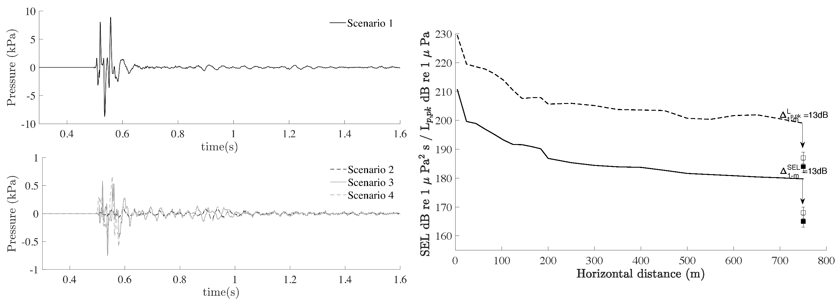
  • scenario 1—noise prediction without the presence of air bubble curtain (base case);
  • scenario 2—elimination of the waterborne path at the position of the air bubble curtain leaving the propagation of the waves through the soil unaffected; and
  • scenario 3—same as scenario 2 but with an additional 1 m gap at the lowest part of the seawater column in which the noise presumably leaks.
In scenario 2, the noise sources in the water column are effectively canceled (100% cancellation of the waterborne path) while the field in the soil is propagated undisturbed in the exterior (to the air bubble curtain) domain. This allows one to estimate the maximum noise reduction potential that a noise mitigation system can achieve with a theoretical efficiency of 100% in blocking the waterborne path. The difference between the results of the non-mitigated noise field (scenario 1) and the ones at which the waterborne path is fully or partially blocked (scenarios 2 and 3) give an estimate of the maximum noise reduction that can be achieved by eliminating the entire noise transmission path in the fluid and provide a clear indication of the influence of the zone of flow establishment in the vicinity of the nozzles (Region I depicted in the Figure 3). Considering the possibility to eliminate the waterborne noise sources at any distance of interest, i.e., 10 m, 50 m, etc., the distance has been chosen here equal to the one of which the outer air bubble curtain was placed ( 145 m from the pile surface).
The Peak Level ( L p , p k ) in the unit of dB re 1 µPa is determined by the absolute maximum of the sound pressure following a single hammer blow:
L p , p k = 20 log ( p p k p 0 )
In Equation (59), p p k is the zero-to-peak sound pressure and p 0 = 10 6 Pa is the reference underwater sound pressure level. The sound exposure level SEL in units of dB re 1 µ P a 2   s is defined as in [43]
SEL = 10 log ( 1 T 0 T 1 T 2 p 2 ( t ) p 0 2 d t )
with T 1 and T 2 being the starting and ending of the predicted time signature with the sound event in between and T 0 = 1 s.
The peak pressure level ( L p , p k ) and sound exposure level (SEL) of receiver points at radial distances up to 750 m are obtained here for the non-mitigated field (scenario 1) as shown in Figure 8 (left). Through an indirect method, the noise reduction level achieved by the Noise Mitigation Systems can be examined by comparing the sound levels of the non-mitigated and mitigated fields. In Figure 8 (right), the evolution of the pressure field in time is shown for a point positioned 2 m above the seabed at various radial distances from the pile for scenarios 1–3. The numerical results for the three scenarios and the comparison to the measurement are summarized in Table 3. The measured SEL and L p , p k are derived from the data collected from four hydrophones located at four difference angles as shown in Figure 9.
The range of the sound levels is given in Table 3 with their arithmetic mean values indicated in the parenthesis. The deviation of the sound levels in the measured data can be due to the existence of the currents and angular-dependent bathymetry changes in the offshore environment.
The maximum noise reduction level of ~30.0 dB in terms of SEL and ~35.0 dB in terms of L p , p k can be achieved, respectively, when the air bubble curtain blocks the entire waterborne path (scenario 2). With the consideration of 1 m gap due to the bubble formation process in the vicinity of the nozzle (scenario 3), the predicted ideal noise reduction level by an air bubble curtain reduce to ~20.9 dB for SEL and ~21.4 dB for L p , p k .
The energy flux is given at the location of the outer bubble curtain r = r b c , 2 = 145 m. As can be seen in Figure 10, close to the seabed the amount of the energy is relatively high compared with the entire water depth and soil depth, which indicates that a great amount of energy could channel from the vicinity of the seabed back into the water column due to the thin air bubble layer close to the seabed. This also explains the difference in the noise reduction level of SEL and L p , p k between Δ 1 2 and Δ 1 2 .

6.2. Validation of the Noise Reduction with the Model of the Air Bubble Curtain

In this section, the validation of the complete model including the double air bubble curtains (DBBC) is performed, which is considered as scenario 4 hereafter. The model is based on the configuration of an offshore pile installation campaign in 2018. The installation was executed for the pile with using double big bubble curtains (DBBC), which are especially often used for large water depths (>30 m). Within the same offshore wind farm, another installation was executed for the pile without using any noise mitigation system, which has been used for the validation of the noise prediction model developed in [29]. The input parameters of the air bubble curtain system are given in Table 4, while the material and geometrical parameters are those summarized already in Table 2. The layout of the DBBC system is shown in Figure 9, where r b c , 1 and r b c , 2 are the radius of the bubble curtain with the width being b b c , 1 ( z ) and b b c , 2 ( z ) , respectively.
Based on the configuration of the bubble curtain system, the fluid dynamic and acoustic properties of the system are obtained first by the noise reduction module. Figure 11 shows the variation of the centerline velocity, width and total gas fraction of the bubble curtain over the depth. The transmission loss of the bubble curtain is derived as discussed in Section 4.2. As shown in Figure 12 (left), the mitigation is less effective at low frequencies (<100 Hz). The variation of the damping coefficients along the entire water depth in Figure 12 (right) shows that the attenuation is depth-dependent and reduces in the vicinity of the nozzle especially for the higher frequencies due to the zone of the flow establishment in the bubble formation process.
Next, the noise source for the impact pile driving is generated by the noise prediction model for non-mitigated field and is propagated first to the location of the inner air bubble curtain at r = r b c , 1 . The direct BEM is used to couple the noise prediction model for non-mitigated field and noise reduction model for the air bubble curtain as discussed in Section 4. The wavefield is then propagated to the location of the outer air bubble curtain at r = r b c , 2 and is coupled to the noise reduction model for the outer air bubble curtain through the BEM. The direct BEM gives us great flexibility to couple the non-mitigated field to a single or double air bubble curtains.
The calculated SEL and L p , p k are summarized in Table 5 compared to the measurement data collected during the pile installation campaign. The sound reduction predicted including the modeling of double air bubble curtains are ~20 dB for SEL and ∼21 dB for L p , p k at a distances of 750 m.
The summary of the noise prognosis for the offshore campaign is given in Table 5 in terms of the SEL and the L p e a k . The difference between the noise reductions for scenario 2 and 3 is due to the 1 m gap in the fluid, which can lead to the channeling of great energy in the vicinity of the seabed back into the water column as indicated in Figure 10. The noise reduction for SEL achieved by DBBC is slightly lower than the reduction by scenario 3, as scenario 3 leads to a more conservative estimation by assuming the full blockage of the transmission in the fluid domain except the 1 m gap close to the seabed. Because the air bubble curtain system has a much higher damping coefficient higher frequencies, the system works more efficient in reducing the impulsiveness of the incoming waves as evaluated by L p , p k . The deviation (3 ± 2 dB) in the measured SEL and L p , p k from hydrophones at different angles indicates the influence of the ocean currents and three dimensional effects of the ocean environment on the sound propagation. The ocean currents can modify the local air bubble distribution along the entire water depth, which can significantly influence the transmission coefficients of the air bubble curtain. The angle-dependent varying bathymetry may also result in various sound transmission paths at different angles of the field. The deviation of 2 dB is considered as measurement errors from the set-up of the test equipment, including the hydrophones and calibrators. The prediction of SEL by scenario 4 including the DBBC ( Δ 1 D B B C =20 dB) and the scenario 3 ( Δ 1 3 = 21 dB) are around 3 and 4 dB above the upper bound of the measured data ( Δ 1 m = 15 + 2 = 17 dB), respectively. The noise reduction L p , p k from the measurement data is much lower compared to both scenario 3 and the scenario 4 (DBBC), which indicates that both scenarios lead to conservative predictions. Further investigations regarding the sensitivity of the parameters of air bubble curtain system and the influence of currents and other environmental factors are needed to provide a better estimation of the sound pressure levels and to optimize the use of the air bubble curtain system.

7. Conclusions

This paper establishes a computationally efficient approach for noise reduction prediction in offshore pile driving with the application of a single or double air bubble curtain system. The complete model consists of two modules: the noise prediction module that describes the vibroacoustic behavior of the pile–soil–water interaction and propagates the wave field at larger distance from the pile, and the noise reduction module that describes the acoustic properties of an air bubble curtain. The solution approach is presented with the complete mathematical statement of the coupled vibroacoustic pile–water–soil system including the dynamics of the air bubble cloud. The direct boundary integral equation (BIE) formulation is used to couple the three modules and propagate the wavefield from the vicinity of the pile to the location of the inner and outer bubble curtains and to the larger distances. The validation of the local effective wavenumber model is performed by comparison to available numerical solutions and reported experimental data sets. Noise predictions are then performed for a pile installation campaign with the use of DBBC in 2018 and the results are compared to measurement data. The maximum noise reduction level of an ideal noise mitigation system is studied by eliminating the waterborne transmission path. The results indicate the maximum potential of the noise mitigation systems applied in the water column. The model can latter be used for optimization of the air bubble curtain system in order to improve the deployment strategy of the system. The modeling approach can be applied for modeling different noise mitigation techniques, which provides possibilities to examine the optimal combination of various noise mitigation techniques and position of the deployment of the system.

Author Contributions

Y.P. is the main author of this paper. Supervision, methodology, review and editing, A.T.; review and data resources, T.S.; methodology and final review, A.M. All authors have read and agreed to the published version of the manuscript.

Funding

This research was funded by China Scholarship Council (CSC) for financing the research project (201707720006) on the development of a generic underwater noise prediction model for offshore activities.

Data Availability Statement

Not applicable.

Acknowledgments

The authors wish to express their thanks to Van Oord and specifically to Remco Huizer, Wouter Dirks, and Roeland Ris for supporting this research and for providing data from a recent offshore installation campaign. For questions related to the data please contact the Noise Desk of Van Oord ([email protected]).

Conflicts of Interest

The authors declare no conflict of interest.

References

  1. Bailey, H.; Senior, B.; Simmons, D.; Rusin, J.; Picken, G.; Thompson, P.M. Assessing underwater noise levels during pile-driving at an offshore windfarm and its potential effects on marine mammals. Mar. Pollut. Bull. 2010, 60, 888–897. [Google Scholar] [CrossRef]
  2. Bundesamt fur Seeschifffahrt und Hydrographie (BSH). Standard Investigation of the Impacts of Offshore Wind Turbines on the Marine Environment (StUK4); Technical Report 7003; German Federal Maritime and Hydrographic Agency: Hamburg, Germany, 2013.
  3. Office of Protected Resources, National Marine Fisheries Service. Technical Guidance for Assessing the Effects of Anthropogenic Sound on Marine Mammal Hearing: Underwater Acoustic Thresholds for Onset of Permanent and Temporary Threshold Shifts; Technical Report; NOAA Technical Memorandum NMFS-OPR-55; U.S. Department of Commerce, National Oceanic and Atmospheric Administration: Silver Spring, MD, USA, 2016.
  4. Stöber, U.; Thomsen, F. Effect of impact pile driving noise on marine mammals: A comparison of different noise exposure criteria. J. Acoust. Soc. Am. 2019, 145, 3252. [Google Scholar] [CrossRef] [PubMed]
  5. Tsouvalas, A. Underwater Noise Emission Due to Offshore Pile Installation: A Review. Energies 2020, 13, 3037. [Google Scholar] [CrossRef]
  6. Reinhall, P.G.; Dahl, P.H. Underwater Mach wave radiation from impact pile driving: Theory and observation. J. Acoust. Soc. Am. 2011, 130, 1209–1216. [Google Scholar] [CrossRef] [PubMed]
  7. MacGillivray, A.O. Finite difference computational modeling of marine impact pile driving. J. Acoust. Soc. Am. 2014, 136, 2206. [Google Scholar] [CrossRef] [Green Version]
  8. Wilkes, D.R.; Gourlay, T.P.; Gavrilov, A.N. Numerical Modeling of Radiated Sound for Impact Pile Driving in Offshore Environments. IEEE J. Ocean. Eng. 2016, 41, 1072–1078. [Google Scholar] [CrossRef]
  9. Wilkes, D.R.; Gavrilov, A.N. Sound radiation from impact-driven raked piles. J. Acoust. Soc. Am. 2017, 142, 1. [Google Scholar] [CrossRef] [PubMed]
  10. Lippert, T.; Lippert, S. Modeling of pile driving noise by means of wavenumber integration. Acoust. Aust. 2012, 40, 178–182. [Google Scholar]
  11. Kim, H.; Potty, G.R.; Miller, J.H.; Smith, K.B.; Dossot, G. Long range propagation modeling of offshore wind turbine noise using finite element and parabolic equation models. J. Acoust. Soc. Am. 2012, 131, 3392. [Google Scholar] [CrossRef]
  12. Zampolli, M.; Nijhof, M.J.; de Jong, C.A.; Ainslie, M.A.; Jansen, E.H.; Quesson, B.A. Validation of finite element computations for the quantitative prediction of underwater noise from impact pile driving. J. Acoust. Soc. Am. 2013, 133, 72–81. [Google Scholar] [CrossRef]
  13. Lippert, T.; von Estorff, O. The significance of parameter uncertainties for the prediction of offshore pile driving noise. J. Acoust. Soc. Am. 2014, 136, 2463–2471. [Google Scholar] [CrossRef] [PubMed]
  14. Dahl, P.H.; Dall’Osto, D.R. On the underwater sound field from impact pile driving: Arrival structure, precursor arrivals, and energy streamlines. J. Acoust. Soc. Am. 2017, 142, 1141. [Google Scholar] [CrossRef] [PubMed]
  15. Fricke, M.B.; Rolfes, R. Towards a complete physically based forecast model for underwater noise related to impact pile driving. J. Acoust. Soc. Am. 2015. [Google Scholar] [CrossRef] [PubMed]
  16. Tsouvalas, A.; Metrikine, A.V. A semi-analytical model for the prediction of underwater noise from offshore pile driving. J. Sound Vib. 2013, 332, 3232–3257. [Google Scholar] [CrossRef]
  17. Tsouvalas, A.; Metrikine, A.V. A three-dimensional vibroacoustic model for the prediction of underwater noise from offshore pile driving. J. Sound Vib. 2014, 333, 2283–2311. [Google Scholar] [CrossRef]
  18. Deng, Q.; Jiang, W.; Tan, M.; Xing, J. Modeling of offshore pile driving noise using a semi-analytical variational formulation. Appl. Acoust. 2016, 104, 85–100. [Google Scholar] [CrossRef] [Green Version]
  19. Deng, Q.; Jiang, W.; Zhang, W. Theoretical investigation of the effects of the cushion on reducing underwater noise from offshore pile driving. J. Acoust. Soc. Am. 2016, 140, 2780. [Google Scholar] [CrossRef]
  20. von Pein, J.; Klages, E.; Lippert, S.; von Estorff, O. A hybrid model for the 3D computation of pile driving noise. In Proceedings of the OCEANS 2019—Marseille, Marseille, France, 17–20 June 2019; pp. 1–6. [Google Scholar] [CrossRef]
  21. Tsouvalas, A.; Metrikine, A.V. Structure-Borne Wave Radiation by Impact and Vibratory Piling in Offshore Installations: From Sound Prediction to Auditory Damage. J. Mar. Sci. Eng. 2016, 4, 44. [Google Scholar] [CrossRef]
  22. Hazelwood, R.A.; Macey, P.C. Modeling Water Motion near Seismic Waves Propagating across a Graded Seabed, as Generated by Man-Made Impacts. J. Mar. Sci. Eng. 2016, 4, 47. [Google Scholar] [CrossRef]
  23. Hazelwood, R.A.; Macey, P.C.; Robinson, S.P.; Wang, L.S. Optimal Transmission of Interface Vibration Wavelets—A Simulation of Seabed Seismic Responses. J. Mar. Sci. Eng. 2018, 4, 61. [Google Scholar] [CrossRef] [Green Version]
  24. Tsouvalas, A.; Metrikine, A.V. Noise reduction by the application of an air-bubble curtain in offshore pile driving. J. Sound Vib. 2016, 371, 150–170. [Google Scholar] [CrossRef]
  25. Lippert, S.; Huisman, M.; Ruhnau, M.; Estorff, O.; van Zandwijk, K. Prognosis of underwater pile driving noise for submerged skirt piles of jacket structures. In Proceedings of the UACE 2017 4th Underwater Acoustics Conference and Exhibition, Skiathos, Greece, 2–8 September 2017. [Google Scholar]
  26. Bohne, T.; Grießmann, T.; Rolfes, R. Modeling the noise mitigation of a bubble curtain. J. Acoust. Soc. Am. 2019, 146, 2212. [Google Scholar] [CrossRef]
  27. Bohne, T.; Grießmann, T.; Rolfes, R. Development of an efficient buoyant jet integral model of a bubble plume coupled with a population dynamics model for bubble breakup and coalescence to predict the transmission loss of a bubble curtain. Int. J. Multiph. Flow 2020, 132. [Google Scholar] [CrossRef]
  28. Tsouvalas, A.; Peng, Y.; Metrikine, A.V. A Pile-Soil-Water Vibroacoustic Model Based On A Mode Matching Method. In Proceedings of the 5th Underwater Acoustics Conference and Exhibition 2019 (UACE2019), Hersonissos, Greece, 30 June–5 July 2019; pp. 667–674. [Google Scholar]
  29. Peng, Y.; Tsouvalas, A.; Metrikine, A.V. A coupled modelling approach for the fast computation of underwater radiation from offshore pile driving. In Proceedings of the EURODYN 2020 XI International Conference on Structural Dynamics, Athens, Greece, 23–26 November 2020. [Google Scholar] [CrossRef]
  30. Kaplunov, J.; Kossovich, L.Y.; Nolde, E. Dynamics of Thin Walled Elastic Bodies; Academic Press: San Diego, CA, USA, 1998; pp. 129–134. [Google Scholar]
  31. Tsouvalas, A. Underwater Noise Generated by Offshore Pile Driving. Ph.D. Thesis, Delft University of Technology, Delft, The Netherlands, 2015. [Google Scholar] [CrossRef]
  32. Ewing, W.M.; Jardetzky, W.S.; Press, F. Elastic Waves in Layered Media; Lamont Geological Observatory Contribution No. 189; McGraw-Hill: New York, NY, USA, 1957. [Google Scholar]
  33. Achenbach, J.D. Wave Propagation in Elastic Solids; North-Holland Series in Applied Mathematics and Mechanics, v. 16; North-Holland Pub. Co.: Amsterdam, The Netherlands; American Elsevier Pub. Co.: New York, NY, USA, 1973. [Google Scholar]
  34. Beskos, D.E. Boundary Element Methods in Dynamic Analysis. Appl. Mech. Rev. 1987, 40, 1–23. [Google Scholar] [CrossRef]
  35. Jensen, F.B.; Kuperman, W.A.; Porter, M.B.; Schmidt, H. Computational Ocean Acoustics; Springer: New York, NY, USA, 2011. [Google Scholar]
  36. Commander, K.W.; Prosperetti, A. Linear pressure waves in bubbly liquids: Comparison between theory and experiments. J. Acoust. Soc. Am. 1989, 85, 732–746. [Google Scholar] [CrossRef]
  37. Lehr, F.; Millies, M.; Mewes, D. Bubble-Size distributions and flow fields in bubble columns. AIChE J. 2002, 48, 2426–2443. [Google Scholar] [CrossRef]
  38. Milgram, J.H. Mean flow in round bubble plumes. J. Fluid Mech. 1983, 133, 345–376. [Google Scholar] [CrossRef]
  39. Walters, J.K.; Davidson, J.F. The initial motion of a gas bubble formed in an inviscid liquid. J. Fluid Mech. 1963, 17, 321. [Google Scholar] [CrossRef]
  40. Clift, R.; Grace, J.R.; Weber, M.E. Bubbles, Drops, and Particles; Academic Press: New York, NY, USA, 1978. [Google Scholar]
  41. Voit, H.; Zeppenfeld, R.; Mersmann, A. Calculation of primary bubble volume in gravitational and centrifugal fields. Chem. Eng. Technol. 1987, 10, 99–103. [Google Scholar] [CrossRef]
  42. Rustemeier, J. Optimierung von Blasenschleiern zur Minderung von Unterwasser-Rammschall (Optimization of Bubble Curtains to Reduce Underwater Pile-Driving Noise). Ph.D. Thesis, Institut für Statik und Dynamik, Hannover, Germany, 2016. [Google Scholar]
  43. Lippert, S.; Nijhof, M.; Lippert, T.; Wilkes, D.; Gavrilov, A.; Heitmann, K.; Ruhnau, M.; von Estorff, O.; Schäfke, A.; Schäfer, I.; et al. COMPILE—A Generic Benchmark Case for Predictions of Marine Pile-Driving Noise. IEEE J. Ocean. Eng. 2016, 41, 1061–1071. [Google Scholar] [CrossRef]
Figure 1. Schematic of the complete system (left) and the coupled model (right). c f is the sound speed and ρ f is the density of the water; c p , j and c s , j are the compressional and shear wave speeds, respectively; ρ s , j is the density of the soil with the index j = 1 , 2 , , N specifying the soil layers and the bottom soil half-space; F ˜ ( ω ) is the forcing function; H ˜ ( z , ω ) is the transfer function of the air bubble curtain; r b c is the radial distance of the air bubble curtain; z 0 is the level of the sea surface; z 1 is the level of the seabed, z j is the bottom level of the ( j 1 ) th soil layer ( j = 2 , 3 , , N ); L indicates the level of the bottom of pile tip; and H indicates the level of the rigid boundary applied in the sound generation module.
Jmse 09 00232 g001
Figure 2. Schematic of the ring source at r = r b c in the configuration of acousto-elastic layered half-space.
Jmse 09 00232 g002
Figure 3. Schematic representation of the vertical mean liquid flow: (a) velocity field and (b) velocity field and the gas fraction in the x,z-plane of the bubble curtain. The dashed line denotes the estimated boundary of the flow field. The red box marks the region in which the formation process is examined [27].
Jmse 09 00232 g003
Figure 4. Schematic representation of the simulated regions: water column on the left side, layers of bubbly mixture and water column on the right side. The figure shows one of the M domains along the vertical coordinate.
Jmse 09 00232 g004
Figure 5. Comparison between centerline velocities and half width of the bubbly layer from the model, numerical results from Bohne et al. [27] and measured values from experiments [38]: (left) centerline velocities and (right) half width of the bubbly layer. The solid lines represent the computed results from the model, the dashed lines indicate the numerical results from the literature and the circles show the values measured experimentally. Three air flow rates involving 0.024 (black lines), 0.283 (dark grey lines), and 0.59 (light gray lines) m 3 /s.
Jmse 09 00232 g005
Figure 6. Computed depth-dependent variables for the case of the air flow rate being 0.024 m 3 /s: (left) the arithmetic mean bubble volumes and the (right) gas fraction ratio ( ϵ g m i ϵ g m 1 + ϵ g m 1 ) varying over the depth, in which the black solid line indicates the results for small bubbles and gray dashed line represents the results for large bubbles.
Jmse 09 00232 g006
Figure 7. Comparison of the transmission loss between the modeling results (the black solid line) and the data from the measurement [42] (the line with circles) and the numerical air bubble curtain model [27] without the assumption of the bubble size distribution coefficients (the black dashed line). The light gray area indicates the frequencies of interest in offshore pile driving (<500 Hz).
Jmse 09 00232 g007
Figure 8. Prediction of the noise from the pile driving: (left) computed time histories of the pressure in the water at various radial distances at 2 m above the seabed, in which scenario 1 indicated by the black solid line; scenario 2 indicated by the black dashed line; scenario 3 indicated by the gray solid line; scenario 4 discussed in Section 6.2 indicated by the gray dashed line; and (right) comparison of SEL and L p , p k at 750 m radial distance from the pile and 2 m above the seabed with the comparison between the scenario 1 and arithmetic mean measured data.
Jmse 09 00232 g008
Figure 9. Layout of double air bubble curtains (DBBC) system.
Jmse 09 00232 g009
Figure 10. The energy flux at the location of the outer bubble curtain r = r b c , 2 = 145 m over the fluid and soil domain.
Jmse 09 00232 g010
Figure 11. Variation of the fluid dynamic properties over the depth: centerline velocity [m/s] (the black solid line), the half width [m] (the gray solid line), and the overall gas fraction [-] (the dark gray dashed line).
Jmse 09 00232 g011
Figure 12. Prediction of the acoustic properties of the air bubble curtain: (left) the spectrum of transmission loss at three depths, in which the black solid line represents the results at 1 m above the nozzle, the gray solid line indicates the results at 5 m from the nozzle, and the gray dashed line indicates the results at 20 m from the nozzle; (right) damping coefficients for three different frequencies over the depth, in which the black solid line, the gray solid line, and the gray dashed line represent f = 20, 150, 300 Hz, respectively.
Jmse 09 00232 g012
Table 1. Basic input parameters of the air bubble curtain system.
ParameterAir Bubble Curtain
Water depth [m]50
Density of the fluid [kg/m 3 ]1000
Nozzle diameter [mm]50
Air flow rate [m 3 /s]0.024, 0.283 and 0.590
Spreading coefficient [m]0.6
Amplification factor [-]1
Entrainment coefficient [-]0.18
Table 2. Basic input parameters for the validation case for project A.
ParameterPileParameterFluidMarine SedimentBottom Soil
Length [m]75Depth [m]40.11.5
Density [kg/m 3 ]7850Density [kg/m 3 ]10001621.51937.74
Outer diameter [m]8 c L [m/s]150016031852
Wall thickness [mm]90 c T [m/s]-82362
The penetration depth [m]30.5 α p [ dB / λ ]-0.910.88
Maximum Blow Energy [kJ]2150 α s [ dB / λ ]-1.862.77
Table 3. The summary of predicted noise reduction levels and experiment data from the pile installation campaign.
LevelsMeasured Δ 1 m ModeledModeledModeled Δ 1 2 Δ 1 3
[ dB ] with DBBCScenario 1Scenario 2Scenario 3
SEL165∼168 (167)12∼15 (13)180150158.830.020.9
L p , p k 184∼187 (186)12∼15 (13)199165177.635.021.4
Table 4. Basic input parameters of the air bubble curtain system.
ParameterAir Bubble Curtain
location of the inner bubble curtain r b c , 1 [m]105
location of the outer bubble curtain r b c , 2 [m]145
Nozzle diameter d n [mm]1.5
Nozzle spacing y n [m]0.30
Air flow rate q a t m [m 3 /s/m]0.0087
Spreading coefficient λ [-]0.1
Entrainment coefficient α [-]0.18
Table 5. The summary of the noise prognosis for the offshore pile installation.
Noise Reduction Levels [ dB ] Δ SEL Δ L p , pk
Measurement Δ 1 m 12 ± 2 ∼15 ± 2 (13 ± 2 )12 ± 2 ∼15 ± 2 (13 ± 2 )
Maximum noise reduction Δ 1 2 3035
Estimation of noise reduction Δ 1 3 2121
Computed noise reduction Δ 1 D B B C 2021
Publisher’s Note: MDPI stays neutral with regard to jurisdictional claims in published maps and institutional affiliations.

