Three-Dimensional Performance Analysis of a Radial-Inflow Turbine for Ocean Thermal Energy Conversion System

Abstract

Turbine is one of the key components of the ocean thermal energy conversion system (OTEC), and its aerodynamic performance and geometric dimension affect the performance of the system directly. This paper proposes a design method for the radial inflow turbine suitable for the ocean thermal energy conversion based on the parameter optimization of the ocean thermal energy conversion system. Aiming at the application characteristics of marine thermal energy conversion in a small temperature difference environment and the special thermophysical properties of the organic working fluid in this environment, one-dimensional design and three-dimensional CFD analysis of the turbine is separately done, of which the results were compared. At the same time, the performance of the turbine was verified by changing the inlet and outlet conditions of the radial turbine under the design conditions. The conclusion is that the three-dimensional CFD results of the turbine are in good agreement with the one-dimensional design, and the internal flow field of the turbine is stable, without obvious backflow and eddy current, which meets the application requirements of the ocean thermal energy conversion.

1. Introduction

Thermal energy is a new type of renewable energy that is currently being developed and utilized all over the world. Our country is rich in thermal energy resources. The marine environment of the South China Sea [1] provides excellent conditions for the development of marine thermal energy in this sea area. At the same time, the underwater cold water masses in coastal regions of the Yellow Sea and the East China Sea also make coastal areas of the mainland have the potential to develop ocean thermal energy [2]. Ocean Thermal Energy Conversion [3] (OTEC) refers to the technology that uses the temperature difference between surface warm sea water and deep ocean cold sea water to drive a turbine to drive a generator to generate electricity, whose most basic principle is the Rankine cycle [4,5]; the current most efficient cycle is National Ocean Cycle [6]. The turbine that drives the generator to generate electricity is the most critical equipment for thermoelectric power generation. It is an important component that converts thermal energy to mechanical energy and finally converts into electrical energy, which connects the internal circulation of the system and the external electrical energy output. Its efficiency has a direct impact on the efficiency of the entire system. Radial-inflow turbines have become the first choice for the OTEC systems due to their compact structure, large single-stage enthalpy drop, and high expansion efficiency [7]. The application of radial-inflow turbines in the organic Rankine cycle is very mature, and many scholars at home and abroad have conducted research on it [8,9,10,11,12,13]. However, the environmental characteristics of the OTEC with small temperature difference and the thermophysical properties of organic working fluids have higher requirements on the design and performance of turbines, and there is less research.

At present, the United States and Japan are more mature in the design and research of the OTEC turbines. K.G.Nithesh [14,15,16] and others have carried out related research on 2kW ocean thermal energy conversion turbines with R22 as the working fluid, of which the aerodynamic design is finally completed by studying the installation angles of different vanes and the number of blades. South Korea’s Do-Yeop Kim [17] adopted RTDM program for aerodynamic design of a 100kW ocean thermal energy conversion radial turbine with a working fluid of R32, and used CFD technology to verify its design; in addition, Do-Yeop Kim [18] also conducted a preliminary and accurate design of high-efficiency radial turbines by selecting appropriate flow coefficients and load coefficients for the target efficiency, and average line analysis and three-dimensional viscosity simulation was carried out in order to verify the performance of the proposed method under design and non-design conditions. In the field of domestic ocean thermal energy conversion turbines, Weige Zhao of Tianjin University [19] conducted research and development on 200 W ammonia saturated steam turbines. The ocean thermal energy conversion research group of the First Institute of Oceanography, Ministry of Natural Resources has completed the design, manufacture and research of 15 kW ocean thermal energy generating ammonia turbine and 10 kW ocean thermal energy dual-head turbine [20].

This article first calculated the parameters of the organic Rankine cycle for ocean thermal energy conversion to achieve the best design conditions for the turbine, then conducted one-dimensional design and detailed three-dimensional CFD analysis of the radial inflow turbine, and compared the results of one-dimensional design and three-dimensional CFD simulation. At the same time, the performance of the turbine is verified by changing the inlet and outlet conditions of the radial turbine under design conditions.

2. Materials and Methods

2.1. Parameter Optimization of the Organic Rankine Cycle

Figure 1 shows a schematic diagram of the ocean thermal energy conversion cycle. The liquid working fluid from the condenser is pressurized by the pump, enters the evaporator, absorbs heat from the warm sea water, and becomes saturated or superheated steam. The steam then flows into the turbine, where it is expanded to generate electricity. Finally, the exhaust gas of the turbine is condensed into liquid by the cold sea water through the condenser.

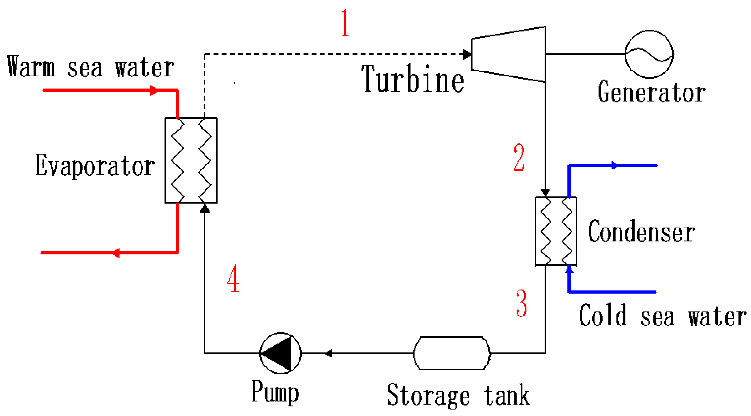
2.1.1. Mathematical Model of the OTEC

Ignoring the heat loss in the heat exchange process of the heat exchanger [21], the energy conservation equation of the evaporator and condenser is:

$${\mathrm{m}}_4(h_1-h_4)={\mathrm{m}}_w{\mathrm{c}}_w(T_{wi}-T_{w\mathrm{o}}),$$

(1)

$${\mathrm{m}}_2(h_2-h_3)={\mathrm{m}}_c{\mathrm{c}}_c(T_{ci}-T_{co}),$$

(2)

where m is mass flow rate, kg/s, h is enthalpy, kJ/kg, c is specific heat capacity, kJ/(kg·K), T is temperature, K. Subscript 1 to 4 are state points, Subscript w is warm sea water and c is cold sea water. Subscript i and o are inlet and outlet.

The thermodynamic process of the working fluid in the turbine is an isentropic expansion process [22], and its output power is

$${\mathrm{W}}_T={\mathrm{m}}_1(h_1-h_2)$$

(3)

The thermodynamic process of the working fluid in the pump is an adiabatic compression process, and the power consumption of the pump is

$${\mathrm{W}}_p={\mathrm{m}}_3(h_4-h_3),$$

(4)

The net power output of the ocean thermal energy conversion system is calculated as follows:

$${\mathrm{W}}_{net}={\mathrm{W}}_T-{\mathrm{W}}_p,$$

(5)

The theoretical efficiency of the cycle is

$${\mathsf{\eta }}_0=\frac{(h_1-h_2)-h_4-h_3}{h_1-h_4},$$

(6)

2.1.2. Parameters of Thermoelectric Power Generation System

This article uses warm sea water as the heat source of the organic Rankine cycle. According to the 2016 South China Sea Environmental Status Bulletin issued by the South China Sea Branch of the State Oceanic Administration in June 2017, the South China Sea temperature fluctuates between 24.6 °C and 30.1 °C.

From May to October, the surface water temperature of the South China Sea can be maintained above 28 °C for a total of 6 months. Therefore, this paper selects 28 °C as the heat source temperature. The temperature of deep cold sea water is generally stable, and the cold source temperature is set at 4 °C.

Studies have shown [23] that the temperature difference between the inlet and outlet of seawater in the heat exchanger is about 2~4 °C. When the temperature difference of seawater in the heat exchanger becomes smaller, it has a huge impact on the power consumption of the pump. When the temperature change of warm sea water and cold sea water in the heat exchanger is greater than 2 °C, the power consumption of the warm sea water and cold sea water pump will be maintained at a low level, so the temperature drop of the warm sea water and the temperature rise of the cold sea water are 2 °C. According to the reference [24,25,26], the pitch point temperature of the evaporator and condenser is 2 °C.

The choice of circulating working fluid should not only consider its theoretical thermodynamic properties, but also fully consider safety and environmental friendliness. In this study, the refrigerant R134a was selected as the working fluid of the turbine [27] based on the research of Sauret and Rowlands, which evaluated five different fluids based on the QGECE (Queensland Geothermal Energy Center of Excellence) thermodynamic model. Results showed that the highest performance cycle based on R134a generates 33% higher net power than the lowest performance cycle based on n-pentane [28,29,30,31]. In addition, R134a has relatively low critical pressure and temperature, low flammability, low toxicity and relative inertness. Also, impact on the environment is relatively small; namely, low global warming potential (global warming potential) and low ozone depletion potential (ozone depletion potential).

According to the international authoritative working fluid physical property database (NIST REFPROP V9.1) [32] developed by the National Institute of Standards and Technology (NIST), the physical property parameters of each state point are calculated, as shown in

Table 1. State point parameters of ocean thermal energy conversion system.

State Point	Temperature T/K	Pressure P/Mpa	Density ρ/(Kg/m3)	Enthalpy h/(kJ/kg)	Entropy s/(kJ/kg·K)
1(Turbine inlet)	297.15	0.6400	31.049	411.98	1.7177
2′(Turbine outlet)	281.15	0.3876	19.084	401.70	1.7177
2(Condenser inlet)	281.20	0.3876	18.933	403.24	1.7232
3(Condenser outlet)	281.15	0.3876	1267.9	210.84	1.0388
4(Evaporator inlet)	297.15	0.6400	1268.6	211.03	1.0388

. The design conditions of the turbine can also be obtained in

Table 2. Turbine design parameters and requirements.

Parameter	Value
Total pressure of inlet p1/MPa	0.64
Total temperature of inlet T1/K	297.15
Static pressure of outlet p2/MPa	0.38761
Mass flow rate $\mathrm{m}$/kg·s−1	3.82
Isentropic efficiency ηs/–	0.85

.

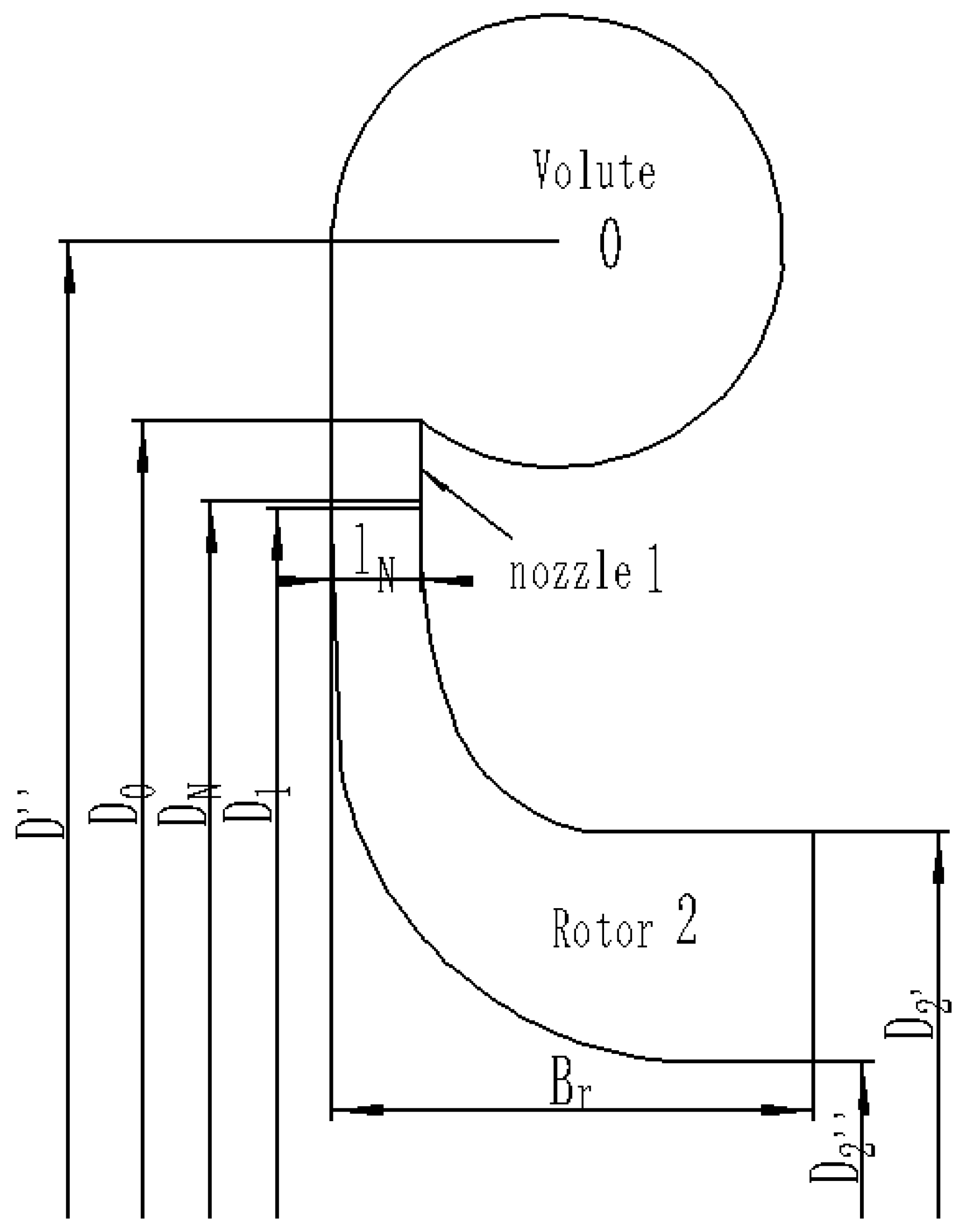
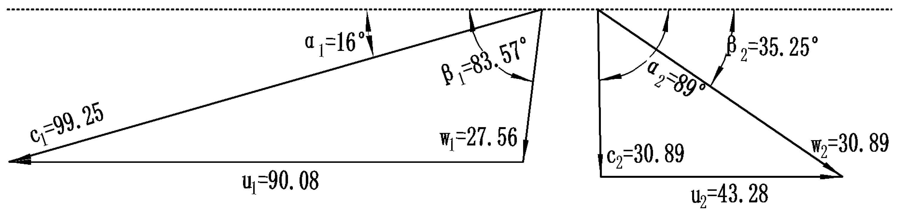
2.2. One-Dimensional Design of Radial-Inflow Turbine for ORC

Aiming at the application characteristics of marine thermal energy conversion in a small temperature difference environment and the special thermophysical properties of the organic working fluid in this environment, the aerodynamic design and optimization of this turbine are carried out combined with the design ideas of ORC radial turbine [33,34]. The overall working process of the centripetal turbine is shown in Figure 2. Firstly, working gas flows into the volute at a certain speed which is evenly distributed to the nozzle vanes; then, the gas enters the nozzle to expand, making part of the internal energy convert into kinetic energy (0–1), of which the pressure decreases, the temperature decreases and the speed rises. Next, the gas accelerated by the nozzle enters the rotor at high speed to push the rotor to rotate, driving the motor to generate electricity, while the gas continues to expand in the rotor, completing the internal energy to mechanical energy transition (1–2). Finally, the working fluid flows out of the turbine to the pipeline after passing through the diffuser.

2.2.1. Initial Parameter Optimization

The preliminary design of the centripetal turbine takes 50% of the engineering time, which is due to too many empirical parameters being used in the preliminary design of the turbine [35]. The first step of one-dimensional design is to determine the basic parameters, because the use of different basic parameters will lead to a large number of design solutions with different geometric dimensions and losses. According to the energy equation and the velocity triangle, the wheel efficiency of the radial turbine is given by Equation (7):

$$\begin{gathered} {\mathsf{\eta }}_u=2{\overline{u}}_1[\phi \cos \alpha 1\sqrt{1-\Omega }-{\overline{D}}_2{}^2{\overline{u}}_1+ \\ {\overline{D}}_2\psi \cos {\beta }_2\sqrt{\Omega +{\phi }^2\left(1-\Omega \right)+{\overline{D}}_2{}^2{\overline{u}}_1{}^2-2{\overline{u}}_1\phi \cos \alpha 1\sqrt{1-\Omega }}, \end{gathered}$$

(7)

Turbine circumference efficiency is determined by 7 basic parameters; namely, reaction degree Ω, wheel diameter ratio ${\overline{D}}_2$, speed ratio ${\overline{u}}_1$ and nozzle speed coefficient φ, rotor speed coefficient ψ, rotor inlet absolute airflow angle α₁ and outlet relative flow angle β_2.

These seven basic parameters are first selected by the method of genetic algorithm optimization with the goal of maximizing wheel efficiency [36]. At the same time, they are corrected to meet the corresponding flow channel requirements during the calculation process. The final values and empirical ranges of the 7 basic parameters [37] are shown in

Table 3. The basic parameters and results.

Basic Parameters	Design Result	Reference Range
Ω	0.49	0.35–0.55
${\overline{D}}_2$	0.47	0.3–0.5
${\overline{u}}_1$	0.636	0.65–0.7
φ	0.96	0.95–0.97
ψ	0.84	0.75–0.85
α1/°	16	12–30
β2/°	35.25	20–45

.

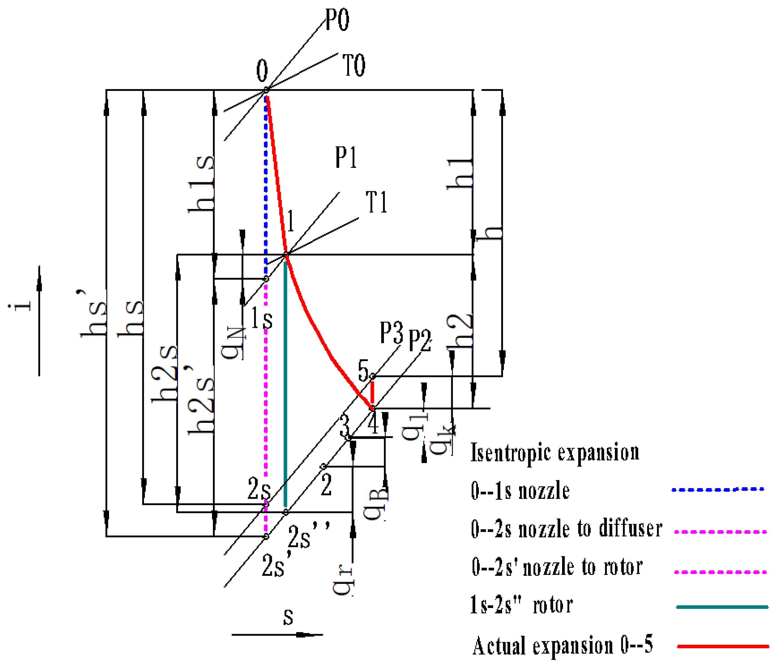
2.2.2. Mathematical Model

In the process of one-dimensional initial design and thermal calculation of the turbine, the internal flow can usually be regarded as a steady-state flow that ignores the temperature change of specific heat and isentropic exponent, adiabatic and inviscid [38]. The gas first expands and accelerates in the nozzle, which increases the gas velocity at the nozzle outlet to $C_1$. Then, the gas rotates into the rotor at a high relative speed of ${\mathsf{\omega }}_1$. The circumferential velocity of the blade is $u_1$, and the gas continues to expand in the blade. The relative velocity of the airflow in the outlet is called ${\mathsf{\omega }}_2$, and its absolute velocity $C_2$ is the vector sum of the velocities $u_2$ and ${\mathsf{\omega }}_2$ at this point.

The rotor inlet circumferential velocity, absolute velocity, relative velocity and relative flow angle are given by:

$$u_1={\overline{u}}_1{C}_S,$$

(8)

$$C_1=\mathsf{\psi }\sqrt{2(1-\Omega )h_{s^{\prime }}},$$

(9)

$${\mathsf{\omega }}_1=\frac{C_1\sin {\alpha }_1}{\sin {\beta }_1},$$

(10)

$$\tan {\beta }_1=\frac{\sin {\alpha }_1}{\cos {\alpha }_1-\frac{u_1}{C_1}},$$

(11)

where $C_S$ is the ideal velocity of the flow at rotor outlet and isentropic ideal enthalpy drop $h_{s^{\prime }}$ has the form

$$C_S=\sqrt{2h_{s^{\prime }}},$$

(12)

$$h_{s^{\prime }}=i_0-i_{2s^{\prime }},$$

(13)

The relative velocity, absolute velocity, peripheral velocity and relative flow angle at the rotor outlet are calculated as:

$${\mathsf{\omega }}_2=\sqrt{2h_{2s}+{\mathsf{\omega }}_1{}^2+u_{2m}{}^2-u_1{}^2},$$

(14)

$$C_2=\frac{{\mathsf{\omega }}_{2\sin {\beta }_2}}{\sin {\alpha }_2}$$

(15)

$$u_2=\mathsf{\mu }{u}_1$$

(16)

$$\tan {\alpha }_2=\frac{\sin {\beta }_2}{\cos {\beta }_2-\frac{u_{2m}}{{\mathsf{\omega }}_{2^{\prime }}}}$$

(17)

The gas flow conditions in the inlet and exhaust of the rotor are represented by velocity triangles at the inlet and outlet of the rotor, as shown in Figure 3.

The thermal parameters of the internal runner part of the turbine are calculated accordingly based on the determination of the basic parameters, and the main design dimensions and structure of the runner including the volute, the nozzle and the rotor are obtained. The rotor inlet diameter is given by:

$$D_1=\sqrt{\frac{\dot{m}}{\pi \left(\frac{l_1}{D_1}\right){\mathsf{\omega }}_1\sin {\beta }_1{\rho }_1{\tau }_1}},$$

(18)

where $l_1$ and ${\tau }_1$ are respectively the rotor blade height and the rotor blockage factor at the inlet, $\frac{l_1}{D_1}$ is specified as 0.04 by experience.

The nozzle outlet diameter is calculated as:

$$D_N=D_1+2{\Delta }_1,$$

(19)

where ${\Delta }_1$ is the length of the interspace between the nozzle and rotor, set as 1 mm.

The nozzle blade height is given by:

$$l_N=\frac{\dot{m}}{{\rho }_1{C}_1\pi D_N{\tau }_N\sin {\alpha }_1^{\prime }},$$

(20)

where ${\tau }_N$ is the nozzle outlet blockage factor.

The rotor blade height at the inlet has the form

$$l_1=l_N+\Delta l,$$

(21)

$$\Delta l=1.7{\Delta }_1$$

(22)

In Equations (23) and (24), $D_{2^{\prime }}$ and $D_{2^{″}}$ denote the shroud diameter and hub diameter at the rotor outlet, respectively.

$$D_{2^{\prime }}=\sqrt{D_{2m}{}^2+\frac{2A_2}{\pi {\tau }_2}},$$

(23)

$$D_{2^{″}}=\sqrt{D_{2m}{}^2-\frac{2A_2}{\pi {\tau }_2}}$$

(24)

where $A_2$ is the rotor outlet area and $D_{2m}$ is the average diameter of the rotor outlet, defined as

$$A_2=\frac{\dot{m}}{{\mathsf{\omega }}_2\sin {\beta }_2{\rho }_2},$$

(25)

$$D_{2m}={\overline{D}}_2{D}_1,$$

(26)

The rotor blade height at the outlet has the form

$$l_2=\frac{1}{2}\left({\mathrm{D}}_{2^{\prime }}-{\mathrm{D}}_{2^{″}}\right),$$

(27)

Considerable spread angle of working wheel midday [39]

$$\mathsf{\theta }={\tan }^{-1}\frac{2\left(l_2-l_1\right)}{D_1-D_{2m}},$$

(28)

The rotational speed is given by

$$\mathrm{n}=\frac{60u_1}{\pi D_1},$$

(29)

Radial turbine isentropic expansion efficiency

$${\mathsf{\eta }}_{s^{\prime }}=\frac{ \mathrm{h}}{h_s}=\frac{ i_0-i_4}{i_0-i_{2s^{\prime }}},$$

(30)

$$W_T={\mathsf{\eta }}_s{h}_s\mathrm{m}$$

(31)

Among them, h is the actual enthalpy drop of the turbine,$i_0$ is the enthalpy value of the turbine inlet, respectively, $i_4$ and $i_{2s^{\prime }}$ are the actual enthalpy value and isentropic enthalpy value of the diffuser outlet, respectively.

In the process of gas expansion, certain losses will inevitably occur. In order to improve design accuracy, it is necessary to consider the energy loss $q_N$ in the nozzle, the energy loss $q_r$ in the rotor, the energy loss $q_k$ of the diffuser in the turbine calculation unit wheel back friction loss $q_B$ and internal leakage loss $q_l$.

$$q_N=\left(1-{\mathsf{\psi }}^2\right)h_{1s},$$

(32)

$$q_r=\frac{1}{2}\left({\mathsf{\omega }}_{2s^{\prime }}{}^2-{\mathsf{\omega }}_{2^{\prime }}{}^2\right),$$

(33)

$$q_k=\frac{1}{2}\left(C_{2^{\prime }}{}^2-C_{3^{\prime }}{}^2\right),$$

(34)

$$q_B=\frac{4{\xi }_f{\rho }_1{u}_1{}^3{D}_1{}^2}{\mathrm{m}},$$

(35)

where ${\xi }_f$ is the friction coefficient of the rotor

When $\frac{\delta }{l_m}\le 0.05$,

$$q_l=1.3\frac{\delta }{l_m}\left(h_{s^{\prime }}-q_N-q_r-q_B\right),$$

(36)

When $\frac{\delta }{l_m}>0.05$

$$q_l=(0.05+0.31\frac{\delta }{l_m})\left(h_{s^{\prime }}-q_N-q_r-q_B\right)$$

(37)

$$l_m=\frac{l_1+l_2}{2},$$

(38)

$\frac{\delta }{l_m}$ is the relative axial clearance of the working wheel

The flow channel efficiency of a radial turbine can be calculated by Formula (39).

$${\mathsf{\eta }}_{s^{\prime }}=1-\left({\xi }_N+{\xi }_r+{\xi }_k+{\xi }_B+{\xi }_l\right),$$

(39)

Here,${\xi }_i=\frac{q_i}{h_s}$, $i$ is a different subscript code.

2.2.3. Design Results and Verification

The main aerodynamic design parameters of the radial inflow turbine can be obtained, according to the above-mentioned initial design parameters and one-dimensional model, as shown in

Table 4. 1-D thermal design results.

Parameter	Design Result
Nozzle outlet blockage factor ${\tau }_{\mathrm{N}}$	0.98
Rotor inlet blockage factor ${\tau }_1$	0.965
Rotor outlet blockage factor ${\tau }_2$	0.775
Relative axial clearance of rotor $\frac{\delta }{l_m}$	0.017
wheel back friction coefficient of rotor ${\xi }_f$	0.00042
Rotation speed N/r·min–1	7993
Output power WT/kW	33.04
Isentropic efficiency ηs/–	0.8574
Diameter of nozzle inlet $D_0/\mathrm{mm}$	222
Diameter of nozzle onlet $D_N/\mathrm{mm}$	300
Height of nozzle inlet $l_N$/mm	8.48
Number of nozzle blade ZN	32
Absolute airflow angle of rotor inlet α1/°	16
Relative airflow angle of rotor inlet β1/°	83.05
Circumferential speed of rotor inlet u1/m·s–1	92.077
Absolute speed of rotor inlet c1/m·s–1	99.25
Relative speed of rotor inlet ω1/m·s–1	27.56
Diameter of rotor inlet D1/mm	220
Height of rotor inlet l1/mm	10.18
Absolute airflow angle of rotor outlet α2/°	89
Absolute airflow angle of rotor outlet β2/°	35.25
Circumferential speed of rotor outlet u2/m·s–1	43.27
Absolute speed of rotor outlet c2/m·s–1	30.89
Relative speed of rotor outlet ω2/m·s–1	53.52
Absolute airflow angle of rotor outlet α2/°	73.19
Outer diameter of rotor outlet D2′/mm	127
Inner diameter of rotor outlet D2″/mm	71
Height of rotor outlet $l_2/\mathrm{mm}$	28
Axial length of rotor Br$/\mathrm{mm}$	65
Number of rotor blade (Zr)	14

. The Enthalpy-entropy change of the working fluid in the calculation process is shown in Figure 4, which details the change of the thermodynamic parameters of the entire expansion process. The actual fluid properties refer to NISTREFPROP 9.1.

In order to ensure the accuracy of the one-dimensional calculation, the design results are verified based on the data provided by the references. The comparison between the results of this study and the references is shown in

Table 5. Verification of design result.

Basic Parameters	Design Result	Reference Range
$\mathsf{\theta }$	17.06	<20° [39]
$\frac{D_N}{D_0}$	1.36	1.1–1.7 [40]
$\frac{{\mathrm{D}}_{2^{\prime }}}{D_1}$	0.58	<0.7 [41]
$\frac{{\mathrm{D}}_{2^{″}}}{{\mathrm{D}}_1}$	0.32	0.2~0.3 [42]

. It can be seen that the design results of this study are all within the range given in the references, and are in good agreement with them.

2.3. Three-Dimensional Numerical Simulations of the Radial-Inflow Turbine for OTEC

In order to compare between the one-dimensional calculation results and the CFD results, ANSYS-CFX was selected to perform steady-state 3D viscous flow simulation. As a professional software (ANSYS 2019 R1, 31/12/2020) for turbomachinery simulation, this commercial software (ANSYS 2019 R1, 31/12/2020) has certain reliability. For the sake of robustness and the experience gained from previous CFD work, the first-order upwind convection scheme is used to realize the discretization of the Reynolds averaged Navier-Stokes (RANS) equation, and the $\mathrm{k}$-$\mathsf{\epsilon }$- turbulence model with a scalable wall function is selected, which is simple, stable, saves computing resources, and is widely used in the fields of aviation and turbomachinery [43,44]. In addition, it is solved by general equations (energy, momentum, mass) provided by ANSYS-CFX.

2.3.1. Theoretical Model

(1) Reynolds Averaged Navier-Stokes (RANS) Equations

As described above, turbulence models seek to solve a modified set of transport equations by introducing averaged and fluctuating components. For example, a velocity $U_i$ may be divided into an average component,${\overline{U}}_i$, and a time varying component,$u_{i }$.

$$U_i={\overline{U}}_i+u_i$$

(40)

$${\overline{U}}_i=\frac{1}{\mathsf{\Delta }t}\underset{t}{\overset{\mathrm{t}+\mathsf{\Delta }t}{{\displaystyle \int }}}{U}_{i}dt$$

(41)

Substituting the averaged quantities into the original transport equations results in the Reynolds averaged equations given below.

$$\frac{\partial \mathsf{\rho }}{\partial \mathrm{t}}+\frac{\partial }{\partial x_j}\left(\rho U_j\right)=0$$

(42)

$$\frac{\partial \mathsf{\rho }{U}_i}{\partial \mathrm{t}}+\frac{\partial }{\partial x_j}\left(\rho U_i{U}_j\right)=-\frac{\partial p}{\partial x_i}+\frac{\partial }{\partial x_j}\left({\tau }_{ij}-\rho \overline{u_i{u}_j}\right)+S_M$$

(43)

The Reynolds averaged energy equation is:

$$\begin{gathered} \frac{\partial \mathsf{\rho }{h}_{tot}}{\partial \mathrm{t}}-\frac{\partial \mathrm{p}}{\partial \mathrm{t}}+\frac{\partial }{\partial x_j}\left(\rho U_j{h}_{tot}\right) \\ =\frac{\partial }{\partial x_j}\left(\lambda \frac{\partial T}{\partial x_j}-\rho \overline{u_{j}h}\right)+\frac{\partial }{\partial x_j}\left[U_i\left({\tau }_{ij}-\rho \overline{u_i{u}_j}\right)\right]+S_E \end{gathered}$$

(44)

The mean Total Enthalpy is given by:

$$h_{tot}=h+\frac{1}{2}{U}_i{U}_i+\frac{1}{2}\overline{u_i{}^2}$$

(45)

Similarly, the Additional Variable $\mathsf{\varphi }$ may be divided into an average component,$\overline{\mathsf{\varphi }}$, and a time varying component, $\mathsf{\phi }$. After dropping the bar for averaged quantities, except for products of fluctuating quantities, the Additional Variable equation becomes

$$\frac{\partial \mathsf{\rho }\mathsf{\varphi }}{\partial \mathrm{t}}+\frac{\partial }{\partial x_j}\left(\rho U_j\mathsf{\varphi }\right)=\frac{\partial }{\partial x_j}\left(\Gamma \frac{\partial \mathsf{\varphi }}{\partial x_j}-\rho \overline{u_j\mathsf{\phi }}\right)+S_{\mathsf{\varphi }}$$

(46)

where $\mathsf{\Delta }t$ is a time scale that is large in relation to the turbulent fluctuations, but small in relation to the time scale to which the equations are solved; $\tau$ is the molecular stress tensor (including both normal and shear components of the stress); the $\rho \overline{u_i{u}_j}$, $\rho \overline{u_{j}h }$ and $\rho \overline{u_i\mathsf{\phi }}$ are the Reynolds flux terms; the $\frac{\partial }{\partial x_j}\left[U_i\left({\tau }_{ij}-\rho \overline{u_i{u}_j}\right)\right]$ term in the equation is the viscous work term; $S_M$ and $S_E$ are momentum source and energy source; $\Gamma$ is diffusivity

(2) The k-Epsilon Model

$\mathrm{k}$ is the turbulence kinetic energy and is defined as the variance of the fluctuations in velocity. It has dimensions of (L² T⁻²); for example, m²/s². $\mathsf{\epsilon }$ is the turbulence eddy dissipation (the rate at which the velocity fluctuations dissipate), and has dimensions of per unit time (L² T⁻³); for example, m²/s³.

The $\mathrm{k}$-$\mathsf{\epsilon }$ model introduces two new variables into the system of equations. The continuity equation is then:

$$\frac{\partial \mathsf{\rho }}{\partial \mathrm{t}}+\frac{\partial }{\partial x_j}\left(\rho U_j\right)=0$$

(47)

And the momentum equation becomes:

$$\frac{\partial \mathsf{\rho }{U}_i}{\partial \mathrm{t}}+\frac{\partial }{\partial x_j}\left(\rho U_i{U}_j\right)=-\frac{\partial p^{\prime }}{\partial x_i}+\frac{\partial }{\partial x_j}\left[{\mu }_{eff}\left(\frac{\partial U_i}{\partial x_j}+\frac{\partial U_j}{\partial x_i}\right)\right]+S_M$$

(48)

$$p^{\prime }=p+\frac{2}{3}\rho k+\frac{2}{3}{\mu }_{eff}\frac{\partial U_k}{\partial x_k}$$

(49)

$${\mu }_{eff}=\mu +{\mu }_t$$

(50)

$${\mu }_t=C_{\mu }\mathsf{\rho }\frac{{\mathrm{k}}^2}{\mathsf{\epsilon }}$$

(51)

The values of $\mathrm{k}$ and $\mathsf{\epsilon }$ come directly from the differential transport equations for the turbulence kinetic energy and turbulence dissipation rate:

$$\frac{\partial \left(\mathsf{\rho }k\right)}{\partial \mathrm{t}}+\frac{\partial }{\partial x_j}\left(\rho U_{j}k\right)=\frac{\partial }{\partial x_j}\left[\left(\mu +\frac{{\mu }_t}{{\sigma }_k}\right)\frac{\partial k}{\partial x_j}\right]+P_k-\rho \epsilon +P_{kb}$$

(52)

$$\frac{\partial \left(\mathsf{\rho }\epsilon \right)}{\partial \mathrm{t}}+\frac{\partial }{\partial x_j}\left(\rho U_j\epsilon \right)=\frac{\partial }{\partial x_j}\left[\left(\mu +\frac{{\mu }_t}{{\sigma }_{\epsilon }}\right)\frac{\partial \epsilon }{\partial x_j}\right]+\frac{\epsilon }{k}(C_{\epsilon 1}{P}_k-C_{\epsilon 2}\rho \epsilon +C_{\epsilon 1}{P}_{\epsilon b})$$

(53)

$$P_k={\mu }_t\left(\frac{\partial U_i}{\partial x_j}+\frac{\partial U_j}{\partial x_i}\right)\frac{\partial U_i}{\partial x_j}-\frac{2}{3}\frac{\partial U_k}{\partial x_k}\left(3{\mu }_t\frac{\partial U_k}{\partial x_k}+\mathsf{\rho }k\right)$$

(54)

where $S_M$ is the sum of body forces, ${\mu }_{eff}$ is the effective viscosity accounting for turbulence, $C_{\mu }=0.09,$ $C_{\epsilon 1}=1.14$,$C_{\epsilon 2}=1.92$, ${\sigma }_k=1.0$ and ${\sigma }_{\epsilon }=1.3$ are constants, $P_{kb}$ and $P_{\epsilon b}$ represent the influence of the buoyancy forces.

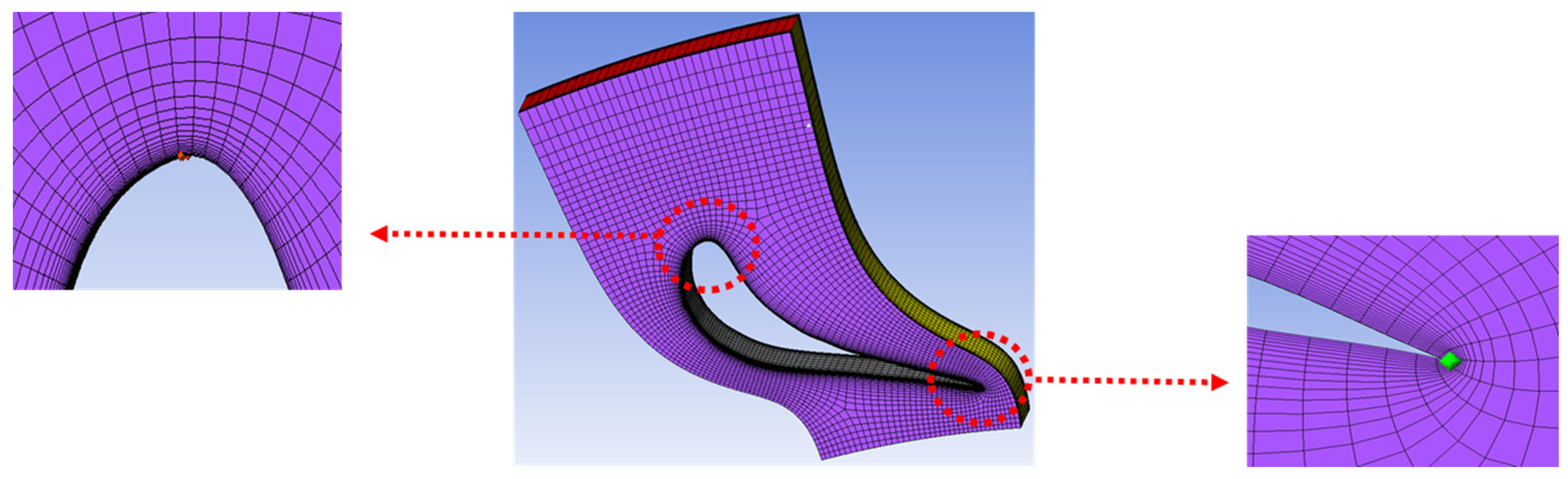
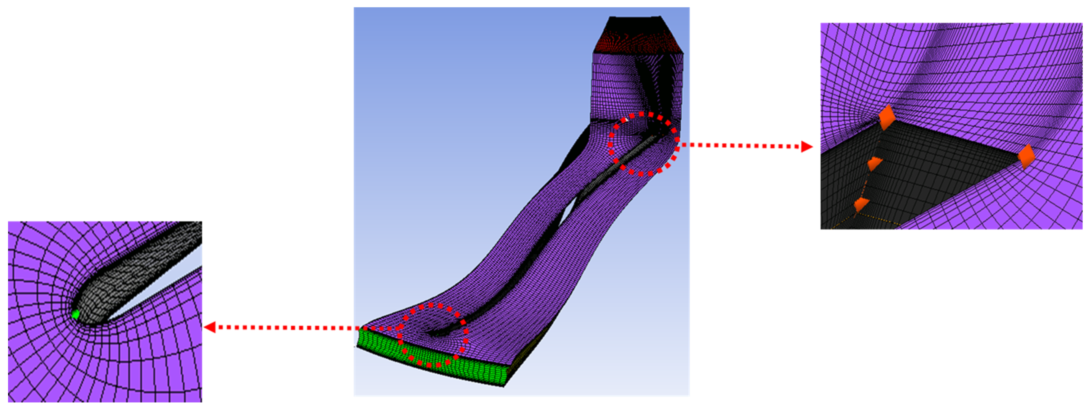
2.3.2. 3D Modeling and Meshing

The geometry of the turbine is exported to ANSYS-BladeGen to generate the nozzle and rotor channels. Ansys-TurboGrid is used to generate O-H three-dimensional computational grids, as shown in Figure 5 and Figure 6, where the “automatic topology and meshing (ATM optimization)” option is used in the stator and rotor flow channels. It can generate high-quality grids and avoid negative volumes, which is a problem for traditional grid generation [45]. The volute is divided into a tetrahedral mesh, and the volute tongue is locally encrypted. The overall mesh after importing into CFX is shown in Figure 7. This initial mesh was found good enough to run pioneering simulations of the 3D candidate R134a radial-inflow turbine in high flow conditions and establish the complete methodology (thermodynamic cycle, meanline analysis and preliminary viscous CFD simulations).

The properties of the refrigerant R134a in the radial-inflow turbine is described by the equation of state (EoS) of Peng-Robinson which is same to the equation of Sauret and Gu [46]. Peng-Robinson EoS provided by ANSYS-CFX is not also simplicity, but also accuracy of this model to perform preliminary real gas compuational simulations. And the EoS also has reasonable accuracy, especially near the critical point [47]. The equations are given as:

$$\mathrm{p}=\frac{RT}{V_m-b}-\frac{\mathrm{a}\alpha }{V_m{}^2+2b{V}_m-b^2},$$

(55)

$$\mathrm{a}=\frac{0.457235R^2{T}_c{}^2}{p_c}$$

(56)

$$\mathrm{b}=\frac{0.077796R{T}_c{}^2}{p_c},$$

(57)

$$\alpha ={\left(1+к\left(1-T_r^{0.5}\right)\right)}^2,$$

(58)

$$\mathsf{\kappa }=0.37464+1.54226\mathsf{\omega }-0.26992{\mathsf{\omega }}^2,$$

(59)

$$T_r=\frac{T}{T_c},$$

(60)

where $\mathsf{\omega }$= 0.326 is the acentric factor of refrigerant R134a,$T_c=374.26 \mathrm{K}$ and $p_c= 4059 \mathrm{kPa}$ are, respectively, the critical temperature and pressure of R134a, $V_m$ is the molar volume and $R$ is the universal gas constant.

To complete the description of the real gas properties, the CFD solver calculates the enthalpy and the entropy using relationships which are detailed in [48]. These relationships depend on the zero pressure ideal gas specific heat capacity ${\mathrm{c}}_{{\mathrm{p}}_0}$ and the derivatives of the Peng–Robinson EoS. ${\mathrm{c}}_{{\mathrm{p}}_0}$ is obtained by a fourth-order polynomial whose coefficients are defined by Poling et al. [49].

2.3.3. Boundary Condition Setting and Simulation Monitoring

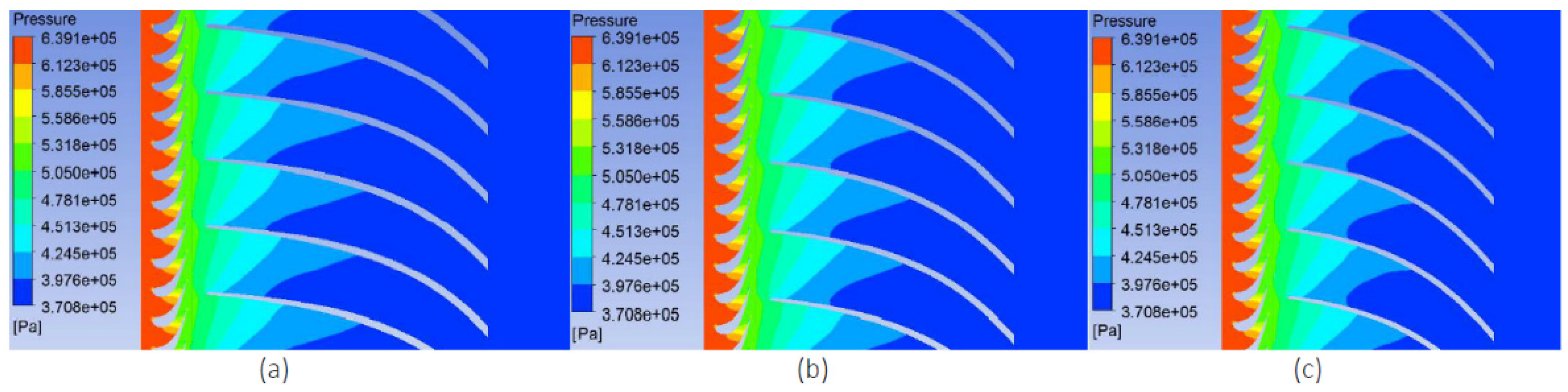
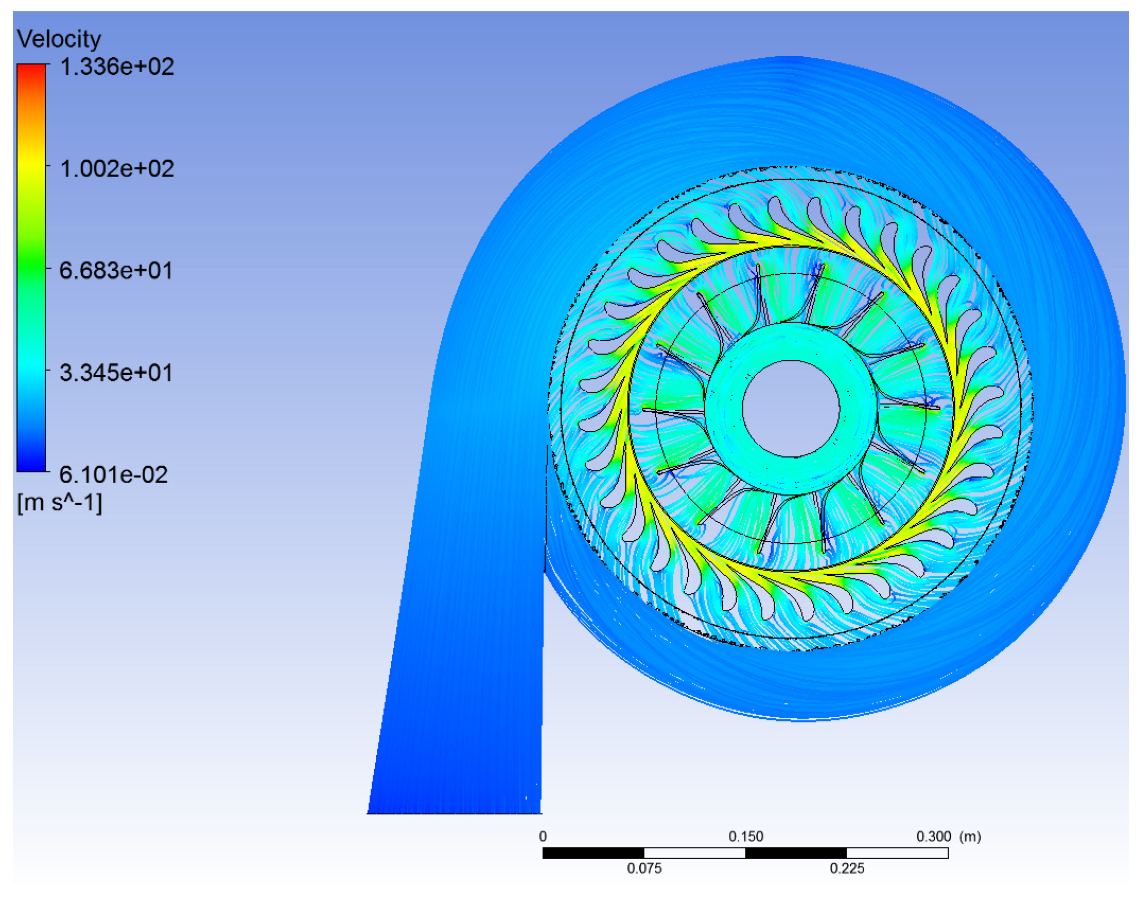
The initial simulation and optimization process uses pressure inlet and mass flow outlet as the inlet and outlet conditions, and monitors the outlet pressure and isentropic expansion efficiency. When verifying the optimization results, the pressure inlet and pressure outlet boundary conditions are used and the inlet and outlet mass flow and isentropic expansion efficiency are monitored. The specific boundary conditions are listed below:

1. The rated speed of the rotor is defined from the preliminary design and set to 7993 rpm (Table 4).

2. The inlet of the volute is set as the pressure inlet, total pressure (0.64 MPa) and total temperature (297.15 K); the diffuser outlet is set as the mass flow outlet, and the mass flow (3.82 kg/s) is calculated from the cycle (Table 2).

3. There are two interfaces between the outlet of the stator and the inlet of the rotor and between the outlet of the rotor and the inlet of the diffuser, both of which are dynamic connections, defined as the Frozen-rotor model; The volute outlet to the stator inlet is static connection, defined as Stage-Frame Change/Mixing and Automatic Pitch Change model.

3. Results

Figure 8 shows the pressure distribution of the radial turbine for different blade heights. The pressure decreases from the inlet to the outlet of the turbine. For each blade height, the pressure distribution of the nozzle channel is very uniform, and the pressure changes are mainly concentrated in the outlet part where the isobars are dense. The pressure surface and the suction surface are basically symmetrical, and there is no pressure sudden change and reverse pressure gradient. For the rotor channel, the isobars at the front are dense and the pressure gradient is large. Most of the pressure drop is caused by the expansion of the working fluid. On the whole, the pressure changes are relatively uniform and the pressure gradient is relatively slow. On the pressure surface side, the pressure changes slowly and the high pressure area is larger due to the gas impact. It can be seen from the figure that the suction surface pressure is lower than the pressure surface at the same position. In fact, this corresponds to the working principle of the rotor. The gas expanding in the nozzle and entering the rotor will push the rotor to do work, while the gas continues to expand in the rotor, further increasing the driving force on the rotor. The acting surfaces of these forces are pressure surfaces, so the pressure of the pressure surface is higher than the suction surface.

Figure 9 and Figure 10 are the overall turbine streamline diagram and the streamline distribution at 50% leaf height, respectively. In order to better show the streamlines, the diffuser in Figure 9 is not shown. It can be seen from Figure 9 that the flow of the turbine from the volute to the stationary blade and then to the moving blade is good, and the streamline is relatively smooth and uniform along the direction of the flow channel, without obvious shock waves and reverse flow. Figure 10 shows the development of streamlines in the nozzle and the rotor. The velocity changes in the nozzle are mainly concentrated in the outlet section where the gas velocity reaches the maximum, and there is a uniform transition from the nozzle outlet to the rotor inlet without obvious shock waves. The distribution of streamlines in the rotor is relatively uniform, with only a slight speed jump on the suction surface, which is completely consistent with the pressure distribution law in Figure 8, and will not cause too much flow loss.

Table 6. Comparison of simulation results and design results.

Parameter	Design Result	Simulation Result	Relative Erro/%
Velocity of nozzle outlet c1/m·s−1	99.25	96.8827	2.39
Static pressure of turbine outlet p2/MPa	0.3876	0.3847	0.75
Reaction degree Ω	0.49	0.51	4.08
Isentropic efficiency ηs/%	85.74	88.66	3.41
Output Power P/kW	33.04	34.57	4.63

shows the comparison between numerical simulation results and aerodynamic design values under design conditions. It can be seen from Table 6 that the relative error of turbine nozzle outlet velocity, turbine outlet pressure, reaction degree, power and isentropic efficiency are all within a reasonable range (<5%), indicating that the simulation results are basically consistent with the one-dimensional design.

The nozzle outlet velocity and reaction degree represent the expansion state of the working fluid in the nozzle and the rotor, respectively. The higher the coincidence with the one-dimensional design value, the closer the working fluid in the nozzle and the rotor is to the ideal state, and the better the performance of the turbine. The outlet pressure is determined by the condenser in the cycle, which is an important evaluation factor in the turbine design process. The difference between the simulation value and the design value is small, indicating that the gas state at the outlet of the turbine outlet is close to the inlet of the condenser, which can avoid unnecessary pressure loss and ensure that the turbine can obtain the highest efficiency. Efficiency is an important indicator for evaluating the performance of a turbine and the output power determines the overall cycle output directly. In this simulation result, both of these two indicators exceed the design value, indicating that the overall performance of the turbine meets the design requirements, can obtain better energy output, and improve energy utilization.

4. Discussion

For further verification and analysis, the turbine outlet boundary is changed to the pressure outlet condition on the basis of the simulation in Section 2.3, keeping other conditions unchanged, and the inlet and outlet mass flow and efficiency are monitored for simulation. The results are shown in

Table 7. Comparative analysis of verification results.

Parameter	Design Result	Inlet and Outlet Boundary Conditions
		Pressure Inlet and Mass Flow Outlet	Pressure Inlet and Pressure Outlet
Velocity of Nozzle Outlet c1/m·s−1	99.25	96.8827	96.1358
Static pressure of turbine outlet p2/MPa	0.3876	0.3847	0.3876
Mass flow $\dot{m}$/kg·s−1	3.82	3.82	3.7953
Reaction degree Ω	0.49	0.51	0.5032
Isentropic efficiency ηs/%	85.74	88.66	89.9136
Output Power P/kW	33.04	34.57	34.6968

.

Mass flow is an important indicator for evaluating turbine design under the conditions of pressure inlet and pressure outlet, which given in the calculation of the entire ocean thermal energy conversion power generation cycle. The small difference between the simulation value and the design value indicates that the turbine has a high matching with the overall cycle, and the actual working process will be closer to the design conditions, which can ensure the highest efficiency under standard conditions. From the results given in Table 7, it can be seen that the mass flow rate of 3.79 kg/s has little difference from the design value, under the conditions of pressure inlet and pressure outlet.

In Table 7, “Pressure Inlet and Mass Flow Outlet” and “Pressure Inlet and Pressure Outlet” are two different inlet and outlet boundary conditions. “Pressure Inlet and Mass Flow Outlet” are pressure inlet (0.64 MPa) and mass flow outlet (3.83 kg/s); “Pressure Inlet and Pressure Outlet” are pressure inlet (0.64 MPa) and pressure outlet (0.3876 MPa). The performance of the turbine designed in this paper is verified by comparing the simulation results and design results under two different boundary conditions. At the same time, the two sets of simulation results can also be compared. The results show that the difference between simulation results and design results is very small, indicating that the performance of the turbine meets the design requirements. At the same time, the output power and efficiency in two sets of simulation are both higher than the design values, which are in good agreement with each other results, which can prove that the performance of this turbine under standard operating conditions can meet the design requirements.

5. Conclusions

This paper further completes the design process of the radial inflow turbine for ocean thermal energy conversion. The one-dimensional design and three-dimensional CFD analysis of the radial inflow turbine were carried out on the basis of parameter optimization of the ocean thermal energy conversion system. Under design conditions, the performance of the turbine is verified by changing the inlet and outlet conditions of the radial turbine. The main conclusions are summarized as follows.

(1) Three-dimensional CFD analysis shows that the turbine pressure distribution and streamline distribution are uniform without obvious backflow and vortex, at the same time, the nozzle and rotor are well coupled and the internal flow field is stable in the designed OTEC radial inflow turbine.

(2) The three-dimensional CFD simulation results are in good agreement with the one-dimensional design results, indicating that the design model proposed in this paper is reliable.

(3) Under different import and export conditions, the radial inflow turbine can achieve better power output and higher efficiency, indicating that the performance of this turbine under given standard conditions meets the application requirements of ocean thermal energy conversion.

References

1. Wei, D.; Lu, X.; Zhen, L.; Gu, J. Performance analysis and optimization of organic Rankine cycle (ORC) for waste heat recovery. Energy Convers. Manag. 2007, 48, 1113–1119. [Google Scholar] [CrossRef]
2. Koroneos, C.; Rovas, D. Exergy analysis of geothermal electricity using the Kalina cycle. Int. J. Exergy 2013, 12, 54–69. [Google Scholar] [CrossRef]
3. Binger, A. Potential and Future Prospects for Ocean Thermal Energy Conversion (OTEC) in Small Island Developing States (SIDS). Water Sci. Technol. 2004, 20, 88–90. [Google Scholar]
4. Al-Weshahi, M.A. Working fluid selection of low grade heat geothermal Organic Rankine Cycle (ORC). Int. J. Therm. Sci. 2014, 4, 6–12. [Google Scholar]
5. Imran, M.; Park, B.S.; Kim, H.J.; Lee, D.H.; Usman, M.; Heo, M. Thermo-economic optimization of Regenerative Organic Rankine Cycle for waste heat recovery applications. Energy Convers. Manag. 2014, 87, 107–118. [Google Scholar] [CrossRef]
6. Liu, W.M.; Chen, F.Y.; Wang, Y.Q.; Jiang, W.J.; Zhang, J.G. Progress of Closed-Cycle OTEC and Study of a New Cycle of OTEC. Adv. Mater. Res. 2012, 354–355, 275–278. [Google Scholar] [CrossRef]
7. Bao, J.; Zhao, L. A review of working fluid and expander selections for organic Rankine cycle. Renew. Sustain. Energy Rev. 2013, 24, 325–342. [Google Scholar] [CrossRef]
8. Whitfield, A. The Preliminary Design of Radial Inflow Turbines. J. Turbomach. 1990, 112, 50–57. [Google Scholar] [CrossRef]
9. Fiaschi, D.; Manfrida, G.; Maraschiello, F. Design and performance prediction of radial ORC turboexpanders. Appl. Energy 2015, 138, 517–532. [Google Scholar] [CrossRef]
10. Han, Z.; Fan, W.; Zhao, R. Improved thermodynamic design of organic radial-inflow turbine and ORC system thermal performance analysis. Energy Convers. Manag. 2017, 150, 259–268. [Google Scholar] [CrossRef]
11. Zhai, L.; Xu, G.; Wen, J.; Quan, Y.; Fu, J.; Wu, H.; Li, T. An improved modeling for low-grade organic Rankine cycle coupled with optimization design of radial-inflow turbine. Energy Convers. Manag. 2017, 153, 60–70. [Google Scholar] [CrossRef] [Green Version]
12. Wu, T.; Shao, L.; Wei, X.; Ma, X.; Zhang, G. Design and structure optimization of small-scale radial inflow turbine for organic Rankine cycle system. Energy Convers. Manag. 2019, 199, 111940. [Google Scholar] [CrossRef]
13. Flores, R.A.; Jiménez, H.M.A.; González, E.P.; Uribe, L.A.G. Aerothermodynamic design of 10kW radial inflow turbine for an organic flashing cycle using low-enthalpy resources. J. Clean. Prod. 2020, 251, 119713. [Google Scholar] [CrossRef]
14. Ithesh, K.G.; Chatterjee, D.; Oh, C.; Lee, Y.H. Design and performance analysis of radial-inflow turboexpander for OTEC application. Renew. Energy 2016, 85, 834–843. [Google Scholar] [CrossRef]
15. Nithesh, K.G.; Chatterjee, D. Numerical prediction of the performance of radial inflow turbine designed for ocean thermal energy conversion system. Appl. Energy 2016, 167, 1–16. [Google Scholar] [CrossRef]
16. Nithesh, K.G.; Samad, A. Integrated CFD-Surrogate optimization to enhance efficiency of turbine designed for OTEC. Main Themes 2016, 148. [Google Scholar]
17. Kim, D.Y.; Kim, Y.T. Design of a 100kW-class radial inflow turbine for ocean thermal energy conversion using R32. J. Korean Soc. Mar. Eng. 2014, 38, 1101–1105. [Google Scholar]
18. Kim, D.Y.; Kim, Y.T. Preliminary design and performance analysis of a radial inflow turbine for ocean thermal energy conversion. Renew. Energy 2017, 106, 255–263. [Google Scholar] [CrossRef]
19. Zhao, W.G. Research and Development of 200W Ammonia Saturated Steam Turbine for Experiment. Ph.D. Thesis, Tianjin University, Tianjin, China, 2005. [Google Scholar]
20. Ge, Y.Z.; Peng, J.P.; Wu, H.Y.; Chen, F.Y.; Liu, L.; Zhang, W.J. Aerodynamic design and performance study of a centripetal turbine with ocean temperature difference energy. Renew. Energy 2019, 37, 1560–1566. [Google Scholar]
21. Wang, Y.Q. Engineering Thermodynamics, 4th ed.; Higher Education Press: Beijing, China, 2007. [Google Scholar]
22. Zhu, Z.Q.; Wu, Y.T. Chemical Engineering Thermodynamics, 3rd ed.; Chemical Industry Press: Beijing, China, 2010. [Google Scholar]
23. Albert, S.; Kim, H.; Kim, J. Ocean Thermal Energy Conversion (OTEC): Past, Present, and Progress; IntechOpen: London, UK, 2020. [Google Scholar]
24. Chen, F.Y. Research on Thermal Performance and Comprehensive Utilization of Ocean Thermal Energy Power Generation Device. Ph.D. Thesis, Harbin Engineering University, Harbin, China, 2016. [Google Scholar]
25. Li, Y.C.; Liu, T.; Chen, X.X. Research on the best temperature difference of heat exchanger. New Energy 2000, 22, 10–13. [Google Scholar]
26. Wang, Y.Q. Research on the Shangyuan Cycle System for Ocean Thermal Power Generation. Ph.D. Thesis, Qingdao Technological University, Qingdao, China, 2011. [Google Scholar]
27. Sauret, E.; Rowlands, A.S. Candidate radial-inflow turbines and high-density working fluids for geothermal power systems. Energy 2011, 36, 4460–4467. [Google Scholar] [CrossRef]
28. Hettiarachchi, H.D.M.; Golubovic, M.; Worek, W.M. Optimum design criteria for an Organic Rankine cycle using low-temperature geothermal heat sources. Energy 2007, 32, 1698–1706. [Google Scholar] [CrossRef]
29. Marcuccilli, F.; Thiolet, D. Optimizing binary cycles with radial inflow turbines. Trans. Geotherm. Resour. Counc. 2009, 33, 737–743. [Google Scholar]
30. Hung, T.C.; Wang, S.K.; Kuo, C.H.; Pei, B.S.; Tsai, K.F. A study of organic working fluids on system efficiency of an ORC using low-grade energy sources. Energy 2010, 35, 1403–1411. [Google Scholar] [CrossRef]
31. Schuster, A.; Karellas, S.; Aumann, R. Efficiency optimization potential in supercritical Organic Rankine Cycles. Energy 2010, 35, 1033–1039. [Google Scholar] [CrossRef]
32. Higashi, Y. NIST Thermodynamic and Transport Properties of Refrigerants and Refrigerant Mixtures (REFPROP). NETSU Bussei 2000, 14, 1575–1577. [Google Scholar]
33. Li, Y.S. Non-developable straight-grained paraboloid and its application in the design of radial turbine wind deflector (final report). J. Shanghai Inst. Mach. 1980, 78–96. [Google Scholar]
34. Zheng, Y.; Hu, D.; Cao, Y.; Dai, Y. Preliminary design and off-design performance analysis of an Organic Rankine Cycle radial-inflow turbine based on mathematic method and CFD method. Appl. Therm. Eng. 2017, 112, 25–37. [Google Scholar] [CrossRef]
35. Aungier, R.H. Aerodynamic Performance Analysis of Axial-Flow Turbines; ASME Press: New York, NY, USA, 2006. [Google Scholar]
36. Song, P.; Sun, J.; Wang, K.; He, Z. Development of an Optimization Design Method for Turbomachinery by Incorporating the Cooperative Coevolution Genetic Algorithm and Adaptive Approximate Model. In Proceedings of the ASME 2011 Turbo Expo: Turbine Technical Conference and Exposition, Vancouver, BC, Canada, 6–10 June 2011. [Google Scholar]
37. Li, Y.; Lu, G. Centripetal Turbine and Centrifugal Compressor, 1st ed.; Machinery Industry Press: Beijing, China, 1992; pp. 110–132. [Google Scholar]
38. Bekiloglu, H.E.; Bedir, H.; Anlas, G. Multi-objective optimization of ORC parameters and selection of working fluid using preliminary radial inflow turbine design. Energy Convers. Manag. 2019, 183, 833–847. [Google Scholar] [CrossRef]
39. Ji, G.H. Turboexpander; China Machinery Industry Press: Beijing, China, 1982. [Google Scholar]
40. Stewart, W.L. Turbine Design and Application: Chapter 4, Blade Design; NASA: Washington, DC, USA, 1973.
41. Wasserbauer, C.A.; Glassman, A.J. Fortran Program for Predicting Off-design Performance of Radial-Inflow Turbines. 1975; pp. 1–57. Available online: https://ntrs.nasa.gov/citations/19750024045 (accessed on 1 March 2021).
42. Romagnoli, A.; Martinez-Botas, R. Performance prediction of a nozzled and nozzleless mixed-flow turbine in steady conditions. Int. J. Mech. Sci. 2011, 53, 557–574. [Google Scholar] [CrossRef]
43. Rocha, P.C.; Rocha, H.B.; Carneiro, F.M.; da Silva, M.V.; Bueno, A.V. k–ω SST (shear stress transport) turbulence model calibration: A case study on a small scale horizontal axis wind turbine. Energy 2014, 65, 412–418. [Google Scholar] [CrossRef]
44. Louda, P.; Sváček, P.; Fořt, J.; Fürst, J.; Halama, J.; Kozel, K. Numerical simulation of turbine cascade flow with blade-fluid heat exchange. Appl. Math. Comput. 2013, 219, 7206–7214. [Google Scholar] [CrossRef]
45. Odabaee, M.; Sauret, E.; Hooman, K. Computational fluid dynamics simulation and turbomachinery code validation of a high pressure ratio radial-inflow turbine. In Proceedings of the 10th International Conference on Heat Transfer, Fluid Mechanics and Thermodynamics (HEFAT2014), Orlando, FL, USA, 14–16 July 2014. [Google Scholar]
46. Sauret, E.; Gu, Y. Three-dimensional off-design numerical analysis of an organic Rankine cycle radial-inflow turbine. Appl. Energy 2014, 135, 202–211. [Google Scholar] [CrossRef] [Green Version]
47. Wang, L.S.; Gardeler], H.; Gmehling, J. The Performance of EOS Models in the Prediction of Vapor-Liquid Equilibria in Asymmetric Natural Gas Mixtures. Chin. J. Chem. Eng. 1998, 6, 29–37. [Google Scholar]
48. Ansys, C. ANSYS CFX-Solver Theory Guide; ANSYS CFX Release; ANSYS: Canonsburg, PA, USA, 2019; Volume 11, pp. 69–118. [Google Scholar]
49. Poling, B.E. The Properties of Gases and Liquids; McGraw-Hill: New York, NY, USA, 1977. [Google Scholar]
Figure 1. Schematic diagram of ocean thermal energy conversion cycle:1–4 are state points (See Table 1 for details).
Jmse 09 00287 g001
Figure 2. Schematic of the radial inflow turbine meridional view.
Jmse 09 00287 g002
Figure 3. Velocity triangles at rotor inlet and outlet.
Jmse 09 00287 g003
Figure 4. Enthalpy-entropy diagram of the turbine expansion.
Jmse 09 00287 g004
Figure 5. The mesh of nozzle.
Jmse 09 00287 g005
Figure 6. The mesh of rotor.
Jmse 09 00287 g006
Figure 7. The overall mesh of turbine.
Jmse 09 00287 g007
Figure 8. Pressure cloud diagram under different blade heights: (a) 25% of the blade height; (b) 50% of the blade height; (c) 75% of the blade height.
Jmse 09 00287 g008
Figure 9. Overall streamline diagram.
Jmse 09 00287 g009
Figure 10. Velocity distribution map at 50% blade height.
Jmse 09 00287 g010