
Adaptive Polynomials for the Vibration Analysis of an L-Type Beam Structure with a Free End


1
Departament of Naval Architecture and Ocean Engineering, Chosun University, Gwangju 61452, Korea
2
Structural Design Departament, Hyundai Samho Heavy Industries, Jeollanam-do 58462, Korea
*
Author to whom correspondence should be addressed.
J. Mar. Sci. Eng. 2021, 9(3), 300; https://0-doi-org.brum.beds.ac.uk/10.3390/jmse9030300
Submission received: 2 February 2021
/
Revised: 25 February 2021
/
Accepted: 5 March 2021
/
Published: 8 March 2021
(This article belongs to the Special Issue Hydrodynamic Design of Ships)
Abstract
:Vibration analysis using the component mode method has been less popular than before, since computers are powerful enough to solve complicated structures by a single large finite model. However, many structural engineers designing local structures on a ship still need simple tools to check anticipated vibration problems during their design work. Since most of local structures on a ship are simple enough to consist of several substructures, the component mode method could be of use as long as good, natural mode functions can be provided so that reasonable natural frequencies can be yielded. In this study, since mode polynomials based on static deflection of cantilever beams fail to work to cover the various configurations of L-type beams with a free end, two alternatives are suggested. One is based on more flexible mode functions—we call them adaptive polynomials. The other is a purely mathematical approach, which makes realistic mode functions unnecessary. Suggested alternatives yield very good numerical results.
1. Introduction
Two component mode methods are well-known: component mode synthesis, suggested by Hurty [1,2] and Craig [3,4], and the branch mode method, suggested by Hunn [5] and Gladwell [6].
The L-type beam structure with a free end studied here has been used for the explanation of the branch mode method, where normal modes of cantilevers, together with rigid mode, are suggested for generating branch modes [7].
Bhat suggested higher mode functions using orthogonal polynomials, and applied these mode functions for the free vibration analysis of a single plate with different boundary conditions [8].
Bourquin [9], Hou [10], Hintz [11], and Benfield [12] have studied the constraints at the junction of the connected structures.
Recent studies have focused on nonlinear mechanics. Pagani et al. explained that the natural frequency and mode shape can be changed significantly when the metal structure is subjected to large displacement and rotation under geometrical nonlinear conditions [13]. Carrera et al. developed the Lagrange formula, including cross-sectional deformation, in order to implement the vibration mode of the composite beam structure in the nonlinear region [14].
Furthermore, Carrera et al. developed a theory that can be solved by converting a three-dimensional model for large deformation of a structure into one dimension, which was developed and applied to the calculation [15].
Pagani and Carrera [16] introduced the unified formulation for geometric, nonlinear analysis of metal structures, and explained the formula for handling large displacements and rotations. In order to solve the geometric nonlinear problem of the plate, Pagani et al. [17] explained various nonlinear theories, and how these theories affect the nonlinear static behavior of thin-walled structures in the large displacement and rotation.
Alessandro et al. [18] introduced application of the fundamental model reduction techniques used in structural dynamics to flexible, multibody systems.
Park [19] suggested mode functions for L-type beam structures with fixed ends, where constraints at a junction are described using fixed and simple supported boundary conditions. An application of this mode function for plate structure has also been found [20].
As mentioned, if suitable mode functions are available, the component mode method can be a powerful tool for the free vibration analysis of simple local structures.
The purpose of this study is to provide powerful mode functions for the free vibration analysis of L-type beam structures, as shown in Figure 1, which can work for various length ratios (0. and are the lengths of the connected L-type beam in Figure 1.
Fundamental mode function, based on a fourth-order polynomial that satisfies four boundary conditions of a cantilever beam, failed to work for free vibration analysis of an L-type beam structure with a free end, although it describes deflections of a cantilever beam reasonably well. It is a reasonable guess that any mode functions that can describe well the deflections of substructures, which are cantilever beams, may not be able to describe deflections of the L-type beam structure with a free end.
New fundamental mode functions, using a second-order polynomial together with higher orthogonal mode functions, are suggested. These new mode functions have been found to be suitable for the free vibration analysis of L-type beam structures for various length ratios (0. This good performance is because of the fact that new mode functions based on lower-order polynomials are flexible enough to describe various shapes of deflections of varying length ratios. In this sense, these new polynomials can be named as adaptive polynomials.
In addition, a purely mathematical approach is suggested, where no efforts to describe meaningful mode functions are necessary. Instead, pure mathematical polynomials that only satisfy geometrical boundary conditions at a free end are used.
2. Problem Description and Mathematical Model
An L-type beam structure with a free end is shown in Figure 1:
Where = = , = = are assumed to be same for notational simplicity; m is mass per unit length of beam, and E and I are the Young’s modulus and moment of inertia, respectively.
and are coordinates of substructrues of L-type structures in Figure 1.
In addition, and are non-dimensionalized, such that , .
and are lateral deflections of the horizontal and vertical beam, respectively:
where are the generalized coordinates, and are corresponding mode functions to describe lateral deflections of beams A and B. is vertical displacement of beam B.
The method proposed by Bhat to generate higher orthogonal polynomials is as follows:
It can be shown that the polynomial satisfies the orthogonality condition:
The coefficients and are implemented using the orthogonal formula of the beam function:
Note that this polynomial only satisfies geometrical boundary conditions, although a fundamental polynomial can be chosen to satisfy natural boundary conditions.
Given mode functions, generalized mass is
and generalized stiffness (k) is
where, , , and , are generalized mass and generalized stiffness of substructures of L-type structure.
Applying displacement continuity (r1) at the junction results in the following:
Similarly, applying slope continuity (qn) yields,
The mass and stiffness matrices (MA and KA, respectively) using the suggested polynomials are shown in Equations (16) and (17):
and MB and KB can be expressed in a similar manner. Using the displacement and slope continuity in Equations (14) and (15) yields Equation (18):
where α is the ratio of length for the subcomponents (α = LB/LA):
3. FEM (Finite Element Method) Analysis
For comparison, FEM analysis was performed first. The eam properties used are shown in Table 1, and Figure 2 shows the L-type finite element method (FEM) model and geometric boundary conditions.
In Figure 2, m is mass per unit length of beam, E and I are Young’s modulus and moment of inertia, respectively.
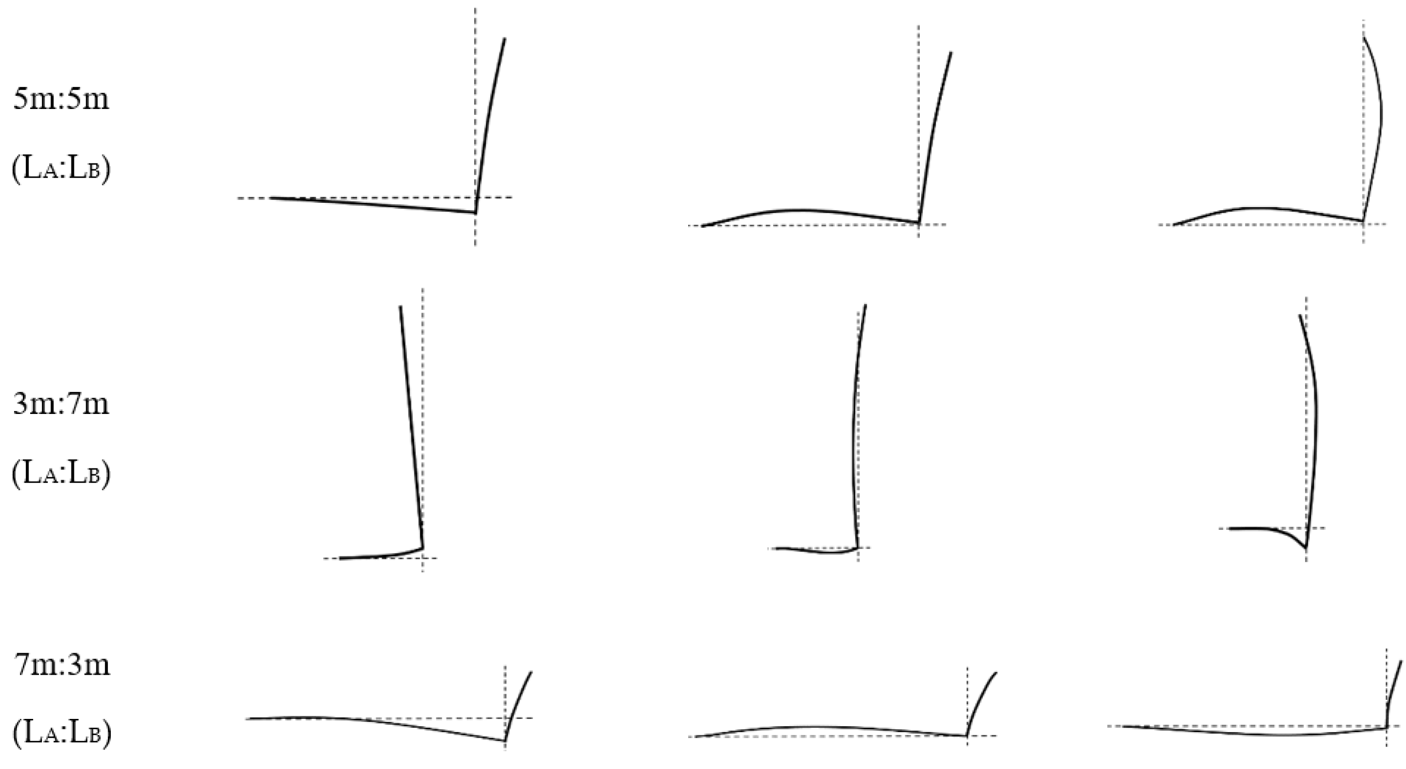
It is worth noting that the natural frequencies for the length ratio LB/LA are relatively similar to those for the length ratio LA/LB as like Figure 6, although mode shapes are different; this is somewhat interesting. However, it can be understood because this structure becomes a cantilever beam as LA or LB approaches zero.
4. Fundamental Mode Function Using Fourth-Order Polynomial and Numerical Results
The fourth-order polynomial for fundamental mode function can be easily obtained from four boundary conditions of a cantilever beam:
The lower four polynomials are shown in Table 2.
Free vibration analysis using these mode functions for a cantilever beam was performed.
5. Fundamental Mode Function Using Second-Order Polynomial (Adaptive Mode Function)
In order to make mode functions as flexible as possible, a second-order polynomial was chosen as a fundamental mode function, and higher orthogonal polynomials were generated, as suggested before by Bhat. In order to consider the rigid rotation of a vertical beam, is added.
The lower four mode functions are shown Table 4.
The numerical results are shown in Table 5, Table 6, Table 7. Thirteen mode functions, seven for and five for , were used for this numerical analysis.
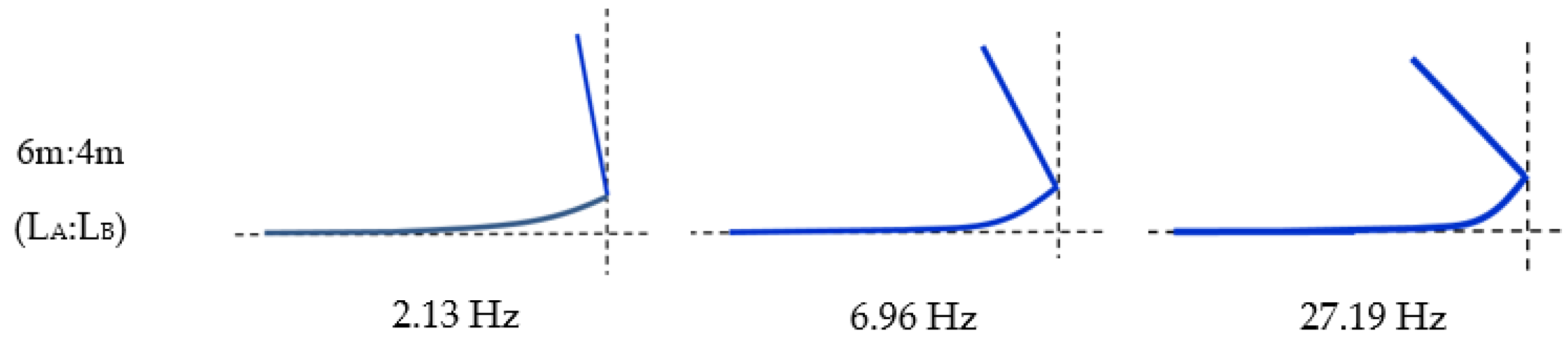
Typical corresponding natural modes are shown in Figure 9.
The numerical results showed very good agreement with the FEM results. This good agreement is due to the fact that suggested mode functions are flexible enough to follow anticipated deflections of an L-type beam with a free end. In that sense, we named these mode polynomials as having “adaptive mode function”.
6. Pure Mathematical Method
Mode functions for typical structures have been proposed, including this study [22,23]. There may be some structures where suitable mode functions may not be easy to generate.
In this case, a purely mathematical approach is suggested, where no meaningful higher-order mode functions are necessary. We may take mode functions in the following form:
Note that no higher-order mode functions are assumed. Most accurate natural frequencies are obtained using the how approach, although the eigenvectors obtained have no physical meaning.
This is due to the fact that no assumption for higher mode functions has been made. The numerical results were compared with those obtained from FEM analysis. Figure 1 was used for the calculation model and the beam properties mentioned in Table 1. The calculation results are shown in Table 8, Table 9, Table 10.
7. Discussion
Our work deals with a very classic subject, and little research based on the assumed mode method has been found in last 20 years. Furthermore, free vibration analysis of an L-type beam with a free end is a typical example, even in the textbooks, for explaining component mode synthesis.
However, we believe that our work can renew appreciation of the usefulness of component mode method for free vibration analysis, by providing powerful mode functions.
As you can see. it will not be an easy task to find mode functions that can work on various configurations of L-type beam structures (length ratio varies from 0 to ). Certain mode functions that can work for one specific value of may not work for different values of
Although we do not include it in the paper, the suggested mode function comes from dozens of candidates. If a component is divided into subcomponents which may have geometrical boundary conditions only at one end, like a cantilever, then free vibration solutions may be very sensitive to the choice of mode functions. Most methods based on the Rayleigh–Ritz method use assumed modes.
However, we suggest using pure mathematical functions instead of using an assumed mode function. Although mode shapes using mathematical functions have nothing to do with real mode shapes, the results of the proposed method are compared with the FEM results and shown in Table 5, Table 6, Table 7, Table 8, Table 9, Table 10.
As a result, the function is accurate enough to show an error rate of less than 2% in all sections, regardless of the length ratio of the connected structure.
8. Conclusions
A second-order fundamental polynomial, together with higher orthogonal polynomials, is suggested as the most suitable assumed mode functions for an L-type beam structure with a free end.
The robustness of the suggested polynomials is proven through numerical analysis for an L-type beam structure with a free end against varying length ratios.
A purely numerical approach has been suggested for the structures where substructures have geometrical conditions only at one end, like a cantilever beam.
The most accurate natural frequencies are obtained this way, since any assumptions for higher-mode functions are unnecessary. Once natural frequencies are obtained, the way to find corresponding natural modes is worth studing.
Author Contributions
Conceptualization, D.Y.Y., J.H.P.; methodology, D.Y.Y., J.H.P.; software, J.H.P.; validation, J.H.P., D.Y.Y.; formal analysis, J.H.P., D.Y.Y.; investigation, J.H.P.; writing—original draft preparation, J.H.P., D.Y.Y.; writing—review and editing, J.H.P., D.Y.Y.; funding acquisition. All authors have read and agreed to the published version of the manuscript.
Funding
This research has been supported by the Chosun University research fund.
Conflicts of Interest
The authors declare no conflict of interest.
References
- Hurty, W.C. Vibrations of structural systems by component mode synthesis. J. Eng. Mech. Div. 1960, 86, 51–70. [Google Scholar] [CrossRef]
- Hurty, W.C. Dynamic analysis of structural systems using component modes. AIAA J. 1965, 3, 678–685. [Google Scholar] [CrossRef]
- Craig, R.R.; Bampton, M.C.C. Coupling of sub-structures for dynamic analysis. AIAA J. 1968, 6, 1313–1319. [Google Scholar] [CrossRef] [Green Version]
- Craig, R.R.; Chang, C.J. A review of substructure coupling methods for dynamic analysis. Adv. Eng. Sci. 1976, 2, 393–408. [Google Scholar]
- Hunn, B.A. A method of calculating space free resonant modes of an aircraft. J. Roy. Aero. Soc. 1953, 57, 420. [Google Scholar] [CrossRef]
- Gladwell, G.M.L. Branch mode analysis of vibrating systems. J. Sound Vib. 1964, 1, 41–59. [Google Scholar] [CrossRef]
- Thorby, D. Structural Dynamics and Vibration in Practice, 1st ed.; Elsevier: London, UK, 2008; pp. 194–213. [Google Scholar]
- Bhat, R.B. Natural Frequencies of Rectangular Plates Using Characteristic Orthogonal Polynomials in Rayleigh-Ritz Method. J. Sound Vib. 1985, 102, 493–499. [Google Scholar] [CrossRef]
- Bourquin, F. Component mode synthesis and eigenvalues of second order operators: Discretization and algorithm. ESAIM Math. Model. Numer. Anal. 1992, 26, 385–423. [Google Scholar] [CrossRef] [Green Version]
- Hou, S. Review of modal synthesis techniques and a new approach. Shock Vib. Bull. 1969, 40, 25–39. [Google Scholar]
- Hintz, R.M. Analytical Methods in Component Modal Synthesis. AIAA J. 1975, 13, 1007–1016. [Google Scholar] [CrossRef]
- Benfield, W.A.; Hruda, R.F. Vibration Analysis of Structures by Component Mode Substitution. AIAA J. 1971, 9, 1255–1261. [Google Scholar] [CrossRef]
- Pagani, A.; Augello, R.; Carrera, E. Frequency and mode change in the large deflection and post-buckling of compact and thin-walled beams. J. Sound Vib. 2018, 432, 88–104. [Google Scholar] [CrossRef]
- Carrera, E.; Pagani, A.; Augello, R. Effect of large displacements on the linearized vibration of composite beams. Int. J. Non-linear Mech. 2020, 120, 103390. [Google Scholar] [CrossRef]
- Carrera, E.; Pagani, A.; Giusa, D.; Augello, R. Nonlinear analysis of thin-walled beams with highly deformable sections. Int. J. Non-Linear Mech. 2021, 128, 103613. [Google Scholar] [CrossRef]
- Carrera, E.; Pagani, A.; Augello, R. Evaluation of geometrically nonlinear effects due to large cross-sectional deformations of compact and shell-like structures. Mech. Adv. Mater. Struct. 2018, 27, 1269–1277. [Google Scholar] [CrossRef]
- Pagani, A.; Daneshkhah, E.; Xu, X.; Carrera, E. Evaluation of geometrically nonlinear terms in the large-deflection and post-buckling analysis of isotropic rectangular plates. Int. J. Non-Linear Mech. 2020, 121, 103461. [Google Scholar] [CrossRef]
- Alessandro, C.; Pappalardo, C. On the use of component mode synthesis methods for the model reduction of flexible multibody systems within the floating frame of reference formulation. Mech. Syst. Signal Process 2020, 142, 106745. [Google Scholar]
- Park, J.H.; Yoon, D.Y. A Proposal of Mode Polynomials for Efficient use of Component mode synthesis and Methodology to simplify the calculation of the connecting beams. J. Mar. Sci. Eng. 2021, 9, 20. [Google Scholar] [CrossRef]
- Park, J.-H.; Yang, J.-H. Normal Mode Analysis for Connected Plate Structure Using Efficient Mode Polynomials with Component Mode Synthesis. Appl. Sci. 2020, 10, 7717. [Google Scholar] [CrossRef]
- Thomson, W.T. Theory of Vibration with Applications, 4th ed.; Prentice Hall: Upper Saddle River, NJ, USA, 1993; pp. 360–365. [Google Scholar]
- Han, S.Y.; Huh, Y.C. Vibration Analysis of Quadrangular plate having attachments by the Assumed Mode Method. Trans. Soc. Nav. Archit. Korea 1995, 32, 116–125. (In Korean) [Google Scholar]
- Rubin, S. Improved component-mode representation for structural dynamic analysis. AIAA J. 1975, 13, 995–1006. [Google Scholar] [CrossRef]
Figure 1.
Simplified model of one end of a supported structure.

Figure 2.
L-type beam structure with a free end.

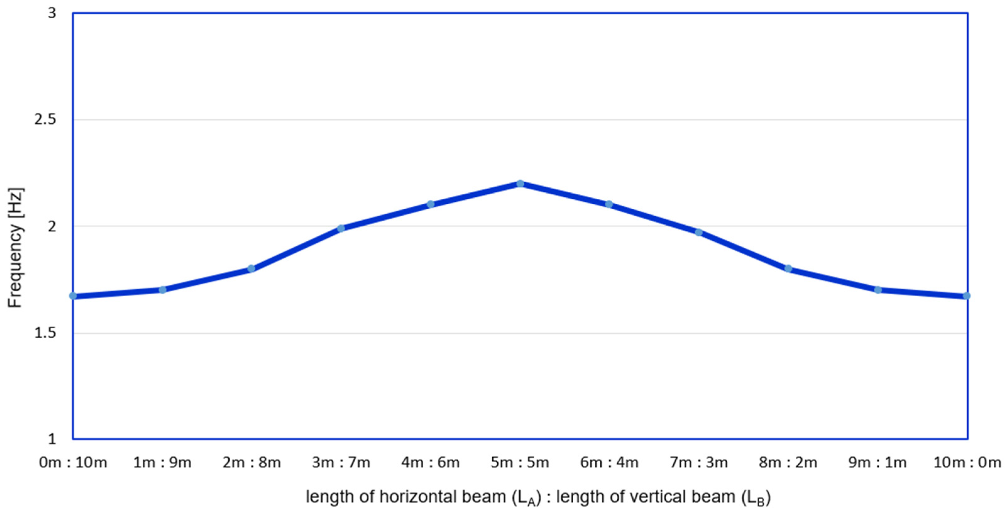
Figure 3.
Natural frequency of the first mode for an L-type beam structure.

Figure 4.
Natural frequency of the second mode for an L-type beam structure.

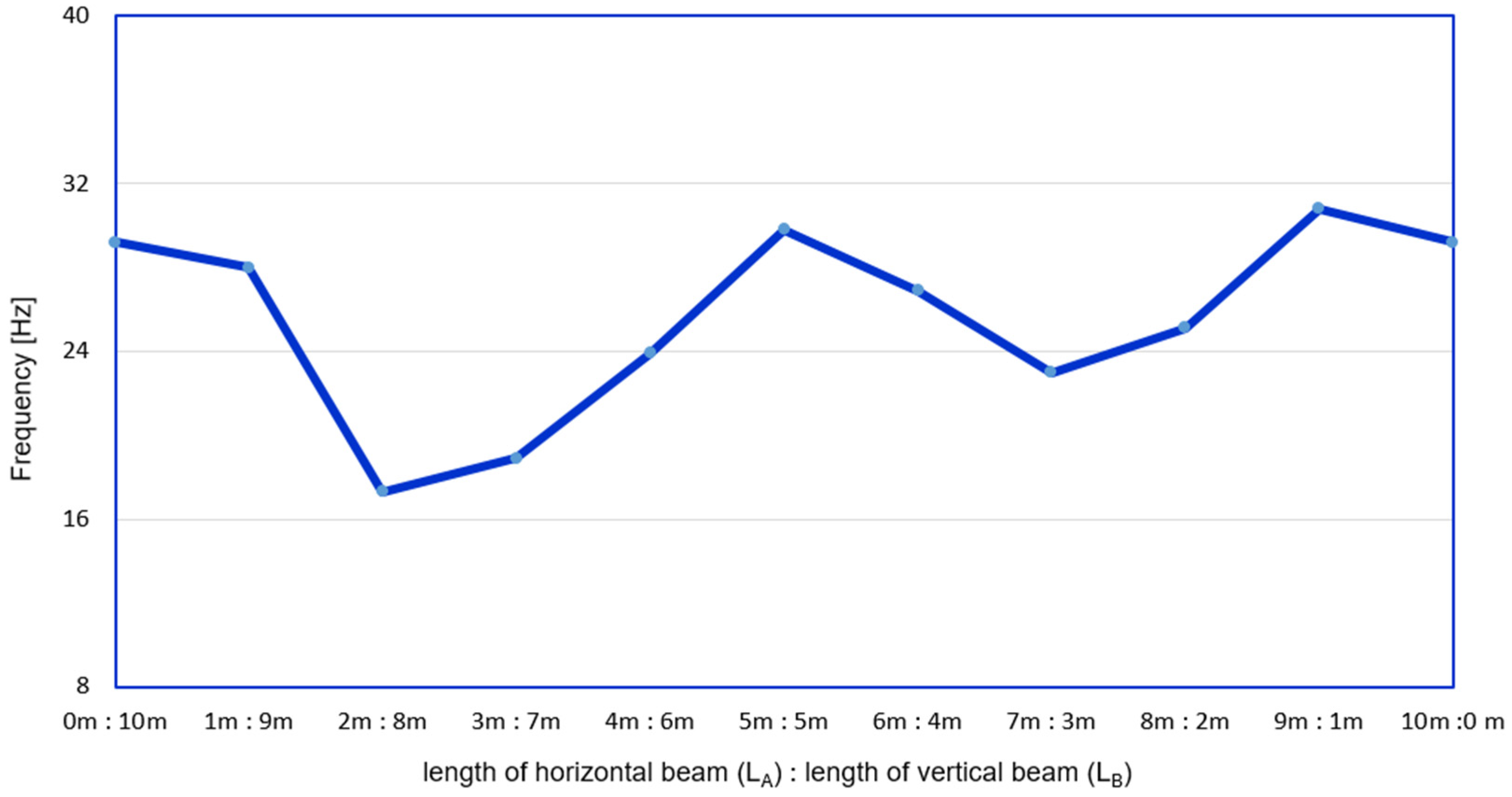
Figure 5.
Natural frequency of the third mode for an L-type beam structure.

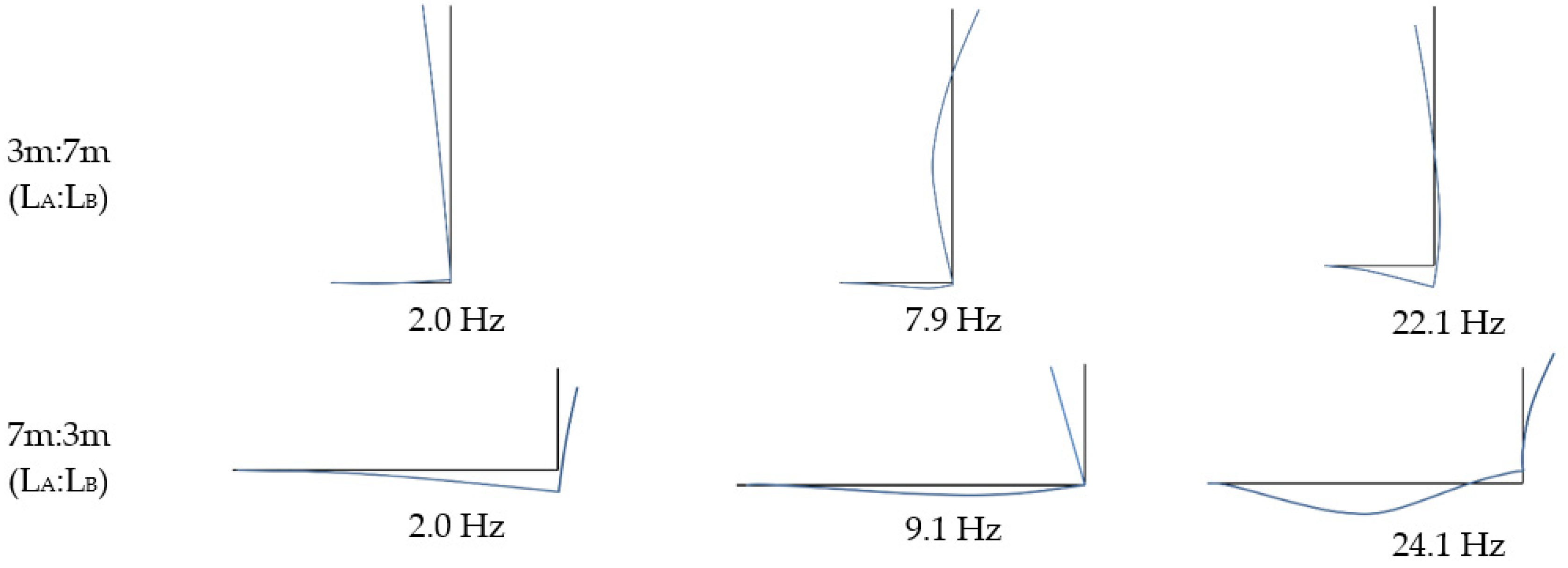
Figure 6.
Typical mode shape of FEM result: first, second, and third mode.

Figure 7.
The comparison result of FEM and an L-type connected beam (using a fourth-order polynomial): First mode.
Figure 7.
The comparison result of FEM and an L-type connected beam (using a fourth-order polynomial): First mode.

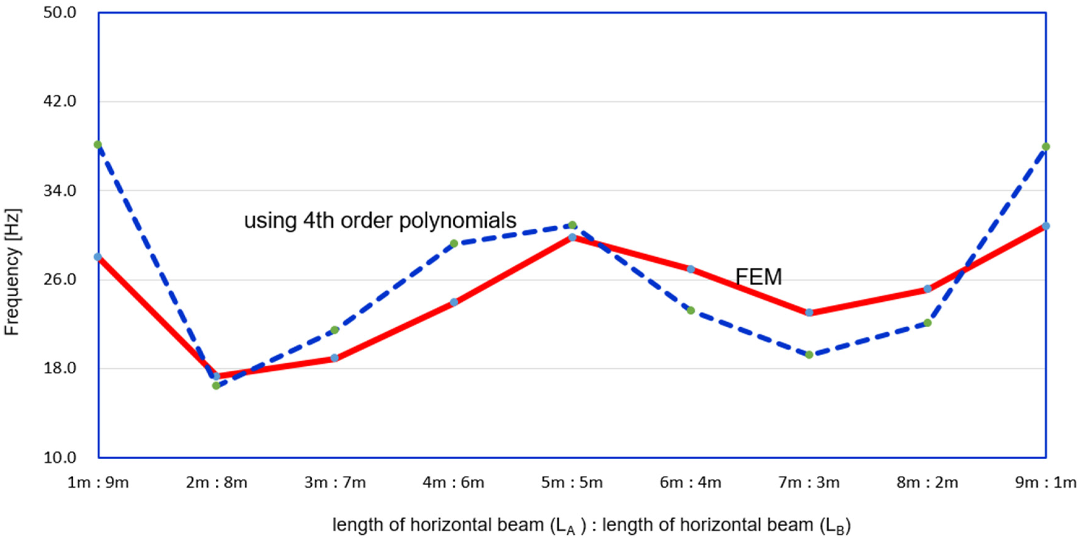
Figure 8.
The comparison result of FEM and an L-type connected beam (using a fourth-order polynomial): Third mode.
Figure 8.
The comparison result of FEM and an L-type connected beam (using a fourth-order polynomial): Third mode.

Figure 9.
The mode shape of using adaptive polynomials.

Figure 10.
Mode shapes using mathematical function.


Table 1.
Properties of the finite element method (FEM) model.
| Property | Cross Section | |
|---|---|---|
| Density (kg/m3) | 7850 |  |
| Total Length (LA + LB) (m) | 10 | |
| Young’s modulus (N/mm2) | 2.1 × 10⁵ | |
| Moment of inertia (mm4) | 3.33 × 10⁸ |
Table 2.
The mode function using fourth-order polynomial.
| i | |
|---|---|
| 1 | |
| 2 | |
| 3 | |
| 4 |
Table 3.
Comparison of FEM result and using a fourth-order polynomial.
| Fundamental | Remark | |||
|---|---|---|---|---|
| FEM result | 3.51 | 21.99 | 61.44 | |
| Using fourth-order polynomial | 3.51 | 22.00 | 61.70 |
Table 4.
The mode function using adaptive polynomials.
| i and j | ||
|---|---|---|
| 1 | ||
| 2 | ||
| 3 | ||
| 4 |
Table 5.
Comparison of FEM results and using adaptive polynomials: First mode.
| Length (LA:LB) | 0:10 | 1:9 | 2:8 | 3:7 | 4:6 | 5:5 | 6:4 | 7:3 | 8:2 | 9:1 | 10:0 |
| FEM | 1.67 | 1.70 | 1.80 | 1.99 | 2.10 | 2.20 | 2.10 | 1.97 | 1.80 | 1.70 | 1.67 |
| Adaptive polynomial | 1.67 | 1.71 | 1.82 | 2.00 | 2.10 | 2.20 | 2.10 | 1.97 | 1.80 | 1.71 | 1.67 |
Table 6.
Comparison of FEM results and using adaptive polynomials: second mode.
| Length (LA:LB) | 0:10 | 1:9 | 2:8 | 3:7 | 4:6 | 5:5 | 6:4 | 7:3 | 8:2 | 9:1 | 10:0 |
| FEM | 10.45 | 11.10 | 10.70 | 7.80 | 6.30 | 6.10 | 7.00 | 9.10 | 11.30 | 11.10 | 10.45 |
| Adaptive polynomial | 10.45 | 11.10 | 10.75 | 7.87 | 6.30 | 6.10 | 6.96 | 9.10 | 11.30 | 11.10 | 10.45 |
Table 7.
Comparison of FEM results and using adaptive polynomials: third mode.
| Length (LA:LB) | 0:10 | 1:9 | 2:8 | 3:7 | 4:6 | 5:5 | 6:4 | 7:3 | 8:2 | 9:1 | 10:0 |
| FEM | 29.20 | 28.00 | 17.30 | 18.90 | 23.90 | 29.80 | 26.90 | 23.00 | 25.10 | 30.80 | 29.20 |
| Adaptive polynomial | 29.20 | 28.90 | 17.40 | 19.00 | 24.12 | 29.80 | 27.00 | 23.20 | 25.40 | 31.50 | 29.20 |
Table 8.
Comparison of FEM results and using mathematical function: First mode.
| Length (LA:LB) | 0:10 | 1:9 | 2:8 | 3:7 | 4:6 | 5:5 | 6:4 | 7:3 | 8:2 | 9:1 | 10:0 |
| FEM | 1.67 | 1.70 | 1.80 | 1.99 | 2.10 | 2.20 | 2.10 | 1.97 | 1.80 | 1.70 | 1.67 |
| Mathematical function | 1.67 | 1.71 | 1.82 | 1.99 | 2.10 | 2.20 | 2.10 | 1.97 | 1.82 | 1.71 | 1.67 |
Table 9.
Comparison of FEM results and using mathematical function: Second mode.
| Length (LA:LB) | 0:10 | 1:9 | 2:8 | 3:7 | 4:6 | 5:5 | 6:4 | 7:3 | 8:2 | 9:1 | 10:0 |
| FEM | 10.45 | 11.10 | 10.70 | 7.80 | 6.30 | 6.10 | 7.00 | 9.10 | 11.30 | 11.10 | 10.45 |
| Mathematical function | 10.45 | 11.16 | 10.75 | 7.87 | 6.34 | 6.08 | 6.96 | 9.10 | 11.33 | 11.15 | 10.45 |
Table 10.
Comparison of FEM results and using mathematical function: Third mode.
| Length (LA:LB) | 0:10 | 1:9 | 2:8 | 3:7 | 4:6 | 5:5 | 6:4 | 7:3 | 8:2 | 9:1 | 10:0 |
| FEM | 29.20 | 28.00 | 17.30 | 18.90 | 23.90 | 29.80 | 26.90 | 23.00 | 25.10 | 30.80 | 29.20 |
| Mathematical function | 29.20 | 28.40 | 17.48 | 19.11 | 24.12 | 30.00 | 27.19 | 23.31 | 25.47 | 31.50 | 29.20 |
Table 11.
Eigenvectors of the mode shape.
| Coordinate | 2.1 Hz | 6.96 Hz | 27.2 Hz | Coordinate | 2.1 Hz | 6.96 Hz | 27.2 Hz |
|---|---|---|---|---|---|---|---|
| P1 ( | 1.00 | 1.00 | 1.00 | P11 ( | 2.23 | 26.60 | −15.65 |
| P2 ( | 1.10 | 3.78 | 2.65 | P12 ( | 2.36 | 29.07 | −18.33 |
| P3 ( | 1.22 | 6.45 | 2.36 | P13 ( | 2.49 | 31.54 | −21.04 |
| P4 ( | 1.34 | 9.05 | 1.08 | P14 ( | 2.62 | 34.00 | −23.75 |
| P5 ( | 1.46 | 11.61 | −0.75 | P15 ( | 2.76 | 36.47 | −26.48 |
| P6 ( | 1.58 | 14.14 | −2.91 | P16 ( | 2.89 | 38.93 | −29.23 |
| P7 ( | 1.71 | 16.65 | −5.28 | P17 ( | 3.02 | 41.39 | −31.99 |
| P8 ( | 1.84 | 19.15 | −7.78 | P18 ( | 3.16 | 43.84 | −34.77 |
| P9 ( | 1.97 | 21.64 | −10.36 | P19 ( | 3.29 | 46.30 | −37.57 |
| P10 ( | 2.10 | 24.12 | −12.99 | P20 ( | 3.42 | 48.75 | −40.39 |
Publisher’s Note: MDPI stays neutral with regard to jurisdictional claims in published maps and institutional affiliations. |
© 2021 by the authors. Licensee MDPI, Basel, Switzerland. This article is an open access article distributed under the terms and conditions of the Creative Commons Attribution (CC BY) license (http://creativecommons.org/licenses/by/4.0/).
Share and Cite
MDPI and ACS Style
Yoon, D.Y.; Park, J.H. Adaptive Polynomials for the Vibration Analysis of an L-Type Beam Structure with a Free End. J. Mar. Sci. Eng. 2021, 9, 300. https://0-doi-org.brum.beds.ac.uk/10.3390/jmse9030300
AMA Style
Yoon DY, Park JH. Adaptive Polynomials for the Vibration Analysis of an L-Type Beam Structure with a Free End. Journal of Marine Science and Engineering. 2021; 9(3):300. https://0-doi-org.brum.beds.ac.uk/10.3390/jmse9030300
Chicago/Turabian StyleYoon, Duck Young, and Jeong Hee Park. 2021. "Adaptive Polynomials for the Vibration Analysis of an L-Type Beam Structure with a Free End" Journal of Marine Science and Engineering 9, no. 3: 300. https://0-doi-org.brum.beds.ac.uk/10.3390/jmse9030300
Note that from the first issue of 2016, this journal uses article numbers instead of page numbers. See further details here.