3-Dimensional Modeling and Attitude Control of Multi-Joint Autonomous Underwater Vehicles

Abstract

To achieve rapid and flexible vertical profile exploration of deep-sea hybrid structures, a multi-joint autonomous underwater vehicle (MJ-AUV) with orthogonal joints was designed. This paper focuses on the 3-dimensional (3D) modeling and attitude control of the designed vehicle. Considering the situation of gravity and buoyancy imbalance, a 3D model of the MJ-AUV was established according to Newton’s second law and torque balance principle. And then the numerical simulation was carried out to verify the credibility of the model. To solve the problems that the pitch and yaw attitude of the MJ-AUV are coupled and the disturbance is unknown, a linear quadratic regulator (LQR) decoupling control method based on a linear extended state observer (LESO) was proposed. The system was decoupled into pitch and yaw subsystems, treated the internal forces and external disturbances of each subsystem as total disturbances, and estimated the total disturbances with LESO. The control law was divided into two parts. The first part was the total disturbance compensator, while the second part was the linear state feedback controller. The simulation results show that the overshoot of the controlled system in the dynamic process is nearly 0 rad, reaching the design value very smoothly. Moreover, when the controlled system is in a stable state, the control precision is within 0.005%.

1. Introduction

Ocean exploration technology is one of the difficult problems in frontier science and engineering in the ocean field. The deep-sea region hybrid is an important factor in maintaining global energy balance and driving deep ocean circulation. Therefore, it is of great strategic significance to use advanced technology to explore the deep-sea region hybrid structures [1]. The complex structure of the seabed, as well as unknown extreme fluid systems such as cold springs and hydrothermal fluids, make the work of exploration more difficult.

Most of the existing deep-sea submersibles struggle to meet the capabilities necessary to explore deep-sea hybrid structures rapidly. The glider [2,3] achieves pose control by adjusting the remaining buoyancy and the position of the mass center, but its motion trajectory is jagged and single, speed is slow, and maneuverability is poor. Most autonomous underwater vehicles (AUVs) [4] are rigid single-body structures and use tail rudder and attitude adjustment systems to control the movement direction. In order to further improve the ability of flexible steering of the AUV to allow rapid observation of the deep-sea 3-dimensional (3D) environment, a multi-joint AUV (MJ-AUV) was designed. It consists of three parts in series: diversion cabin, navigation/control cabin, and propulsion cabin, each of which is connected by a pair of orthogonal joints. In addition, its tail is equipped with a propeller. To adjust the yaw attitude and pitch attitude of the body, the MJ-AUV can change the hydrodynamic appearance of the vehicle by rotating the joints.

The MJ-AUV is a multi-rigid-body rootless system with high nonlinear and strong coupling characteristics, the kinematic and dynamic modeling of which is the basis of studying its motion behavior characteristics and control problems. Xia et al. [5] established a horizontal dynamic model of a fish-like robot based on Kane’s method. Aiming at the structure of the underwater gliding snake-like robot, Tang et al. [6] built a gliding and serpentine swimming model based on the momentum theorem, moment of momentum theorem, and recursive Newton–Euler method. Based on the principle of force and moment balance, Kelasidi et al. [7,8,9] built a horizontal plane and slope dynamics model of the underwater snake robot in the inertial system. In addition, the Euler–Lagrange method [10] and the Schiehlen method [11] have also been used to deal with multi-rigid body modeling.

The controller design is the key technology to enable underwater vehicles to complete a deep-sea exploration mission. Professor Pettersen’s team from the University of Norway has made many contributions in the field of underwater multi-joint robot control, such as planar path tracking in the presence of ocean currents [12] and integral line-of-sight guidance for path following control [13]. Fischer et al. [14] propose an error controller using continuous robust integration to compensate for the uncertainty of the AUV model and have carried out experiments under controlled and open-water environments to verify the effectiveness of the controller. Zhao et al. [15] propose an adaptive plus disturbance observer (DOB) controller for depth and attitude control of the AUV. The controller consists of DOB as an inner-loop compensator and a non-regressor based adaptive controller as an outer-loop controller. In addition, the experiments verify that the controller has strong robustness. Wu et al. [16], Wang et al. [17] and Kang et al. [18] make improvements on the basis of the adaptive controller, which is verified in the field of motion control of AUVs. Zhang et al. [19] present a sliding mode variable structure control algorithm, and simulation results show that this algorithm has advantages of high control accuracy and strong robustness. Rodriguez et al. [20] combine sliding mode control with adaptive control and propose a sliding mode adaptive controller, which is compared with non-adaptive control and PD control to verify the effectiveness of the controller. References [21,22,23,24,25] have made improvements based on the active disturbance rejection controller, combining sliding mode controller, self-searching optimal algorithm, or other methods, to improve the accuracy and anti-interference performance of the AUV motion control. In addition to the above methods, in recent years, scholars are also studying the application of reinforcement learning [26,27] and artificial intelligence algorithms [28] in the field of AUV control.

MJ-AUV is a complex system with high nonlinear, strong coupling, large time delay, and unknown disturbance, and establishing an accurate mathematical model for the MJ-AUV is difficult. In the course of pitching and yaw attitude control, the MJ-AUV belongs to a typical multi-input and multi-output system, with the variation of two joint angles as the input and the pitch and yaw angles of the body as the output, making the controller design more difficult. Hence, the main contributions of this paper are as follows:

(1)

A novel AUV with orthogonal joints was proposed and designed for rapid and flexible vertical profile exploration of deep-sea hybrid structures, and the 3D motion model of the designed AUV was established according to Newton’s second law and the principle of moment balance.

(2)

To reduce the coupling degree of the controller and improve the accuracy of attitude control, a linear quadratic regulation (LQR) decoupling control method based on a linear extended state observer (LESO) [29] was proposed.

The remainder of this paper is organized as follows. Section 2 establishes the 3D motion model of the MJ-AUV. The LQR decoupling control method based on LESO is presented in Section 3. In Section 4, the pitch and yaw control of the MJ-AUV is simulated on the MATLAB/SIMULINK platform, followed by the conclusion in Section 5.

2. Modelling

This section introduces the structure design, kinematics, and dynamics analysis of the MJ-AUV and presents the 3D motion model.

2.1. Structure of the MJ-AUV

As shown in Figure 1, from front to back, the MJ-AUV is mainly composed of the diversion cabin, navigation/control cabin, and propulsion cabin, which are connected by two orthogonal (pitch and yaw degrees of freedom) joints. A propeller and a fixed rudder are installed at the tail to enhance the body stability. The sensors such as hydrophones and thermohaline depth meter can be mounted according to specific task requirements.

The technical challenge of the MJ-AUV is the joint design. The rotation of the orthogonal joint requires two motors to cooperate with each other to drive the bevel gears, so as to realize the pitch and yaw motion of the joint. The specific working process is as follows.

(1)

As shown in Figure 2, when the two motors rotate in the opposite direction, the gear set is driven to rotate and the pitch motion of the joint can be realized.

(2)

As shown in Figure 3, when the two motors rotate in the same direction, the yaw motion of the joint can be realized.

2.2. Assumptions

The MJ-AUV is a complex system with multi-rigid body configuration, high nonlinearity, and strong coupling, which brings great challenges to the modeling work. In order to further reduce the modeling difficulty without losing the generality and accuracy of the model, the following assumptions are proposed:

(1)

The vehicle is an ideal multi-rigid body structure, all the forces acting on it can be equivalent to a combined force.

(2)

The influence of the rotation of the earth is ignored, that is, the inertial frame is not affected by the force generated by the rotation of the earth.

(3)

The attitude adjustment of the orthogonal joint is realized by two motors rotating in the same direction or opposite direction. And the joint angle is a linear mapping relationship with the motor rotation angle, so the joint angle can be directly used as the input of the system.

(4)

There is a nonlinear mapping relationship between thrust and speed. In practical engineering, the thrust output of the thruster can be adjusted by the inner loop control. It is assumed that the inner loop control effect is good, and the thrust is defined as the direct input of the system.

(5)

The vehicle works in the deep-sea environment, where the movement speed is relatively slow and the joints do not swing frequently. Therefore, it is assumed that the hydrodynamic coefficient of each cabin is only related to its own shape and size.

(6)

The center of buoyancy in each cabin coincides with the centroid, and the center of gravity is directly below the centroid.

(7)

It is assumed that the density of seawater at different depths does not change much and is approximately constant.

2.3. Coordinate System Definition

Figure 1 defines the inertial frame ${\mathrm{O}}_{\mathrm{E}}{\mathrm{X}}_{\mathrm{E}}{\mathrm{Y}}_{\mathrm{E}}{\mathrm{Z}}_{\mathrm{E}}$, body (navigation/control cabin) frame ${\mathrm{O}}_{\mathrm{B}}{\mathrm{X}}_{\mathrm{B}}{\mathrm{Y}}_{\mathrm{B}}{\mathrm{Z}}_{\mathrm{B}}$, diversion cabin frame ${\mathrm{O}}_{\mathrm{B}1}{\mathrm{X}}_{\mathrm{B}1}{\mathrm{Y}}_{\mathrm{B}1}{\mathrm{Z}}_{\mathrm{B}1}$, and propulsion cabin frame ${\mathrm{O}}_{\mathrm{B}3}{\mathrm{X}}_{\mathrm{B}3}{\mathrm{Y}}_{\mathrm{B}3}{\mathrm{Z}}_{\mathrm{B}3}$. The inertial frame is the north-east-and-up coordinate system [30]. ${\mathrm{O}}_{\mathrm{B}}$ is fixed at the centroid position of the navigation/control cabin. ${\mathrm{O}}_{\mathrm{B}}{\mathrm{X}}_{\mathrm{B}}$ runs along the axis of the cabin, ${\mathrm{O}}_{\mathrm{B}}{\mathrm{Z}}_{\mathrm{B}}$ is perpendicular to ${\mathrm{O}}_{\mathrm{B}}{\mathrm{X}}_{\mathrm{B}}$ and upwards, and the establishment of ${\mathrm{O}}_{\mathrm{B}}{\mathrm{Y}}_{\mathrm{B}}$ satisfies the right-hand rule. The coordinate system of the diversion cabin and the propulsion cabin is similar to that of the body frame.

2.4. Motion Parameters Definition

(1)

Displacement

The displacement of the vehicle mainly includes three parts: surge, sway and heave, which are explained as follows:

Surge $X$ is the projection of the origin position vector of the body frame on ${\mathrm{X}}_{\mathrm{E}}$, and its direction is the same as ${\mathrm{X}}_{\mathrm{E}}$.

Sway $Y$ is the projection of the origin position vector of the body frame on ${\mathrm{Y}}_{\mathrm{E}}$, and its direction is the same as ${\mathrm{Y}}_{\mathrm{E}}$.

Heave $Z$ is the projection of the origin position vector of the body frame on ${\mathrm{Z}}_{\mathrm{E}}$, and its direction is the same as ${\mathrm{Z}}_{\mathrm{E}}$.

(2)

Attitude

The attitude angles of the vehicle are determined by the relationship between the body frame and the inertial frame.

Pitch $\theta$ is the included angle between ${\mathrm{X}}_{\mathrm{B}}$ and the sea level, when the body is descending, the direction is positive.

Roll $\phi$ is the included angle between ${\mathrm{Z}}_{\mathrm{B}}$ and the plumb plane passing through ${\mathrm{X}}_{\mathrm{B}}$, when the body rolls to the right, the direction is positive.

Yaw $\psi$ is the included angle between the projection of ${\mathrm{X}}_{\mathrm{B}}$ at sea level and ${\mathrm{X}}_{\mathrm{E}}$, when the body yaws to the left, the direction is positive.

(3)

Joint angles

The joint angles are determined by the relationship between the frame of the diversion cabin or propulsion cabin and the body frame. Each orthogonal joint can be used for pitch and yaw control.

The joint pitch angle ${\theta }_n$ is the included angle between ${\mathrm{X}}_{\mathrm{B}1}$ or ${\mathrm{X}}_{\mathrm{B}3}$ and the plane ${\mathrm{X}}_{\mathrm{B}}{\mathrm{O}}_{\mathrm{B}}{\mathrm{Y}}_{\mathrm{B}}$, where $n=1, 2$ represents the joint n, joint 1 is the joint between the diversion cabin and the navigation/control cabin, and joint 2 is the joint between the navigation/control cabin and the propulsion cabin. When the joint is deflected clockwise, the direction of ${\theta }_n$ is specified as positive.

The joint yaw angle ${\psi }_n$ is the included angle between the projection of ${\mathrm{X}}_{\mathrm{B}1}$ or ${\mathrm{X}}_{\mathrm{B}3}$ onto the plane ${\mathrm{X}}_{\mathrm{B}}{\mathrm{O}}_{\mathrm{B}}{\mathrm{Y}}_{\mathrm{B}}$ and ${\mathrm{X}}_{\mathrm{B}}$. When the joint is deflected counterclockwise, the direction of ${\psi }_n$ is specified as positive.

For modeling convenience, the rotation order of orthogonal joints is defined here. First, it rotates around the Z-axis, then it rotates around the Y-axis of the changed frame.

(4)

The linear velocity and angular velocity components of the body coordinate system

$u$, $v$, and $w$ are the linear velocities along each axis of the body frame, where $u$, $v$, and $w$ are in the same direction as ${\mathrm{X}}_{\mathrm{B}}$, ${\mathrm{Y}}_{\mathrm{B}}$, and ${\mathrm{Z}}_{\mathrm{B}}$, respectively. And $p$, $q$, and $r$ represent the component of the attitude angular velocities around each axis of the body frame, which are roll velocity, pitch velocity, and yaw velocity, respectively.

2.5. Kinematic Analysis

The position of the body under the inertial frame is ${}^{\mathrm{E}}\mathit{P}{}_{\mathrm{B}}={\left[\begin{array}{ccc}X& Y& Z\end{array}\right]}^{\mathrm{T}}$, and the posture is ${}^{\mathrm{E}}\mathit{\Omega }{}_{\mathrm{B}}={\left[\begin{array}{ccc}\phi & \theta & \psi \end{array}\right]}^{\mathrm{T}}$. The upper left corner of ${}^{\mathrm{E}}\mathit{P}{}_{\mathrm{B}}$ and ${}^{\mathrm{E}}\mathit{\Omega }{}_{\mathrm{B}}$ is the reference frame, which can be omitted when the reference frame is itself, and ${\mathit{A}}^{\mathrm{T}}$ is the transpose of $\mathit{A}$.

The position of the origin of each cabin ${}^{\mathrm{B}}P{}_i$ is expressed as

$$\left\{\begin{array}{l}{\mathit{P}}_{\mathrm{B}}={\left[\begin{array}{ccc}0& 0& 0\end{array}\right]}^{\mathrm{T}}\\ {}^{\mathrm{B}}\mathit{P}{}_{\mathrm{B}1}={\left[\begin{array}{ccc}{l}_{\mathrm{B}}& 0& 0\end{array}\right]}^{\mathrm{T}}+{}^{\mathrm{B}}\mathit{R}{}_{\mathrm{B}1}{\left[\begin{array}{ccc}{l}_{\mathrm{B}1}& 0& 0\end{array}\right]}^{\mathrm{T}}\\ {}^{\mathrm{B}}\mathit{P}{}_{\mathrm{B}3}={\left[\begin{array}{ccc}-l_{\mathrm{B}}& 0& 0\end{array}\right]}^{\mathrm{T}}+{}^{\mathrm{B}}\mathit{R}{}_{\mathrm{B}3}{\left[-\begin{array}{ccc}{l}_{\mathrm{B}3}& 0& 0\end{array}\right]}^{\mathrm{T}}\end{array}\right.,$$

(1)

where $l_i$ is half the length of each cabin, $i=\mathrm{B}1, \mathrm{B}, \mathrm{B}3$; and ${}^{\mathrm{B}}\mathit{R}{}_{\mathrm{B}1}$ and ${}^{\mathrm{B}}\mathit{R}{}_{\mathrm{B}3}$ are the conversion matrices of the diversion cabin frame and the propellant cabin frame to the body frame, respectively, as follows:

$$\begin{array}{l}{}^{\mathrm{B}}\mathit{R}{}_{\mathrm{B}1}=Rot(z,{\psi }_1)\mathit{R}ot(y,{\theta }_1)\\ {}^{\mathrm{B}}\mathit{R}{}_{\mathrm{B}3}={}^{\mathrm{B}3}R{{}_{\mathrm{B}}}^{-1}={\left(Rot(z,{\psi }_2)Rot(y,{\theta }_2)\right)}^{-1}\end{array}$$

(2)

$$\begin{array}{c}Rot(z,{\psi }_n)=\left[\begin{array}{ccc}\cos ({\psi }_n)& -\sin ({\psi }_n)& 0\\ \sin ({\psi }_n)& \cos ({\psi }_n)& 0\\ 0& 0& 1\end{array}\right]\\ Rot(y,{\theta }_n)=\left[\begin{array}{ccc}\cos ({\theta }_n)& 0& \sin ({\theta }_n)\\ 0& 1& 0\\ -\sin ({\theta }_n)& 0& \cos ({\theta }_n)\end{array}\right]\end{array} (n=1, 2),$$

(3)

where ${\mathit{R}}^{-1}$ is the inverse of $\mathit{R}$. Since $\mathit{R}$ is an orthogonal matrix,

$${}^{\mathrm{B}}R{{}_{\mathrm{B}3}}^{-1}={}^{\mathrm{B}}R{{}_{\mathrm{B}3}}^{\mathrm{T}}=Rot{(y,{\theta }_2)}^{\mathrm{T}}Rot{(z,{\psi }_2)}^{\mathrm{T}}.$$

(4)

The angular velocity ${}^{\mathrm{B}}{\omega }_i$ ($i=B1, B, \mathrm{B}3$) and linear velocity ${}^{\mathrm{B}}v{}_i$ ($i=B1, B, \mathrm{B}3$) are

$$\left\{\begin{array}{l}{\omega }_{\mathrm{B}}={\left[\begin{array}{ccc}p& q& r\end{array}\right]}^{\mathrm{T}}\\ {}^{\mathrm{B}}{\omega }_{\mathrm{B}1}={\omega }_{\mathrm{B}}+{\left[\begin{array}{ccc}0& 0& {\dot{\psi }}_1\end{array}\right]}^{\mathrm{T}}+Rot(z,{\psi }_1){\left[\begin{array}{ccc}0& {\dot{\theta }}_1& 0\end{array}\right]}^{\mathrm{T}}\\ {}^{\mathrm{B}}{\omega }_{\mathrm{B}3}={\omega }_{\mathrm{B}}-{\left[\begin{array}{ccc}0& {\dot{\theta }}_2& 0\end{array}\right]}^{\mathrm{T}}-Rot{(y,{\theta }_2)}^{\mathrm{T}}{\left[\begin{array}{ccc}0& 0& {\dot{\psi }}_2\end{array}\right]}^{\mathrm{T}}\end{array}\right.,$$

(5)

$$\left\{\begin{array}{l}{v}_{\mathrm{B}}={\left[\begin{array}{ccc}u& v& w\end{array}\right]}^{\mathrm{T}}\\ {}^{\mathrm{B}}v{}_{\mathrm{B}1}=v_{\mathrm{B}}+\frac{d{}^{\mathrm{B}}P{}_{\mathrm{B}1}}{dt}+{\omega }_{\mathrm{B}}\times {}^{\mathrm{B}}P{}_{\mathrm{B}1}\\ {}^{\mathrm{B}}v{}_{\mathrm{B}3}=v_{\mathrm{B}}+\frac{d{}^{\mathrm{B}}P{}_{\mathrm{B}3}}{dt}+{\omega }_{\mathrm{B}}\times {}^{\mathrm{B}}P{}_{\mathrm{B}3}\end{array}\right.,$$

(6)

where ${\dot{\theta }}_n$ and ${\dot{\psi }}_n$ are the pitch and yaw velocities of the joints n (n = 1, 2), respectively. The velocity of the body is expressed in the inertial frame as

$$\left\{\begin{array}{l}{}^{\mathrm{E}}\dot{P}{}_{\mathrm{B}}={}^{\mathrm{E}}R{}_{\mathrm{B}}{v}_{\mathrm{B}}\\ {}^{\mathrm{E}}\dot{\Omega }{}_{\mathrm{B}}={}^{\mathrm{E}}G{}_{\mathrm{B}}{\omega }_{\mathrm{B}}\end{array}\right.,$$

(7)

where ${}^{\mathrm{E}}\dot{P}{}_{\mathrm{B}}$ and ${}^{\mathrm{E}}\dot{\Omega }{}_{\mathrm{B}}$ are the velocities of the body frame relative to the inertial frame, and ${}^{\mathrm{E}}R{}_{\mathrm{B}}$ and ${}^{\mathrm{E}}G{}_{\mathrm{B}}$ are the transformation matrices of the linear velocity and angular velocity from the body frame to the inertial frame, respectively. Tait-Bryan angles (Z-Y-X) rotation transformation is adopted to determine the two matrices as follows.

$$\begin{array}{ll}{}^{\mathrm{E}}R{}_{\mathrm{B}}& =Rot(z,\psi )Rot(y,\theta )Rot(x,\phi )\\ & =\left[\begin{array}{ccc}c\theta c\psi & s\phi s\theta c\psi -c\phi s\psi & c\phi s\theta c\psi +s\phi s\psi \\ c\theta s\psi & s\phi s\theta s\psi +c\phi c\psi & c\phi s\theta s\psi -s\phi c\psi \\ -s\theta & s\phi c\theta & c\phi c\theta \end{array}\right]\end{array},$$

(8)

$$\begin{array}{c}\hfill {}^{\mathrm{E}}{\mathbf{G}}_{\mathrm{B}}=\left[\begin{array}{ccc}1& s\phi t\theta & c\phi t\theta \\ 0& c\phi & -s\phi \\ 0& s\phi /c\theta & c\phi /c\theta \end{array}\right]\end{array}$$

(9)

for any $j=\phi , \theta , \psi$, $sj=\sin j$, $cj=\cos j$, $tj=\tan j$; $Rot(z,\psi )$ and $Rot(y,\theta )$ are similar to Equation (3), and

$$Rot(x,\phi )=\left[\begin{array}{lll}1& 0& 0\\ 0& \cos (\varphi )& -\sin (\varphi )\\ 0& \sin (\varphi )& \cos (\varphi )\end{array}\right],$$

(10)

Equation (9) can be obtained by solving

$$\left[\begin{array}{c}p\\ q\\ r\end{array}\right]=\left[\begin{array}{c}\dot{\varphi }\\ 0\\ 0\end{array}\right]+Rot{(x,\varphi )}^T\left[\begin{array}{c}0\\ \dot{\theta }\\ 0\end{array}\right]+Rot{(x,\varphi )}^{T}Rot{(y,\theta )}^T\left[\begin{array}{c}0\\ 0\\ \dot{\psi }\end{array}\right].$$

(11)

Subject to the mechanical limit, the pitching angle will not reach ±90˚, so ${}^{\mathrm{E}}G{}_{\mathrm{B}}$ will not be in a singular state.

The angular acceleration ${}^{\mathrm{B}}{\alpha }_i$ ($i=B1, \mathrm{B}, \mathrm{B}3$) and linear acceleration ${}^{\mathrm{B}}{a}_i$ ($i=B1, \mathrm{B}, \mathrm{B}3$) are expressed as follows:

$$\left\{\begin{array}{l}{\alpha }_{\mathrm{B}}={\left[\begin{array}{ccc}\dot{p}& \dot{q}& \dot{r}\end{array}\right]}^{\mathrm{T}}\\ {}^{\mathrm{B}}{\alpha }_{\mathrm{B}1}=\frac{d{}^{\mathrm{B}}\omega {}_{\mathrm{B}1}}{dt}+{\omega }_{\mathrm{B}}\times {}^{\mathrm{B}}\omega {}_{\mathrm{B}1}\\ {}^{\mathrm{B}}{\alpha }_{\mathrm{B}3}=\frac{d{}^{\mathrm{B}}\omega {}_{\mathrm{B}3}}{dt}+{\omega }_{\mathrm{B}}\times {}^{\mathrm{B}}\omega {}_{\mathrm{B}3}\end{array}\right.,$$

(12)

$$\left\{\begin{array}{l}{a}_{\mathrm{B}}=\frac{d{v}_{\mathrm{B}}}{dt}+{\omega }_{\mathrm{B}}\times v_{\mathrm{B}}\\ {}^{\mathrm{B}}{a}_{\mathrm{B}1}=\frac{d{}^{\mathrm{B}}v{}_{\mathrm{B}1}}{dt}+{\omega }_{\mathrm{B}}\times {}^{\mathrm{B}}v{}_{\mathrm{B}1}\\ {}^{\mathrm{B}}{a}_{\mathrm{B}3}=\frac{d{}^{\mathrm{B}}v{}_{\mathrm{B}3}}{dt}+{\omega }_{\mathrm{B}}\times {}^{\mathrm{B}}v{}_{\mathrm{B}3}\end{array}\right.,$$

(13)

where $\dot{p}$, $\dot{q}$, and $\dot{r}$ are the angular accelerations of the roll, pitch, and yaw of the body, respectively.

2.6. Dynamic Analysis

In the process of moving, the MJ-AUV is mainly subject to the fluid drag, the inertial hydrodynamic force caused by additional mass, buoyancy, gravity, thrust, and interaction forces between joints.

2.6.1. Hydrodynamic Analysis

Figure 1 shows the structure of the MJ-AUV equipped with multiple sensors. Notably, it is not a regular cylinder. Considering the influence of the pressure drag and the trailing vortex shedding effect, the drag suffered by each cabin is expressed as follows:

$${}^{\mathrm{B}}F{}_{\mathrm{d}i}={}^{\mathrm{B}}R{}_i\left(-C_{\mathrm{D}i}^2\mathrm{sgn}(v_i)v_i{}^2-C_{\mathrm{D}i}^1{v}_i\right), (i=\mathrm{B}1, \mathrm{B}, \mathrm{B}3)$$

(14)

with

$$\begin{gathered} C_{\mathrm{D}i}^2=\left[\begin{array}{ccc}{c}_{\mathrm{D}i\mathrm{x}}^2& 0& 0\\ 0& c_{\mathrm{D}i\mathrm{y}}^2& 0\\ 0& 0& c_{\mathrm{D}i\mathrm{z}}^2\end{array}\right], (i=\mathrm{B}1, \mathrm{B}, \mathrm{B}3) \\ {C}_{\mathrm{D}i}^1=\left[\begin{array}{ccc}{c}_{\mathrm{D}i\mathrm{x}}^1& 0& 0\\ 0& c_{\mathrm{D}i\mathrm{y}}^1& 0\\ 0& 0& c_{\mathrm{D}i\mathrm{z}}^1\end{array}\right], (i=\mathrm{B}1, \mathrm{B}, \mathrm{B}3) \\ \mathrm{sgn}(s)=\left\{\begin{array}{ccc}1,& & s>0\\ 0,& & s=0\\ -1,& & s<0\end{array}\right., \\ {v}_i={}^{\mathrm{B}}R{{}_i}^{\mathrm{T}}{}^{\mathrm{B}}v{}_i, (i=\mathrm{B}1, \mathrm{B}, \mathrm{B}3) \end{gathered}$$

where $c_{\mathrm{D}i\mathrm{x}}^2$, $c_{\mathrm{D}i\mathrm{y}}^2$, and $c_{\mathrm{D}i\mathrm{z}}^2$, and $c_{\mathrm{D}i\mathrm{x}}^1$, $c_{\mathrm{D}i\mathrm{y}}^1$, and $c_{\mathrm{D}i\mathrm{z}}^1$ are the quadratic and the first-order coefficients of drag on 3D linear velocity, respectively.

When the MJ-AUV travels with variable speed motion, it forms a relative acceleration motion with the surrounding water bodies, causing the additional mass effect and producing the effect opposite to the direction of acceleration, which can be expressed by

$${}^{\mathrm{B}}F{}_{\mathrm{a}i}=-{}^{\mathrm{B}}R{}_i\left({\lambda }_{\mathrm{m}i}{a}_i\right), M_{\mathrm{a}i}=-{\lambda }_{\mathrm{J}i}{\alpha }_i, (i=\mathrm{B}1, \mathrm{B}, \mathrm{B}3),$$

(15)

with

$$\begin{gathered} {\lambda }_i=\left[\begin{array}{cc}{\lambda }_{\mathrm{m}i}& 0_{3\times 3}\\ 0_{3\times 3}& {\lambda }_{\mathrm{J}i}\end{array}\right]=\left[\begin{array}{cccccc}{\lambda }_{i11}& 0& 0& 0& 0& 0\\ 0& {\lambda }_{i22}& 0& 0& 0& 0\\ 0& 0& {\lambda }_{i33}& 0& 0& 0\\ 0& 0& 0& {\lambda }_{i44}& 0& 0\\ 0& 0& 0& 0& {\lambda }_{i55}& 0\\ 0& 0& 0& 0& 0& {\lambda }_{i66}\end{array}\right], (i=\mathrm{B}1, \mathrm{B}, \mathrm{B}3) \\ {a}_i={}^{\mathrm{B}}R{{}_i}^{\mathrm{T}}{}^{\mathrm{B}}a{}_i, (i=\mathrm{B}1, \mathrm{B}, \mathrm{B}3) \end{gathered}$$

and ${\lambda }_i$ is the added mass matrix of each cabin.

The buoyancy of each cabin of the MJ-AUV is equal to the gravity of the water discharged from the cabin. Here, assuming that the density of seawater is almost constant at different depths. Thus, when the MJ-AUV is fully immersed in seawater, the buoyancy of each cabin is

$$\begin{gathered} {}^{\mathrm{B}}F{}_{\mathrm{b}i}={}^{\mathrm{E}}R{{}_{\mathrm{B}}}^{\mathrm{T}}{\left[\begin{array}{ccc}0& 0& {}^{\mathrm{E}}F{}_{\mathrm{b}i}\end{array}\right]}^{\mathrm{T}}, (i=\mathrm{B}1, \mathrm{B}, \mathrm{B}3) \\ {}^{\mathrm{E}}F{}_{\mathrm{b}i}={\rho }_{\mathrm{liquid}}{V}_{i}g, (i=\mathrm{B}1, \mathrm{B}, \mathrm{B}3) \end{gathered}$$

(16)

where ${\rho }_{\mathrm{liquid}}$ is the density of seawater, $V_i$ is the volume of each cabin, and $g$ is the gravitational acceleration. The buoyancy of each cabin acts at the center, so the moment of which is 0.

2.6.2. Gravity and Gravitational Moment

In the air, the gravity on each cabin is expressed in the body frame as:

$$\begin{gathered} {}^{\mathrm{B}}G{}_i={}^{\mathrm{E}}R{{}_{\mathrm{B}}}^{\mathrm{T}}{}^{\mathrm{E}}G{}_i, (i=\mathrm{B}1, \mathrm{B}, \mathrm{B}3 ) \\ {}^{\mathrm{E}}G{}_i={\left[\begin{array}{ccc}0& 0& m_{i}g\end{array}\right]}^{\mathrm{T}}, (i=\mathrm{B}1, \mathrm{B}, \mathrm{B}3) \end{gathered}$$

(17)

where $m_i$ is the mass of each cabin.

The center of gravity is directly below the centroid, so each cabin is affected by the gravitational moment as:

$$M_{\mathrm{g}i}={\left[\begin{array}{ccc}0& 0& -l_{\mathrm{c}}\end{array}\right]}^{\mathrm{T}}\times \left({}^{\mathrm{B}}R{{}_i}^{\mathrm{T}}{}^{\mathrm{B}}G{}_i\right), (i=\mathrm{B}1, \mathrm{B}, \mathrm{B}3)$$

(18)

where $l_{\mathrm{c}}$ represents the distance between the center of gravity and the centroid of each cabin.

2.6.3. Thrust Analysis

The propeller is installed at the rear of the propulsion cabin of the MJ-AUV and is a one-way force. The direction is forward along the axial direction of the propulsion cabin. Therefore, the thrust does not produce a torque effect on the propulsion cabin. The thrust is expressed in the body frame as:

$${}^{\mathrm{B}}F{}_{\mathrm{th}}={}^{\mathrm{B}}R{}_{\mathrm{B}3}{F}_{\mathrm{th}},$$

(19)

with $F_{\mathrm{th}}={\left[\begin{array}{ccc}{F}_{\mathrm{t}}& 0& 0\end{array}\right]}^{\top }$ and $F_{\mathrm{t}}$ is the thrust from the propeller.

2.6.4. Dynamical Equation

According to Newton’s second law, the force analysis is shown in the following formula.

$$\left\{\begin{array}{l}{}^{\mathrm{B}}F{}_{\mathrm{bB}1}+{}^{\mathrm{B}}F{}_{\mathrm{dB}1}+{}^{\mathrm{B}}F{}_{\mathrm{aB}1}-{}^{\mathrm{B}}G{}_{\mathrm{B}1}+{}^{\mathrm{B}}F{}_{\mathrm{B}\to \mathrm{B}1}=m_{\mathrm{B}1}{I}^{\mathrm{B}}{a}_{\mathrm{B}1}\\ F_{\mathrm{bB}}+F_{\mathrm{dB}}+F_{\mathrm{aB}}-G_{\mathrm{B}}-{}^{\mathrm{B}}F{}_{\mathrm{B}\to \mathrm{B}1}+{}^{\mathrm{B}}F{}_{\mathrm{B}3\to \mathrm{B}}=m_{\mathrm{B}}I{a}_{\mathrm{B}}\\ {}^{\mathrm{B}}F{}_{\mathrm{bB}3}+{}^{\mathrm{B}}F{}_{\mathrm{dB}3}+{}^{\mathrm{B}}F{}_{\mathrm{aB}3}-{}^{\mathrm{B}}G{}_{\mathrm{B}3}-{}^{\mathrm{B}}F{}_{\mathrm{B}3\to \mathrm{B}}+{}^{\mathrm{B}}F{}_{\mathrm{th}}=m_{\mathrm{B}3}{I}^{\mathrm{B}}{a}_{\mathrm{B}3}\end{array}\right.,$$

(20)

where ${}^{\mathrm{B}}F{}_{\mathrm{B}\to \mathrm{B}1}$ represents the force of the navigation/control cabin on the diversion cabin in the body frame, ${}^{\mathrm{B}}F{}_{\mathrm{B}3\to \mathrm{B}}$ stands for the force of the propulsion cabin on the navigation/control cabin in the body frame, and $I$ is a 3 × 3 identity matrix. By adding the three expressions in Equation (20), the interaction force between joints can be eliminated, i.e.

$$\begin{array}{l}{}^{\mathrm{B}}F{}_{\mathrm{bB}1}+{}^{\mathrm{B}}F{}_{\mathrm{dB}1}+{}^{\mathrm{B}}F{}_{\mathrm{aB}1}-{}^{\mathrm{B}}G{}_{\mathrm{B}1}+F_{\mathrm{bB}}+F_{\mathrm{dB}}+F_{\mathrm{aB}}-G_{\mathrm{B}}+{}^{\mathrm{B}}F{}_{\mathrm{bB}3}+\\ {}^{\mathrm{B}}F{}_{\mathrm{dB}3}+{}^{\mathrm{B}}F{}_{\mathrm{aB}3}-{}^{\mathrm{B}}G{}_{\mathrm{B}3}+{}^{\mathrm{B}}F{}_{\mathrm{th}}-m_{\mathrm{B}1}{I}^{\mathrm{B}}{a}_{\mathrm{B}1}-m_{\mathrm{B}}I{a}_{\mathrm{B}}-m_{\mathrm{B}3}{I}^{\mathrm{B}}{a}_{\mathrm{B}3}=0\end{array}$$

(21)

According to the torque balance principle, the torque analysis is shown in the following formula.

$$\left\{\begin{array}{l}{M}_{\mathrm{aB}1}+{}^{\mathrm{B}1}M{}_1-M_{\mathrm{gB}1}+{}^{\mathrm{B}1}M{}_{\mathrm{B}\to \mathrm{B}1}=J_{\mathrm{B}1}{\alpha }_{\mathrm{B}1}\\ M_{\mathrm{aB}}+{}^{\mathrm{B}}M{}_2-{}^{\mathrm{B}}M{}_1-M_{\mathrm{gB}}-{}^{\mathrm{B}}M{}_{\mathrm{B}\to \mathrm{B}1}+{}^{\mathrm{B}}M{}_{\mathrm{B}3\to \mathrm{B}}=J_{\mathrm{B}}{\alpha }_{\mathrm{B}}\\ M_{\mathrm{aB}3}-{}^{\mathrm{B}3}M{}_2-M_{\mathrm{gB}3}-{}^{\mathrm{B}3}M{}_{\mathrm{B}3\to \mathrm{B}}=J_{\mathrm{B}3}{\alpha }_{\mathrm{B}3}\end{array}\right.,$$

(22)

$$\begin{gathered} {}^{\mathrm{B}1}{\mathit{M}}_{\mathrm{B}\to \mathrm{B}1}={\left[\begin{array}{ccc}-l_{\mathrm{B}1}& 0& 0\end{array}\right]}^{\mathrm{T}}\times \left({}^{\mathrm{B}}{{\mathit{R}}_{\mathrm{B}1}}^{\mathrm{T}}{}^{\mathrm{B}}{\mathit{F}}_{\mathrm{B}\to \mathrm{B}1}\right), \\ {}^{\mathrm{B}}{\mathit{M}}_{\mathrm{B}\to \mathrm{B}1}={\left[\begin{array}{ccc}{l}_{\mathrm{B}1}& 0& 0\end{array}\right]}^{\mathrm{T}}\times {}^{\mathrm{B}}{\mathit{F}}_{\mathrm{B}\to \mathrm{B}1}, \\ {}^{\mathrm{B}}{\mathit{M}}_{\mathrm{B}3\to \mathrm{B}}={\left[\begin{array}{ccc}-l_{\mathrm{B}}& 0& 0\end{array}\right]}^{\mathrm{T}}\times {}^{\mathrm{B}}{\mathit{F}}_{\mathrm{B}3\to \mathrm{B}}, \\ {}^{\mathrm{B}3}{\mathit{M}}_{\mathrm{B}3\to \mathrm{B}}={\left[\begin{array}{ccc}{l}_{\mathrm{B}3}& 0& 0\end{array}\right]}^{\mathrm{T}}\times \left({}^{\mathrm{B}}{{\mathit{R}}_{\mathrm{B}3}}^{\mathrm{T}}{}^{\mathrm{B}}{\mathit{F}}_{\mathrm{B}3\to \mathrm{B}}\right), \\ {\mathit{J}}_i=\left[\begin{array}{ccc}{J}_{i\mathrm{xx}}& 0& 0\\ 0& J_{i\mathrm{yy}}& 0\\ 0& 0& J_{i\mathrm{zz}}\end{array}\right], (i=B1, \mathrm{B}, \mathrm{B}3) \\ {\mathbf{\alpha }}_i={}^{\mathrm{B}}{{\mathit{R}}_i}^{\mathrm{T}}{}^{\mathrm{B}}{\mathbf{\alpha }}_i, (i=B1, \mathrm{B}, \mathrm{B}3) \end{gathered}$$

where ${}^{\mathrm{B}1}\mathit{M}{}_{\mathrm{B}\to \mathrm{B}1}$ is the torque generated by the navigation/control cabin on the diversion cabin expressed in the diversion cabin frame; the definitions of ${}^{\mathrm{B}}M{}_{\mathrm{B}\to \mathrm{B}1}$, ${}^{\mathrm{B}}M{}_{\mathrm{B}3\to \mathrm{B}}$, and ${}^{\mathrm{B}3}\mathit{M}{}_{\mathrm{B}3\to \mathrm{B}}$ are similar to ${}^{\mathrm{B}1}\mathit{M}{}_{\mathrm{B}\to \mathrm{B}1}$; $J_i$ is the matrix of the moment of inertia of each cabin; and ${}^{\mathrm{B}}F{}_{\mathrm{B}\to \mathrm{B}1}$ and ${}^{\mathrm{B}}F{}_{\mathrm{B}3\to \mathrm{B}}$ can be obtained from Equation (20).

All the variables in Equation (22) are expressed in the body frame,

$$\left\{\begin{array}{l}{}^{\mathrm{B}}R{}_{\mathrm{B}1}\left(M_{\mathrm{aB}1}-M_{\mathrm{gB}1}+{}^{\mathrm{B}1}M{}_{\mathrm{B}\to \mathrm{B}1}\right)+{}^{\mathrm{B}}M{}_1={}^{\mathrm{B}}R{}_{\mathrm{B}1}{J}_{\mathrm{B}1}{\alpha }_{\mathrm{B}1}\\ M_{\mathrm{aB}}+{}^{\mathrm{B}}M{}_2-{}^{\mathrm{B}}M{}_1-M_{\mathrm{gB}}-{}^{\mathrm{B}}M{}_{\mathrm{B}\to \mathrm{B}1}+{}^{\mathrm{B}}M{}_{\mathrm{B}3\to \mathrm{B}}=J_{\mathrm{B}}{\alpha }_{\mathrm{B}}\\ {}^{\mathrm{B}}R{}_{\mathrm{B}3}\left(M_{\mathrm{aB}3}-M_{\mathrm{gB}3}-{}^{\mathrm{B}3}M{}_{\mathrm{B}3\to \mathrm{B}}\right)-{}^{\mathrm{B}}M{}_2={}^{\mathrm{B}}R{}_{\mathrm{B}3}{J}_{\mathrm{B}3}{\alpha }_{\mathrm{B}3}\end{array}\right..$$

(23)

The attitude of the MJ-AUV is controlled by changing the joint angle. By adding the three equations in (23), the following equation can be obtained:

$$\begin{array}{l}{}^{\mathrm{B}}R{}_{\mathrm{B}1}\left(M_{\mathrm{aB}1}-M_{\mathrm{gB}1}+{}^{\mathrm{B}1}M{}_{\mathrm{B}\to \mathrm{B}1}-J_{\mathrm{B}1}{\alpha }_{\mathrm{B}1}\right)+M_{\mathrm{aB}}-M_{\mathrm{gB}}-{}^{\mathrm{B}}M{}_{\mathrm{B}\to \mathrm{B}1}+\\ {}^{\mathrm{B}}M{}_{\mathrm{B}3\to \mathrm{B}}-J_{\mathrm{B}}{\alpha }_{\mathrm{B}}+{}^{\mathrm{B}}R{}_{\mathrm{B}3}\left(M_{\mathrm{aB}3}-M_{\mathrm{gB}3}-{}^{\mathrm{B}3}M{}_{\mathrm{B}3\to \mathrm{B}}-J_{\mathrm{B}3}{\alpha }_{\mathrm{B}3}\right)=0\end{array}$$

(24)

The dynamic models of the MJ-AUV, i.e., Equation (7), Equation (21), and Equation (24), can be expressed as the state space equation as follows:

$$\begin{gathered} \mathcal{M}\dot{{\rm X}}=\eta \left({\rm X},U\right), \\ \mathcal{M}=\left[\begin{array}{cc}{I}_{6\times 6}& 0_{6\times 6}\\ 0_{6\times 6}& {\mathcal{M}}_{22}\end{array}\right], \\ {\mathcal{M}}_{22}=\left[\begin{array}{cccccc}\frac{\partial F_{\mathrm{total}}}{\partial \dot{u}}& \frac{\partial F_{\mathrm{total}}}{\partial \dot{v}}& \frac{\partial F_{\mathrm{total}}}{\partial \dot{w}}& \frac{\partial F_{\mathrm{total}}}{\partial \dot{p}}& \frac{\partial F_{\mathrm{total}}}{\partial \dot{q}}& \frac{\partial F_{\mathrm{total}}}{\partial \dot{r}}\\ \frac{\partial M_{\mathrm{total}}}{\partial \dot{u}}& \frac{\partial M_{\mathrm{total}}}{\partial \dot{v}}& \frac{\partial M_{\mathrm{total}}}{\partial \dot{w}}& \frac{\partial M_{\mathrm{total}}}{\partial \dot{p}}& \frac{\partial M_{\mathrm{total}}}{\partial \dot{q}}& \frac{\partial M_{\mathrm{total}}}{\partial \dot{r}}\end{array}\right], \end{gathered}$$

(25)

where $\mathcal{M}$ is a 12 × 12 inertial matrix, ${\rm X}={\left[\begin{array}{cccccccccccc}X& Y& Z& \phi & \theta & \psi & u& v& w& p& q& r\end{array}\right]}^{\mathrm{T}}$, $U={\left[\begin{array}{cccc}{\theta }_1& {\theta }_2& {\psi }_1& \begin{array}{cc}{\psi }_2& F_t\end{array}\end{array}\right]}^{\mathrm{T}}$, and $\eta \left({\rm X},U\right)$ represents the function about ${\rm X}$ and $U$.

Equation (25) can be rewritten as

$$\dot{{\rm X}}={\mathcal{M}}^{-1}\eta \left({\rm X},U\right).$$

(26)

The dynamic model is an analytical model that can be used to study the motion characteristics of the MJ-AUV and design a modern controller based on this model.

3. Attitude Controller Design

By adjusting the pitch and yaw angles of joints 1 and 2, the relative attitude of each cabin is adjusted, the hydrodynamic appearance of the MJ-AUV is changed, and then the attitude angle of the body is adjusted. Because of the mechanical structure characteristics, joints can only change with one degree of freedom at the same time. To realize pitch and yaw control of the body at the same time, stipulating that joint 1 is used for the yaw attitude adjustment, and joint 2 is used for the pitch attitude adjustment, namely, $U={\left[\begin{array}{cccc}0& {\theta }_2& {\psi }_1& 0\end{array}\right]}^{\mathrm{T}}$. The MJ-AUV is a complex system with high nonlinear and strong coupling. To reduce the coupling degree and operation cost of the control system and improve the anti-disturbance performance, internal forces, coupling factors, and external disturbance are regarded as total disturbance and establish the subsystem model of the pitch and yaw as follows:

$$\left\{\begin{array}{l}\ddot{\theta }=f_{\theta }+b_{11}{\psi }_1+b_{12}{\theta }_2\\ \ddot{\psi }=f_{\psi }+b_{21}{\psi }_1+b_{22}{\theta }_2\end{array}\right.,$$

(27)

where $\ddot{\theta }$ is the pitch acceleration of the body, $\ddot{\psi }$ is the yaw acceleration, $b_{ij}(i,j=1,2)$ is the control coefficient of joints 1 and 2 in pitch and yaw motion equations, and $f_{\theta }$ and $f_{\psi }$ are nonlinear total perturbation functions associated with ${\rm X}$ and the input coupling terms.

The pitch and yaw attitude control of the MJ-AUV mainly includes the total disturbance observation compensation and LQR control of each subsystem. The designed controller structure is shown in Figure 4.

3.1. Linear Extended State Observer Design

The LESO is used to estimate the states and disturbances of the system that cannot be measured directly. Taking the pitch attitude subsystem as an example, the process of LESO design is as follows.

Let $x_1=\theta$, $x_2=\dot{\theta }$, $x_3=f_{\theta }$, $u_1={\psi }_1$, and $u_2={\theta }_2$; then, the pitch attitude subsystem can be rewritten as:

$$\begin{array}{l}\dot{x}=Ax+Bu+Eh\\ y=Cx+Du\end{array},$$

(28)

where $A=\left[\begin{array}{ccc}0& 1& 0\\ 0& 0& 1\\ 0& 0& 0\end{array}\right]$, $B=\left[\begin{array}{cc}0& 0\\ b_{11}& b_{12}\\ 0& 0\end{array}\right]$, $C=\left[\begin{array}{ccc}1& 0& 0\end{array}\right]$, $D=\left[\begin{array}{cc}0& 0\end{array}\right]$, $E=\left[\begin{array}{c}0\\ 0\\ 1\end{array}\right]$, $x={[\begin{array}{ccc}{x}_1& x_2& x_3\end{array}]}^{\mathrm{T}}$, $u={[\begin{array}{cc}{u}_1& u_2\end{array}]}^{\mathrm{T}}$, and $h={\dot{f}}_{\theta }$ is unknown but bounded.

Define $\widehat{x}={[\begin{array}{ccc}{\widehat{x}}_1& {\widehat{x}}_2& {\widehat{x}}_3\end{array}]}^{\mathrm{T}}$ and $\widehat{y}$ as the observed values of $x$ and $y$. Consequently, the LESO can be constructed as

$$\begin{array}{l}\dot{\widehat{x}}=A\widehat{x}+Bu+L\left(y-\widehat{y}\right)\\ \widehat{y}=C\widehat{x}+Du\end{array},$$

(29)

where $L={[\begin{array}{ccc}{\beta }_1& {\beta }_2& {\beta }_3\end{array}]}^{\mathrm{T}}$ is the observer gain vector.

Define $\tilde{x}=x-\widehat{x}$ is the state estimation error. By combining (28) and (29), can be obtained

$$\begin{gathered} \begin{array}{l}\dot{\widehat{x}}=A\widehat{x}+Bu+L\left(y-\widehat{y}\right)\\ \widehat{y}=C\widehat{x}+Du\end{array}, \\ \tilde{A}=A-LC=\left[\begin{array}{ccc}-{\beta }_1& 1& 0\\ -{\beta }_2& 0& 1\\ -{\beta }_3& 0& 0\end{array}\right]. \end{gathered}$$

(30)

According to [29], through the pole assignment method, all poles are placed at $-{\omega }_0$, then ${\beta }_1=3{\omega }_0$, ${\beta }_2=3{\omega }_0{}^2$, and ${\beta }_3={\omega }_0{}^3$. ${\omega }_0({\omega }_0>0)$ is the bandwidth of the state observer. The estimated state of the observer can be adjusted by adjusting ${\omega }_0$, especially the estimated value ${\widehat{f}}_{\theta }={\widehat{x}}_3$ of the total disturbance $f_{\theta }$. The design of the LESO for the yaw subsystem is similar to that for the pitch subsystem.

3.2. Control Law Design

To reduce the input coupling degree of the system, the virtual control quantity $\stackrel{⌢}{u}=\left[\begin{array}{cc}{b}_{11}& b_{12}\\ b_{21}& b_{22}\end{array}\right]u$ is introduced.

${\theta }_{\mathrm{d}}$ and ${\psi }_{\mathrm{d}}$ are defined as the designed pitch and yaw angles, respectively. Then, the feedback errors are $e_{\theta }={\theta }_{\mathrm{d}}-\theta$, $e_{\mathsf{\psi }}={\psi }_{\mathrm{d}}-\psi$. Let $z_1=e_{\theta }$, $z_2=\dot{\theta }$, $z_3=e_{\mathsf{\psi }}$, and $z_4=\dot{\psi }$; then, the state equation of the pitch and yaw attitude control of the MJ-AUV is

$$\dot{ɀ}=\stackrel{⌢}{A}ɀ+\stackrel{⌢}{B}\stackrel{⌢}{u}+\widehat{f},$$

(31)

where

$$\stackrel{⌢}{A}=\left[\begin{array}{cccc}0& -1& 0& 0\\ 0& 0& 0& 0\\ 0& 0& 0& -1\\ 0& 0& 0& 0\end{array}\right], \stackrel{⌢}{B}=\left[\begin{array}{cc}0& 0\\ 0& 1\\ 0& 0\\ 1& 0\end{array}\right],$$

$ɀ={[\begin{array}{cc}\begin{array}{cc}{z}_1& z_2\end{array}& \begin{array}{cc}{z}_3& z_4\end{array}\end{array}]}^{\mathrm{T}}$, $\widehat{f}={[\begin{array}{cc}\begin{array}{cc}0& {\widehat{f}}_{\mathsf{\theta }}\end{array}& \begin{array}{cc}0& {\widehat{f}}_{\mathsf{\psi }}\end{array}\end{array}]}^{\mathrm{T}}$, ${\widehat{f}}_{\mathsf{\theta }}$ and ${\widehat{f}}_{\mathsf{\psi }}$ respectively represent the total disturbance of the pitch and yaw subsystems estimated by LESO.

The control law mainly includes disturbance compensation ${\stackrel{⌢}{u}}_{\mathrm{f}}$ and linear state feedback ${\stackrel{⌢}{u}}_0$, and $\stackrel{⌢}{u}={\stackrel{⌢}{u}}_{\mathrm{f}}+{\stackrel{⌢}{u}}_0$.

The disturbance compensation control law is

$${\stackrel{⌢}{u}}_{\mathrm{f}}=-{\stackrel{⌢}{B}}^{\mathrm{T}}\widehat{f}.$$

(32)

Substituting Equation (32) into Equation (31) obtains the following:

$$\dot{ɀ}=\stackrel{⌢}{A}ɀ+\stackrel{⌢}{B}{\stackrel{⌢}{u}}_0.$$

(33)

Now, the problem is to design the controller ${\stackrel{⌢}{u}}_0$, and the linear state feedback control law can be designed as

$${\stackrel{⌢}{u}}_0=-Kɀ,$$

(34)

with $K=\left[\begin{array}{cccc}{K}_{11}& K_{12}& K_{13}& K_{14}\\ K_{21}& K_{22}& K_{23}& K_{24}\end{array}\right]$ as the linear feedback gain matrix.

The feedback gain matrix has eight parameters. In this paper, LQR can be optimized by LQR to reduce the difficulty of parameter adjustment and obtain the optimal control law suitable for the control target by minimizing the performance index. The LQR performance index function is selected as

$$J={\displaystyle {\int }_0^{\infty }\left({ɀ}^{\mathrm{T}}Qɀ+{\stackrel{⌢}{u}}_0{}^{\mathrm{T}}R{\stackrel{⌢}{u}}_0\right)}dt,$$

(35)

where $Q$ is the positive semidefinite matrix and $R$ is the positive definite matrix. The former is the penalty function of the system state error, and the latter is the penalty function of the system input state. The Riccati equation corresponding to the performance index function is

$${\stackrel{⌢}{A}}^{\mathrm{T}}P+P\stackrel{⌢}{A}+Q-P\stackrel{⌢}{B}{R}^{-1}{\stackrel{⌢}{B}}^{\mathrm{T}}P=0,$$

(36)

where $P$ is the solution of the Riccati equation.

In the case of the Riccati equation, the linear feedback gain matrix is

$$K=R^{-1}{B}^{\mathrm{T}}P.$$

(37)

In this case, $K$ is related to $Q$ and $R$.

3.3. Stability Analysis

In this part, the stability of the LESO and the closed-loop system are studied according to the idea of reference [31].

A state space equation is defined in the form shown in Equation (38).

$$\dot{c}=Hc+o,$$

(38)

where $c\in {\Re }^n$ represents state variable, $H\in {\Re }^{n\times n}$, $o\in {\Re }^n$.

Theorem 1.

Assuming that $o$ is bounded, if $H$ is the Hurwitz matrix, then the state variable $c$ is bounded stable.

The proof of Theorem 1 is given in Appendix A.

According to Theorem 1, in Equation (30), $h$ is bounded, $\tilde{A}$ is Hurwitz, and $\tilde{x}$ is bounded stable, that is, LESO is bounded stable.

The system model of the MJ-AUV is

$$\dot{ɀ}=\stackrel{⌢}{A}ɀ+\stackrel{⌢}{B}\stackrel{⌢}{u}+f,$$

(39)

with $f={[\begin{array}{cc}\begin{array}{cc}0& f_{\mathsf{\theta }}\end{array}& \begin{array}{cc}0& f_{\mathsf{\psi }}\end{array}\end{array}]}^{\mathrm{T}}$. Because $\stackrel{⌢}{u}={\stackrel{⌢}{u}}_{\mathrm{f}}+{\stackrel{⌢}{u}}_0$. Because, Equation (39) can be expressed as:

$$\dot{ɀ}=\stackrel{⌢}{A}ɀ+\stackrel{⌢}{B}\left({\stackrel{⌢}{u}}_{\mathrm{f}}+{\stackrel{⌢}{u}}_0\right)+f.$$

(40)

By substituting Equations (32) and (34) into Equation (40), we can obtain

$$\dot{ɀ}=\left(\stackrel{⌢}{A}-\stackrel{⌢}{B}K\right)ɀ+\tilde{f},$$

(41)

with $\tilde{f}=f-\widehat{f}$. In addition, substituting Equation (37) into Equation (41) obtains

$$\dot{ɀ}=\left(\stackrel{⌢}{A}-\stackrel{⌢}{B}{R}^{-1}{B}^{\mathrm{T}}P\right)ɀ+\tilde{f}.$$

(42)

$\tilde{f}$ is bounded according to LESO stability analysis, and $\stackrel{⌢}{A}-\stackrel{⌢}{B}{R}^{-1}{B}^{\mathrm{T}}P$ is Hurwitz. According to Theorem 1, $ɀ$ is bounded stable.

4. Simulation and Results

In this part, the dynamic model of the MJ-AUV was built on the SIMULINK platform, and the fourth-order Runge–Kuta algorithm was used to solve the second-order differential dynamics equation. Then, the various motions of the model were simulated and analyzed, and the attitude control algorithm of MJ-AUV was simulated and verified.

Table A1. The Parameters of the MJ-AUV Model.

	Diversion Cabin	Navigation/Control Cabin	Propulsion Cabin
$l_i/\mathrm{m}$	0.5625	0.775	0.6625
$m_i/\mathrm{kg}$	46.5	113.6	46
$V_i/{\mathrm{m}}^3$	0.0471	0.1152	0.0467
$J_{\mathrm{xx}}/\mathrm{kg}·\mathrm{m}$	1.129	1.938	1.314
$J_{\mathrm{yy}}/\mathrm{kg}·\mathrm{m}$	7.623	29.281	8.877
$J_{\mathrm{zz}}/\mathrm{kg}·\mathrm{m}$	7.645	29.447	8.999
$c_{D\mathrm{x}}^2$	10.05	0	22.73
$c_{D\mathrm{y}}^2$	75.53	126.5	177.5
$c_{D\mathrm{z}}^2$	75.53	126.5	159.8
$c_{D\mathrm{x}}^1$	0.3404	0	0.5009
$c_{D\mathrm{y}}^1$	6.272	12.61	4.192
$c_{D\mathrm{z}}^1$	6.272	12.61	7.351
${\lambda }_{11}$	12.44	17.30	13.40
${\lambda }_{22}$	57.71	109.13	82.42
${\lambda }_{33}$	57.71	109.13	87.97
${\lambda }_{44}$	0	0	0.47
${\lambda }_{55}$	2.6	16.37	7.85
${\lambda }_{66}$	2.6	16.37	7.44
Other Parameters	$l_{\mathrm{c}}=0.01 \mathrm{m}$, ${\rho }_{\mathrm{liquid}}={1000 \mathrm{kg}/\mathrm{m}}^3$, $g=9.8 \mathrm{N}/\mathrm{kg}$, $F_{\mathrm{t}}=60 \mathrm{N}$, $-15°\le {\psi }_1\le 15°$, $-20°<{\theta }_2<20°$.

shows the model parameters of the MJ-AUV.

4.1. Model Simulation

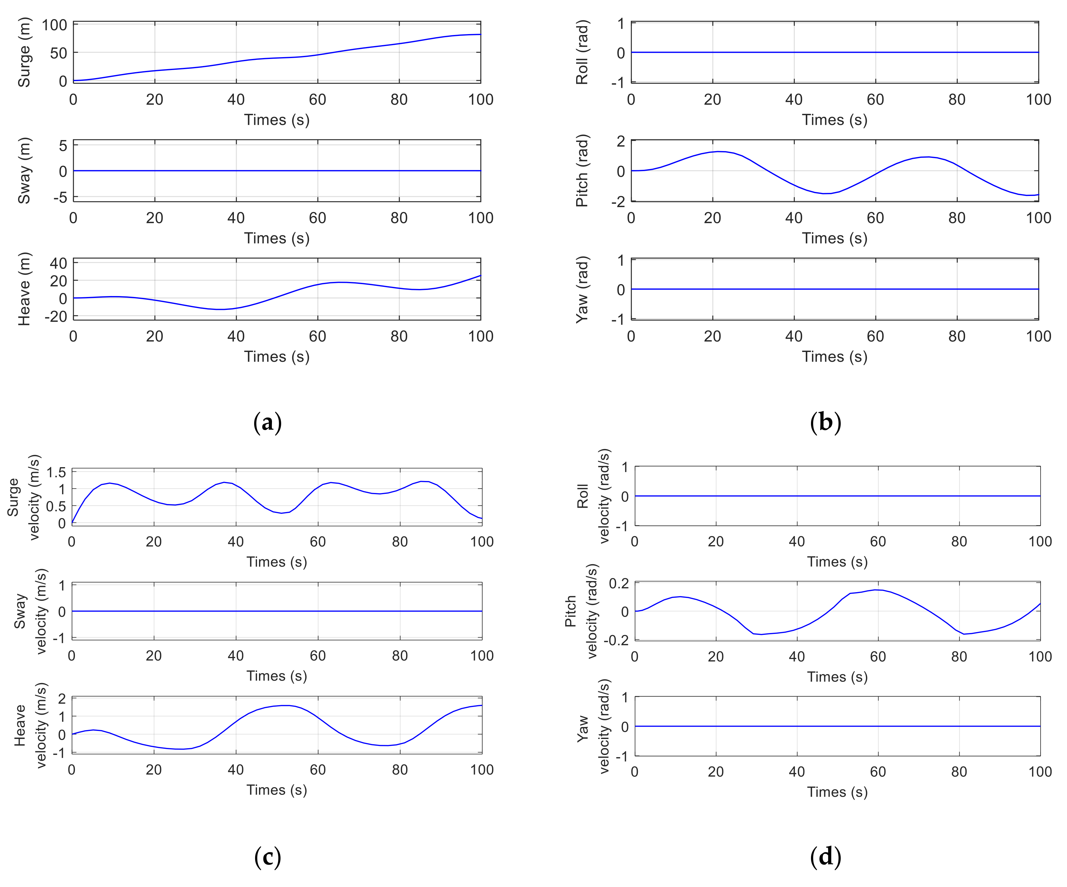
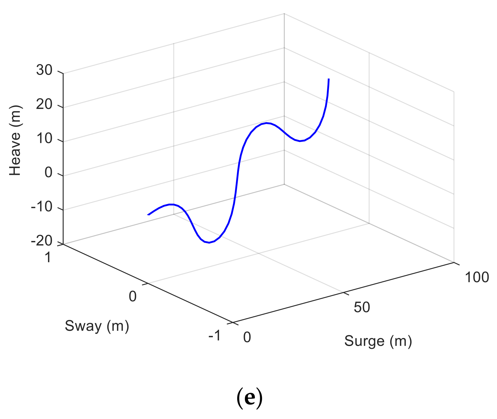
Figure 5 shows the simulation results of MJ-AUV’s pitching motion, and the pitching angle of joint 1 is set to ${\theta }_1=0^{\circ }$, the yaw angle of joint 1 is set to ${\psi }_1=0^{\circ }$, the pitch angle of joint 2 rotates in a sinusoidal manner with an amplitude of 20˚ and a period of 50 s, that ${\theta }_2={20}^{\circ }\sin (\frac{\pi t}{25})$, the yaw angle of joint 2 is set to ${\psi }_2=0^{\circ }$, and the thrust of the propeller is set to $T=60 \mathrm{N}$. The simulation duration is 100 s. It can be seen from Figure 5a,e that the vehicle has a tendency to move upwards, which is caused by the buoyancy force of the vehicle being greater than its gravity. During the pitching motion, the results in Figure 5a,c show that the vehicle has no change in displacement and velocity in the Y direction, while the results in Figure 5b,d show that the attitudes and angular velocities of the vehicle have no changes in the yaw and roll directions. Therefore, if the vehicle is only controlled in pitching motion, the relative state quantity of the three degrees of freedom can be zero, thus simplifying the complexity of the model.

Figure 6 shows the simulation results of the sinuous motion of the MJ-AUV. The pitching angle of joint 1 is set to ${\theta }_1=0^{\circ }$, the yaw angle of joint 1 rotates in a sinusoidal manner with an amplitude of 10˚ and a period of 50 s, i.e., ${\psi }_1={10}^{\circ }\sin (\frac{\pi t}{25})$, the pitch and yaw angle of joint 2 is set to 0˚, and the thrust of the propeller is set to $T=60 \mathrm{N}$. The simulation duration is 100 s. In the process of this movement, it can be seen from Figure 6b,d that the MJ-AUV is in roll motion. This is because when the yaw angle of the joint changes, the metacenter of the diversion cabin is not in the same vertical plane as the metacenter of the other cabins, so the roll moment is generated, and then the rolling phenomenon occurs.

Figure 7 shows the result of the spiral diving motion of the MJ-AUV. The pitching angle of joint 1 is set to ${\theta }_1=0^{\circ }$, the yaw angle of joint 1 is set to ${\psi }_1=5^{\circ }$, the pitch angle of joint 2 is set to ${\theta }_2={10}^{\circ }$, the pitch angle of joint 2 is set to, the yaw angle of joint 2 is set to ${\psi }_2=0^{\circ }$, and the thrust of the propeller is set to $T=60 \mathrm{N}$. The simulation duration is 1000 s. Unfortunately, it can be found from the results in Figure 7b,d that the rolling attitude of the vehicle is unstable, which is the same as that of the vehicle in the sinuous motion in Figure 7. It is all caused by the rolling moment that the metacenter of the diversion cabin is not in the same vertical plane as the metacenter of the other cabins. This brings a big problem for the multi-degree of freedom control.

The above simulation results are consistent with the common physical phenomena, and to a certain extent, it can be considered that the established MJ-AUV 3D dynamic model is reasonable, without loss of generality and reliability. According to the simulation results, compared with the single rigid body AUV, the MJ-AUV has stronger flexible maneuvering characteristics and can perform more complex movements, such as large angle pitching movement, small radius steering movement, spiral ascending and diving movement, and so on, which satisfies the design intention.

4.2. Model and Control Parameters

The initial states of the MJ-AUV are $\theta =0 \mathrm{rad}$, $\dot{\theta }=0 \mathrm{rad}$, ${\theta }_2=0 \mathrm{rad}$, $\psi =0 \mathrm{rad}$, $\dot{\psi }=0 \mathrm{rad}$, and ${\psi }_1=0 \mathrm{rad}$. In addition, the controller parameters are ${\omega }_0=30$, $b_{11}=0$, $b_{12}=0.1$, $b_{21}=0.1$, $b_{22}=0$, $Q=\mathrm{diag}\left(500,600,500,600\right)$, $R=\mathrm{diag}\left(0.1,0.1\right)$, and $\mathrm{diag}$ represents the diagonal matrix. The control gain after LQR optimization is

$$K=\left[\begin{array}{cccc}0& 0& -70.7107& 78.3672\\ -70.7107& 78.3672& 0& 0\end{array}\right].$$

4.3. Control Simulation

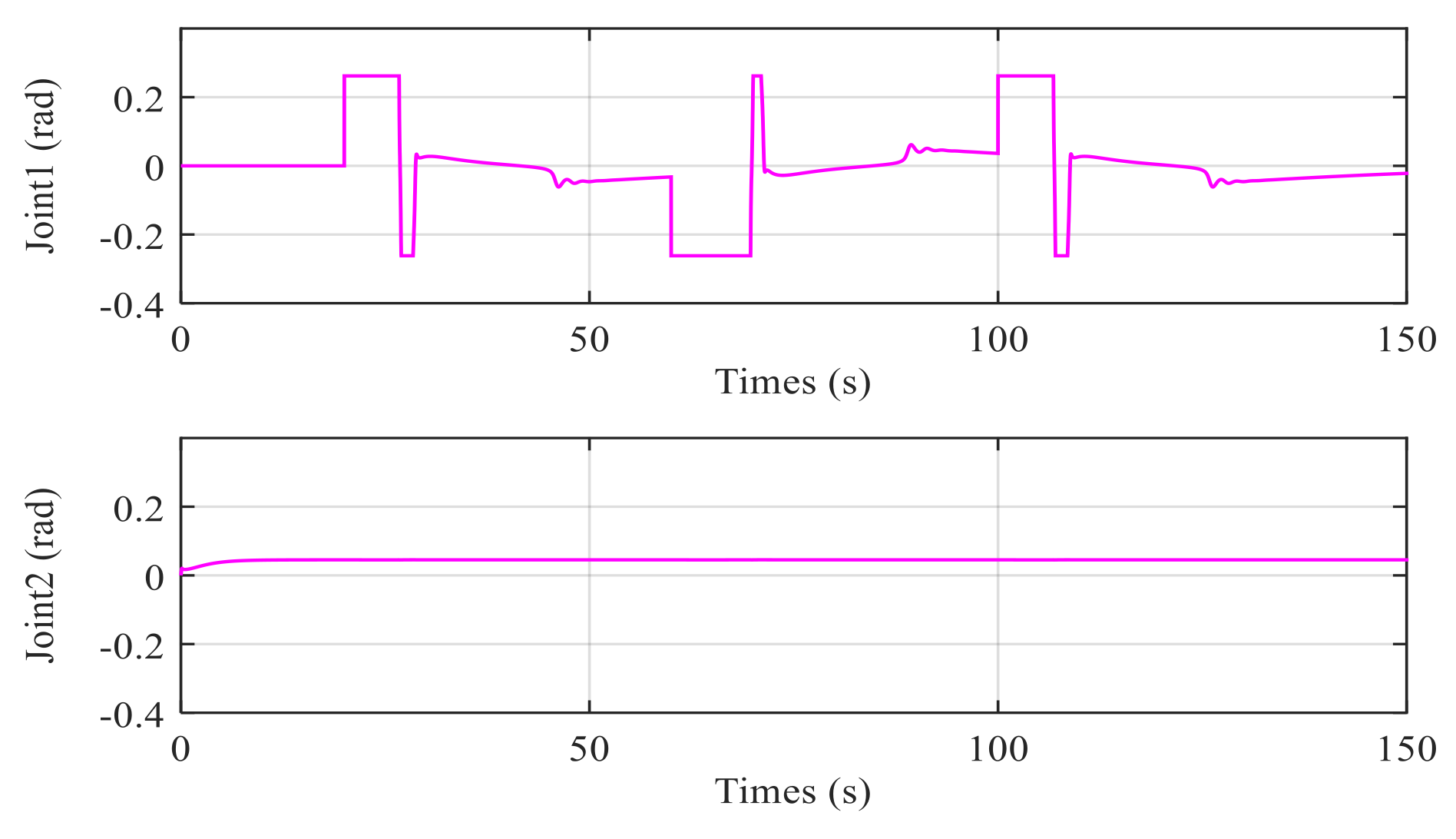
Figure 8, Figure 9, Figure 10, Figure 11 and Figure 12 show the simulation results of the pitch and yaw attitude control of the MJ-AUV, that is, when the pitch attitude is kept as 0 rad, the yaw attitude is adjusted according to the design signal. Figure 8 shows the pitch control results. The reason why the initial pitch attitude is not 0 rad is that the rest buoyancy of each cabin of MJ-AUV is positive, and the resultant moment of the body is not 0 rad. In other words, when the joint angle is 0 rad, the pitch attitude of the body is not 0 rad, so it is necessary to adjust the body attitude to 0 rad by adjusting the joint angle, which can also be seen from the performance of joint 2 in Figure 11. Figure 9 and the performance of joint 1 in Figure 11 show that, the yaw subsystem can be adjusted quickly after encountering multiple step signals, and the overshoot quantity is nearly 0 rad, with a very smooth transition process. Figure 10 shows that the maximum control error is within 0.005%, verifying that the designed controller has a high control accuracy. Figure 12 shows the observer’s estimation results for the total disturbance of the pitching and yaw subsystem. The results show that the estimated value of the total disturbance can follow the real value in real time and accurately, further proving the effectiveness of LESO and making a great contribution to the control of the disturbance compensation.

5. Conclusions

The main contributions of this paper are as follows:

(1)

A new type of MJ-AUV with orthogonal joints structure is proposed that can be used for the rapid exploration of the vertical profile of deep sea.

(2)

Considering the imbalance of gravity and buoyancy, a 3D analytical model of the MJ-AUV is established according to Newton’s second law and torque balance principle, which provides a theoretical basis for the study of the MJ-AUV’s 3D motion and model-based controller design.

(3)

The LQR decoupling control method based on LESO is proposed. The system is decoupled into pitch and yaw subsystems, and uses linear state observer to estimate and compensate for the total disturbance of each subsystem. LQR is used to achieve the optimal linear feedback control gain according to the expected input and output effects. It solves the problem of strong system coupling and makes the parameter tuning work more efficient.

(4)

The simulation results show that the improved control algorithm has the advantages of low overshot and high control precision, and the controller has the advantages of small computation, independence of the precise model of the system, and has a good prospect of engineering application.

References

- Zereik, E.; Bibuli, M.; Mišković, N.; Ridao, P.; Pascoal, A. Challenges and Future Trends in Marine Robotics. Annu. Rev. Control 2018, 46, 350–368. [Google Scholar] [CrossRef]
- Rudnick, D.L. Ocean Research Enabled by Underwater Gliders. Annu. Rev. Mar. Sci. 2016, 8, 519–541. [Google Scholar] [CrossRef] [PubMed]
- Yang, M.; Yang, S.; Wang, Y.; Liang, Y.; Wang, S.; Zhang, L. Optimization Design of Neutrally Buoyant Hull for Underwater Gliders. Ocean Eng. 2020, 209, 107512. [Google Scholar] [CrossRef]
- Wynn, R.B.; Huvenne, V.A.I.; Le Bas, T.P.; Murton, B.J.; Connelly, D.P.; Bett, B.J.; Ruhl, H.A.; Morris, K.J.; Peakall, J.; Parsons, D.R.; et al. Autonomous Underwater Vehicles (AUVs): Their Past, Present and Future Contributions to the Advancement of Marine Geoscience. Mar. Geol. 2014, 352, 451–468. [Google Scholar] [CrossRef] [Green Version]
- Xia, D. Dynamic Modeling of a Fishlike Robot with Undulatory Motion Based on Kane’s Method. J. Mech. Eng. 2009, 45, 41–49. [Google Scholar] [CrossRef]
- Tang, J.; Li, B.; Chang, J.; Wang, C. Design and Dynamic Model of Underwater Gliding Snake-like Robot. J. Huazhong Univ. Sci. Technol. Nat. Sci. 2018, 12, 89–94. [Google Scholar] [CrossRef]
- Kelasidi, E.; Liljeback, P.; Pettersen, K.Y.; Gravdahl, J.T. Innovation in Underwater Robots: Biologically Inspired Swimming Snake Robots. IEEE Robot. Autom. Mag. 2016, 23, 44–62. [Google Scholar] [CrossRef] [Green Version]
- Kelasidi, E.; Pettersen, K.Y.; Gravdahl, J.T.; Liljeback, P. Modeling of Underwater Snake Robots. In Proceedings of the 2014 IEEE International Conference on Robotics and Automation (ICRA), Hong Kong, China, 31 May–7 June 2014; pp. 4540–4547. [Google Scholar]
- Kelasidi, E.; Pettersen, K.Y.; Gravdahl, J.T. Modeling of Underwater Snake Robots Moving in a Vertical Plane in 3D. In Proceedings of the 2014 IEEE/RSJ International Conference on Intelligent Robots and Systems, Chicago, IL, USA, 14–18 September 2014; pp. 266–273. [Google Scholar]
- Koopaee, M.J.; Pretty, C.; Classens, K.; Chen, X. Dynamical Modeling and Control of Modular Snake Robots with Series Elastic Actuators for Pedal Wave Locomotion on Uneven Terrain. J. Mech. Des. 2020, 142. [Google Scholar] [CrossRef]
- Yu, J.; Liu, L.; Tan, M. Dynamic Modeling of Multi-Link Swimming Robot Capable of 3-D Motion. In Proceedings of the 2007 International Conference on Mechatronics and Automation, Harbin, China, 5–8 August 2007; pp. 1322–1327. [Google Scholar]
- Kohl, A.M.; Pettersen, K.Y.; Kelasidi, E.; Gravdahl, J.T. Planar Path Following of Underwater Snake Robots in the Presence of Ocean Currents. IEEE Robot. Autom. Lett. 2016, 1, 383–390. [Google Scholar] [CrossRef] [Green Version]
- Kelasidi, E.; Liljeback, P.; Pettersen, K.Y.; Gravdahl, J.T. Integral Line-of-Sight Guidance for Path Following Control of Underwater Snake Robots: Theory and Experiments. IEEE Trans. Robot. 2017, 33, 610–628. [Google Scholar] [CrossRef] [Green Version]
- Fischer, N.; Hughes, D.; Walters, P.; Schwartz, E.M.; Dixon, W.E. Nonlinear RISE-Based Control of an Autonomous Underwater Vehicle. IEEE Trans. Robot. 2014, 30, 845–852. [Google Scholar] [CrossRef] [Green Version]
- Zhao, S.; Yuh, J.; Choi, S.K. Adaptive DOB Control for AUVs. In Proceedings of the IEEE International Conference on Robotics and Automation (ICRA ’04), New Orleans, LA, USA, 26 April–1 May 2004; pp. 4899–4904. [Google Scholar]
- Wu, N.; Wu, C.; Ge, T.; Yang, D.; Yang, R. Pitch Channel Control of a REMUS AUV with Input Saturation and Coupling Disturbances. Appl. Sci. 2018, 8, 253. [Google Scholar] [CrossRef] [Green Version]
- Wang, T.; Wu, C.; Wang, J.; Ge, T. Modeling and Control of Negative-Buoyancy Tri-Tilt-Rotor Autonomous Underwater Vehicles Based on Immersion and Invariance Methodology. Appl. Sci. 2018, 8, 1150. [Google Scholar] [CrossRef] [Green Version]
- Kang, S.; Rong, Y.; Chou, W. Antidisturbance Control for AUV Trajectory Tracking Based on Fuzzy Adaptive Extended State Observer. Sensors 2020, 20, 7084. [Google Scholar] [CrossRef]
- Yangyang, Z.; Li’e, G.; Weidong, L.; Le, L. Research on Control Method of AUV Terminal Sliding Mode Variable Structure. In Proceedings of the 2017 International Conference on Robotics and Automation Sciences (ICRAS), Hong Kong, China, 26–29 August 2017; pp. 88–93. [Google Scholar]
- Rodriguez, J.; Castañeda, H.; Gordillo, J.L. Design of an Adaptive Sliding Mode Control for a Micro-AUV Subject to Water Currents and Parametric Uncertainties. JMSE 2019, 7, 445. [Google Scholar] [CrossRef] [Green Version]
- Huang, Z.; Liu, Y.; Zheng, H.; Wang, S.; Ma, J.; Liu, Y. A Self-Searching Optimal ADRC for the Pitch Angle Control of an Underwater Thermal Glider in the Vertical Plane Motion. Ocean Eng. 2018, 159, 98–111. [Google Scholar] [CrossRef]
- Zhang, Y.; Deng, H.; Li, Y. Depth Control of AUV Using Sliding Mode Active Disturbance Rejection Control. In Proceedings of the 2018 3rd International Conference on Advanced Robotics and Mechatronics (ICARM), Singapore, 18–20 July 2018; pp. 300–305. [Google Scholar]
- Shen, Y.; Shao, K.; Ren, W.; Liu, Y. Diving Control of Autonomous Underwater Vehicle Based on Improved Active Disturbance Rejection Control Approach. Neurocomputing 2016, 173, 1377–1385. [Google Scholar] [CrossRef]
- Wang, T.; Wang, J.; Wu, C.; Zhao, M.; Ge, T. Disturbance-Rejection Control for the Hover and Transition Modes of a Negative-Buoyancy Quad Tilt-Rotor Autonomous Underwater Vehicle. Appl. Sci. 2018, 8, 2459. [Google Scholar] [CrossRef] [Green Version]
- Li, H.; He, B.; Yin, Q.; Mu, X.; Zhang, J.; Wan, J.; Wang, D.; Shen, Y. Fuzzy Optimized MFAC Based on ADRC in AUV Heading Control. Electronics 2019, 8, 608. [Google Scholar] [CrossRef] [Green Version]
- Anderlini, E.; Parker, G.G.; Thomas, G. Docking Control of an Autonomous Underwater Vehicle Using Reinforcement Learning. Appl. Sci. 2019, 9, 3456. [Google Scholar] [CrossRef] [Green Version]
- Sun, Y.; Zhang, C.; Zhang, G.; Xu, H.; Ran, X. Three-Dimensional Path Tracking Control of Autonomous Underwater Vehicle Based on Deep Reinforcement Learning. JMSE 2019, 7, 443. [Google Scholar] [CrossRef] [Green Version]
- Sands, T. Development of Deterministic Artificial Intelligence for Unmanned Underwater Vehicles (UUV). JMSE 2020, 8, 578. [Google Scholar] [CrossRef]
- Gao, Z. Scaling and Bandwidth-Parameterization Based Controller Tuning. In Proceedings of the 2003 American Control Conference, Denver, CO, USA, 4–6 June 2003; Volume 6, pp. 4989–4996. [Google Scholar]
- Sudano, J.J. A Transformation of Unit Vectors to Simplify Derivations between Earth-Centered and Local North-East-and-up on an Ellipsoid Earth. In Proceedings of the IEEE 1995 National Aerospace and Electronics Conference (NAECON), Dayton, OH, USA, 22–26 May 1995; Volume 2, pp. 745–747. [Google Scholar]
- Gao, Z. Active Disturbance Rejection Control: A Paradigm Shift in Feedback Control System Design. In Proceedings of the 2006 American Control Conference, Minneapolis, MN, USA, 14–16 June 2006; pp. 2399–2405. [Google Scholar]
Figure 1.
Reference frames of the MJ-AUV.
Figure 2.
Orthogonal joint pitching motion.
Figure 3.
Orthogonal joint yaw motion.
Figure 4.
The structure of the LQR decoupling control method based on LESO.
Figure 5.
Pitching motion of MJ-AUV: (a) Position changes over time; (b) Attitude changes over time; (c) Linear velocity changes over time; (d) Angular velocity changes over time; (e) 3D motion.
Figure 6.
Yaw motion of the MJ-AUV: (a) Position changes over time; (b) Attitude changes over time; (c) Linear velocity changes over time; (d) Angular velocity changes over time; (e) 3D motion.
Figure 7.
Spiral dive motion of the MJ-AUV: (a) Position changes over time; (b) Attitude changes over time; (c) Linear velocity changes over time; (d) Angular velocity changes over time; (e) 3D motion.
Figure 8.
The pitching attitude of the MJ-AUV.
Figure 9.
The yaw attitude of the MJ-AUV.
Figure 10.
The feedback error of the MJ-AUV.
Figure 11.
The input of the MJ-AUV.
Figure 12.
The estimation of the total disturbances of the MJ-AUV.
Publisher’s Note: MDPI stays neutral with regard to jurisdictional claims in published maps and institutional affiliations. |
© 2021 by the authors. Licensee MDPI, Basel, Switzerland. This article is an open access article distributed under the terms and conditions of the Creative Commons Attribution (CC BY) license (http://creativecommons.org/licenses/by/4.0/).
Share and Cite
MDPI and ACS Style
Yu, L.; Meng, Q.; Zhang, H. 3-Dimensional Modeling and Attitude Control of Multi-Joint Autonomous Underwater Vehicles. J. Mar. Sci. Eng. 2021, 9, 307. https://0-doi-org.brum.beds.ac.uk/10.3390/jmse9030307
AMA Style
Yu L, Meng Q, Zhang H. 3-Dimensional Modeling and Attitude Control of Multi-Joint Autonomous Underwater Vehicles. Journal of Marine Science and Engineering. 2021; 9(3):307. https://0-doi-org.brum.beds.ac.uk/10.3390/jmse9030307
Chicago/Turabian StyleYu, Lin, Qinghao Meng, and Hongwei Zhang. 2021. "3-Dimensional Modeling and Attitude Control of Multi-Joint Autonomous Underwater Vehicles" Journal of Marine Science and Engineering 9, no. 3: 307. https://0-doi-org.brum.beds.ac.uk/10.3390/jmse9030307
Note that from the first issue of 2016, this journal uses article numbers instead of page numbers. See further details here.