
Dynamics and Distribution of Marine Synechococcus Abundance and Genotypes during Seasonal Hypoxia in a Coastal Marine Ranch

 , and
, and 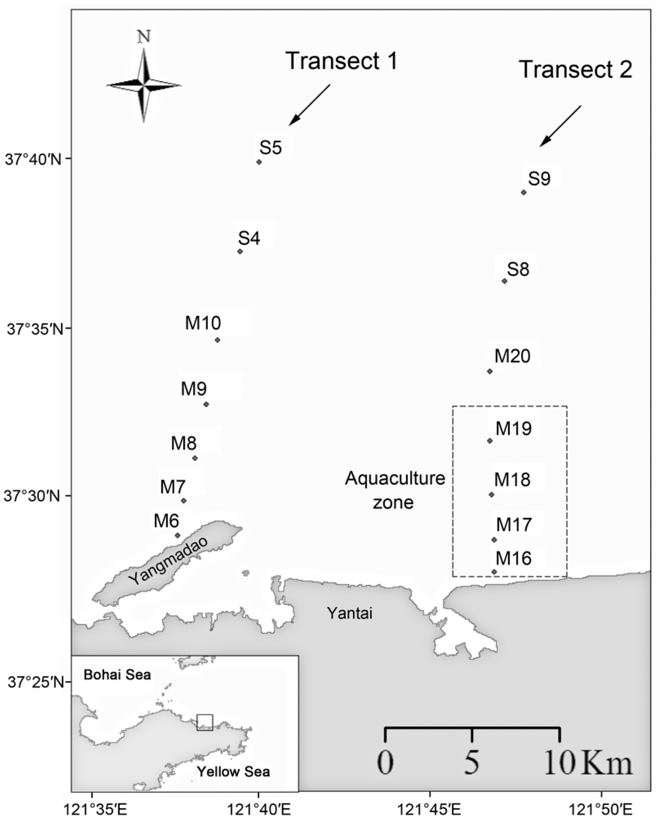
Abstract
:1. Introduction
2. Materials and Methods
2.1. Sampling and Environmental Data Collection
2.2. Flow Cytometry (FCM) Analysis
2.3. DNA Extraction and T-RFLP Analysis
2.4. Clone Library and Sequencing
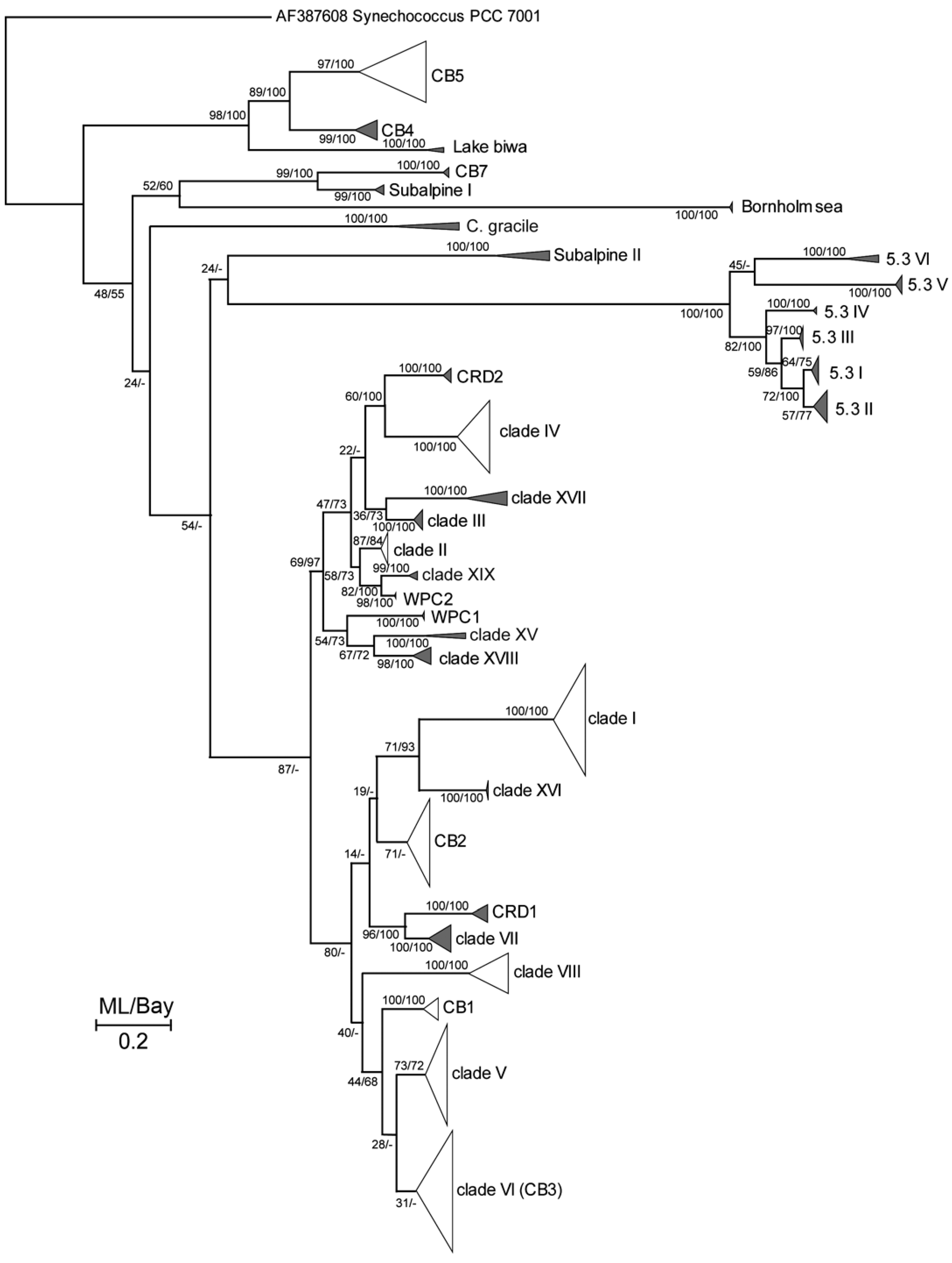
2.5. Phylogenetic Analysis
2.6. Statistical Analysis
3. Results
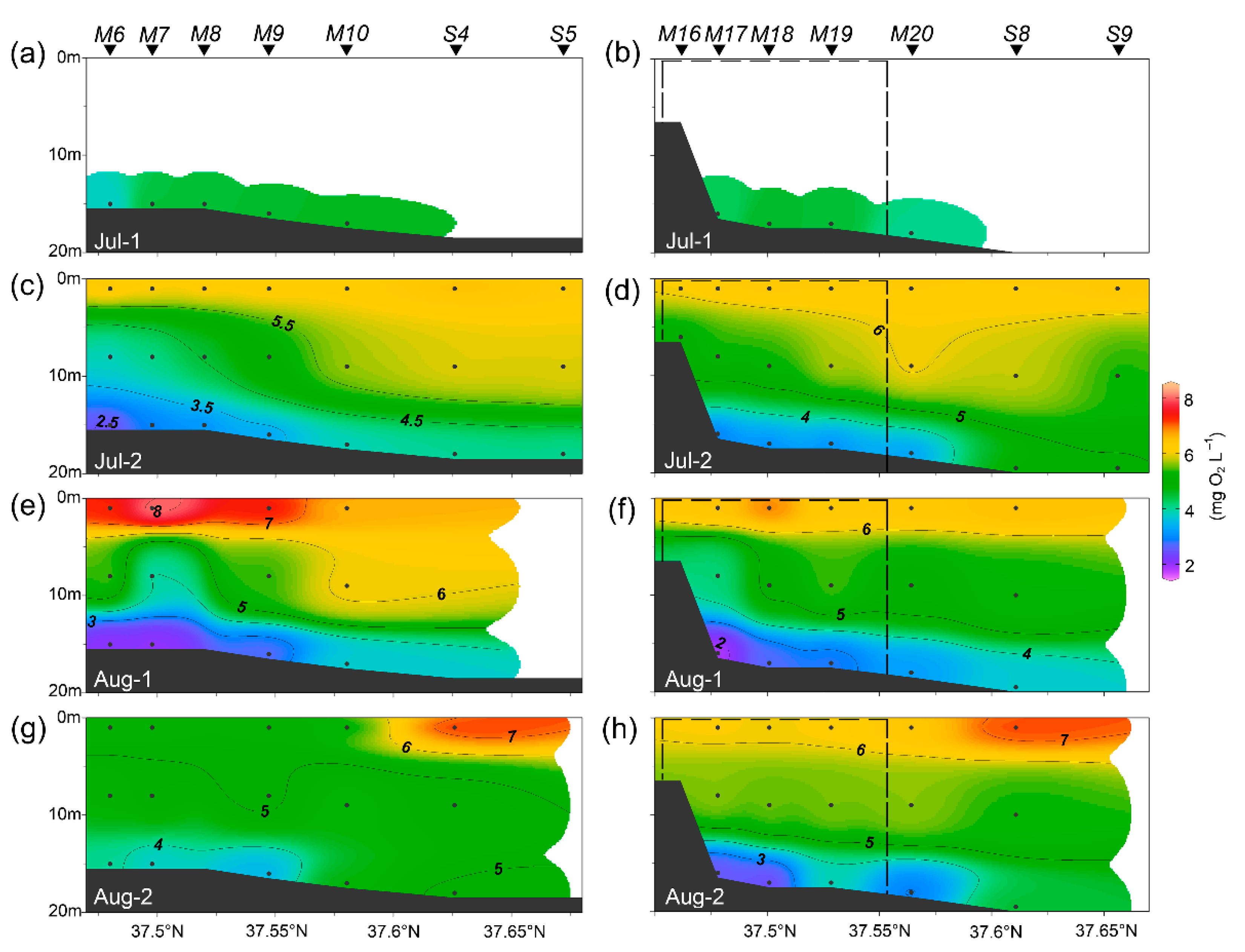
3.1. Environmental Conditions
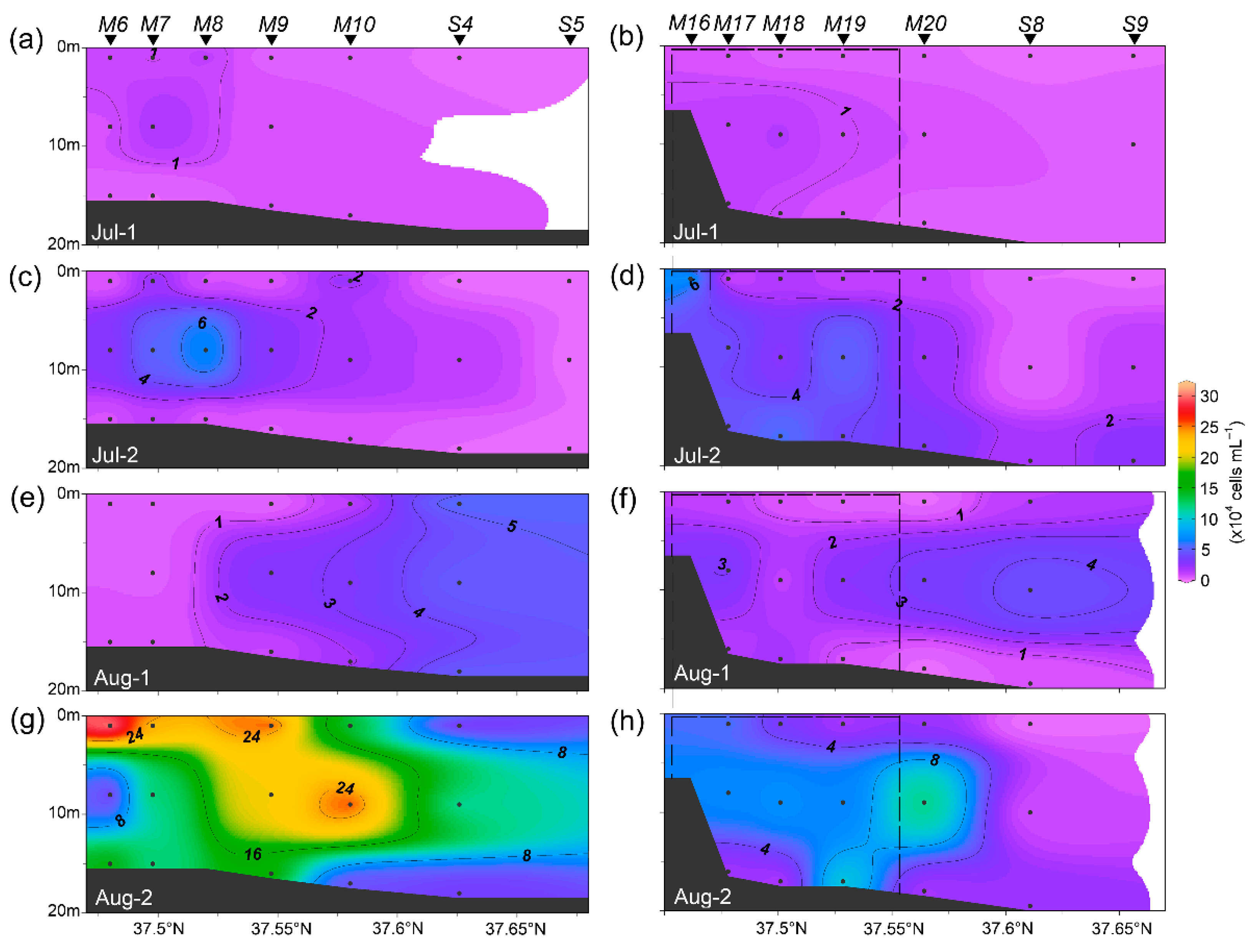
3.2. Cell Abundance of Synechococcus
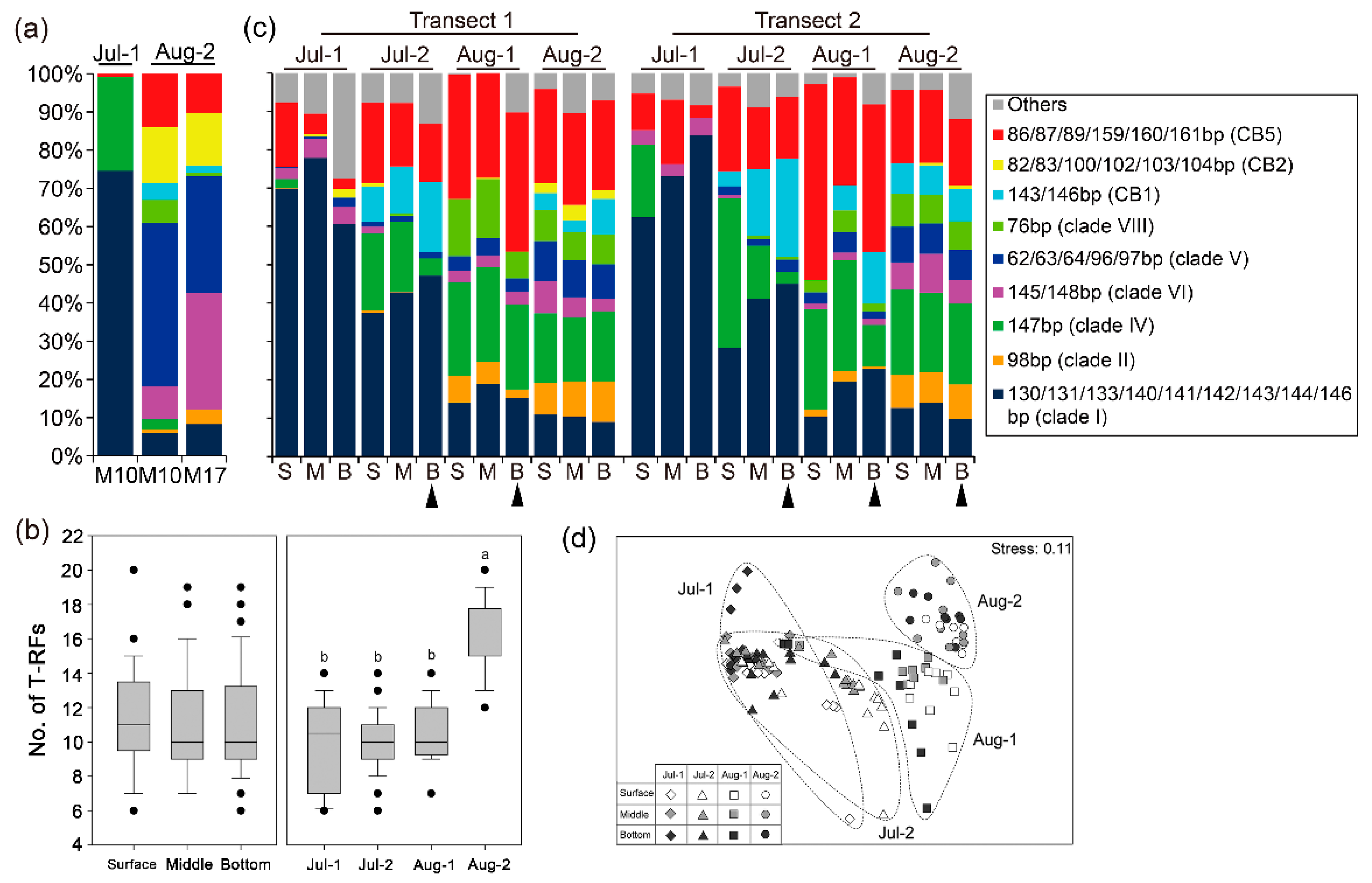
3.3. Richness and Composition of Synechococcus Genotypes
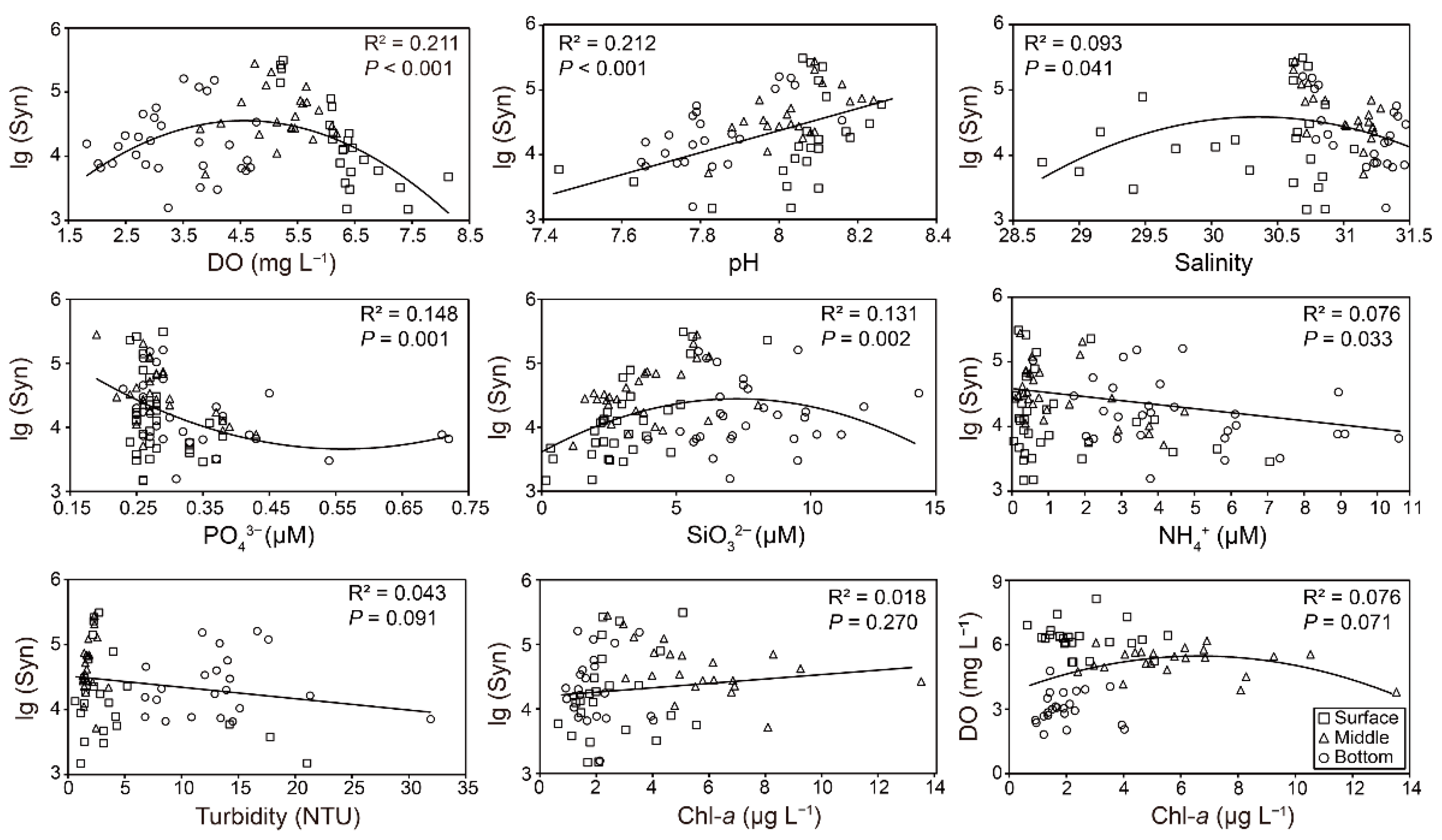
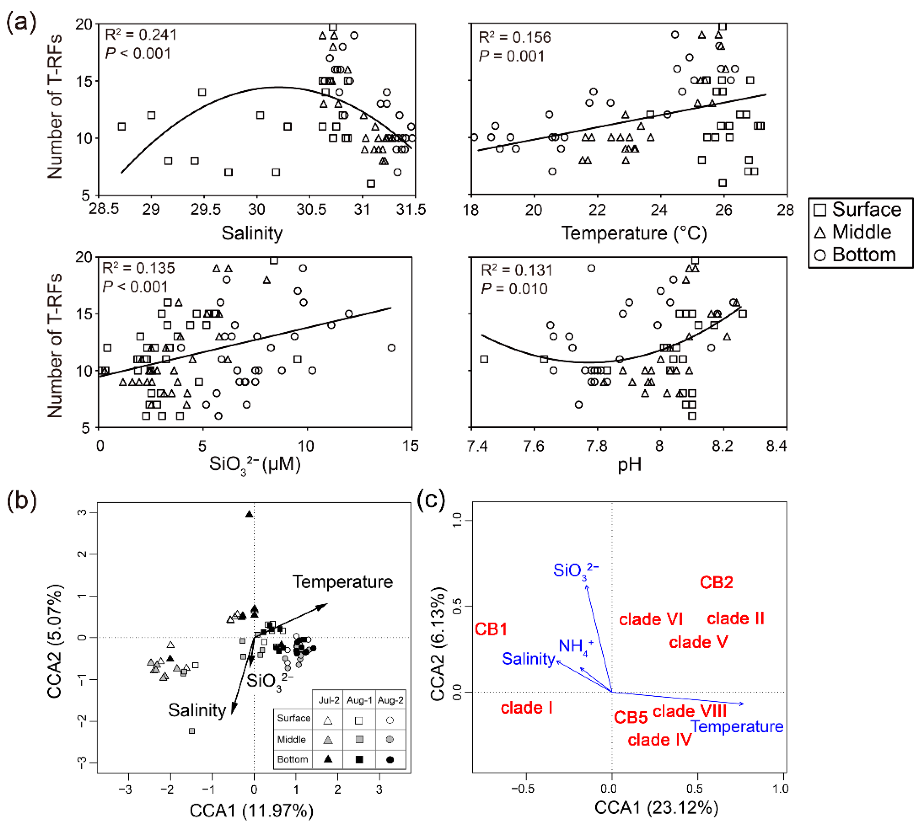
3.4. Relationships between Genotype Richness and Assemblage of Synechococcus and Environmental Factors
4. Discussion
Supplementary Materials
Author Contributions
Funding
Institutional Review Board Statement
Informed Consent Statement
Data Availability Statement
Conflicts of Interest
References
- Diaz, R.J.; Rosenberg, R. Spreading dead zones and consequences for marine ecosystems. Science 2008, 321, 926–929. [Google Scholar] [CrossRef] [PubMed]
- Howarth, R.; Chan, F.; Conley, D.J.; Garnier, J.; Doney, S.C.; Marino, R.; Billen, G. Coupled biogeochemical cycles: Eutrophication and hypoxia in temperate estuaries and coastal marine ecosystems. Front. Ecol. Environ. 2011, 9, 18–26. [Google Scholar] [CrossRef] [Green Version]
- Li, H.; Li, X.; Li, Q.; Liu, Y.; Song, J.; Zhang, Y. Environmental response to long-term mariculture activities in the Weihai coastal area, China. Sci. Total Environ. 2017, 601, 22–31. [Google Scholar] [CrossRef] [PubMed]
- Han, Q.; Wang, Y.; Zhang, Y.; Keesing, J.; Liu, D. Effects of intensive scallop mariculture on macrobenthic assemblages in Sishili Bay, the northern Yellow Sea of China. Hydrobiologia 2013, 718, 1–15. [Google Scholar] [CrossRef]
- Stramma, L.; Schmidtko, S.; Levin, L.A.; Johnson, G.C. Ocean oxygen minima expansions and their biological impacts. Deep Sea Res. 2010, 57 Pt I, 587–595. [Google Scholar] [CrossRef]
- Wright, J.J.; Konwar, K.M.; Hallam, S.J. Microbial ecology of expanding oxygen minimum zones. Nat. Rev. Microbiol. 2012, 10, 381–394. [Google Scholar] [CrossRef] [PubMed]
- Crump, B.C.; Peranteau, C.; Beckingham, B.; Cornwell, J.C. Respiratory succession and community succession of bacterioplankton in seasonally anoxic estuarine waters. Appl. Environ. Microbiol. 2007, 73, 6802–6810. [Google Scholar] [CrossRef] [Green Version]
- Parsons, R.J.; Nelson, C.E.; Carlson, C.A.; Denman, C.C.; Andersson, A.J.; Kledzik, A.L.; Vergin, K.L.; McNally, S.P.; Treusch, A.H.; Giovannoni, S.J. Marine bacterioplankton community turnover within seasonally hypoxic waters of a subtropical sound: Devil’s Hole, Bermuda. Environ. Microbiol. 2015, 17, 3481–3499. [Google Scholar] [CrossRef]
- Marañón, E.; Holligan, P.M.; Barciela, R.; González, N.; Mouriño, B.; Pazó, M.J.; Varela, M. Patterns of phytoplankton size structure and productivity in contrasting open-ocean environments. Mar. Ecol. Prog. Ser. 2001, 216, 43–56. [Google Scholar] [CrossRef] [Green Version]
- Waterbury, J.B.; Watson, S.W.; Guillard, R.R.; Brand, L.E. Widespread occurrence of a unicellular, marine, planktonic, cyanobacterium. Nature 1979, 277, 293–294. [Google Scholar] [CrossRef]
- Scanlan, D.J. Physiological diversity and niche adaptation in marine Synechococcus. Adv. Microb. Physiol. 2003, 47, 1–64. [Google Scholar] [PubMed]
- Partensky, F.; Blanchot, J.; Vaulot, D. Differential distribution and ecology of Prochlorococcus and Synechococcus in oceanic waters: A review. Bull. Inst. Oceanogr. Monaco 1999, 19, 457–476. [Google Scholar]
- Ahlgren, N.A.; Rocap, G. Culture isolation and culture-independent clone libraries reveal new marine Synechococcus ecotypes with distinctive light and N physiologies. Appl. Environ. Microbiol. 2006, 72, 7193–7204. [Google Scholar] [CrossRef] [PubMed] [Green Version]
- Lavin, P.; Gomez, P.; Gonzalez, B.; Ulloa, O. Diversity of the marine picocyanobacteria Prochlorococcus and Synechococcus assessed by terminal restriction fragment length polymorphisms of 16S-23S rRNA internal transcribed spacer sequences. Rev. Chil. Hist. Nat. 2008, 81, 515–531. [Google Scholar] [CrossRef]
- Lavin, P.; González, B.; Santibáñez, J.F.; Scanlan, D.J.; Ulloa, O. Novel lineages of Prochlorococcus thrive within the oxygen minimum zone of the eastern tropical South Pacific. Env. Microbiol. Rep. 2010, 2, 728–738. [Google Scholar] [CrossRef] [PubMed]
- Huang, S.; Wilhelm, S.W.; Harvey, H.R.; Taylor, K.; Jiao, N.; Chen, F. Novel lineages of Prochlorococcus and Synechococcus in the global oceans. ISME J. 2012, 6, 285–297. [Google Scholar] [CrossRef] [PubMed] [Green Version]
- Goericke, R.; Olson, R.J.; Shalapyonok, A. A novel niche for Prochlorococcus sp in low-light suboxic environments in the Arabian Sea and the Eastern Tropical North Pacific. Deep Sea Res. Part I 2000, 47, 1183–1205. [Google Scholar] [CrossRef]
- Pajares, S.; Varona-Cordero, F.; Hernández-Becerril, D.U. Spatial distribution patterns of bacterioplankton in the oxygen minimum zone of the tropical Mexican Pacific. Microb. Ecol. 2020, 80, 519–536. [Google Scholar] [CrossRef]
- Callieri, C.; Slabakova, V.; Dzhembekova, N.; Slabakova, N.; Peneva, E.; Cabello-Yeves, P.J.; Di Cesare, A.; Eckert, E.M.; Bertoni, R.; Corno, G. The mesopelagic anoxic Black Sea as an unexpected habitat for Synechococcus challenges our understanding of global “deep red fluorescence”. ISME J. 2019, 13, 1676–1687. [Google Scholar] [CrossRef] [PubMed] [Green Version]
- Yang, B.; Gao, X. Chromophoric dissolved organic matter in summer in a coastal mariculture region of northern Shandong Peninsula, North Yellow Sea. Cont. Shelf Res. 2019, 176, 19–35. [Google Scholar] [CrossRef]
- Yang, B.; Gao, X.; Xing, Q. Geochemistry of organic carbon in surface sediments of a summer hypoxic region in the coastal waters of northern Shandong Peninsula. Cont. Shelf Res. 2018, 171, 113–125. [Google Scholar] [CrossRef]
- Yang, B.; Gao, X.; Zhao, J.; Liu, Y.; Xie, L.; Lv, X.; Xing, Q. Potential linkage between sedimentary oxygen consumption and benthic flux of biogenic elements in a coastal scallop farming area, North Yellow Sea. Chemosphere 2021, 273, 129641. [Google Scholar] [CrossRef] [PubMed]
- Yang, B.; Gao, X.; Zhao, J.; Lu, Y.; Gao, T. Biogeochemistry of dissolved inorganic nutrients in an oligotrophic coastal mariculture region of the northern Shandong Peninsula, north Yellow Sea. Mar. Pollut. Bull. 2020, 150, 110693. [Google Scholar] [CrossRef]
- Gong, F.; Li, G.; Wang, Y.; Liu, Q.; Huang, F.; Yin, K.; Gong, J. Spatial shifts in size structure, phylogenetic diversity, community composition and abundance of small eukaryotic plankton in a coastal upwelling area of the northern South China Sea. J. Plankton Res. 2020, 42, 650–667. [Google Scholar] [CrossRef]
- Marie, D.; Partensky, F.; Jacquet, S.; Vaulot, D. Enumeration and cell cycle analysis of natural populations of marine picoplankton by flow cytometry using the nucleic acid stain SYBR Green I. Appl. Environ. Microbiol. 1997, 63, 186–193. [Google Scholar] [CrossRef] [Green Version]
- Fuchs, B.M.; Zubkov, M.V.; Sahm, K.; Burkill, P.H.; Amann, R. Changes in community composition during dilution cultures of marine bacterioplankton as assessed by flow cytometric and molecular biological techniques. Environ. Microbiol. 2000, 2, 191–201. [Google Scholar] [CrossRef] [PubMed]
- Cai, H.; Wang, K.; Huang, S.; Jiao, N.; Chen, F. Distinct patterns of picocyanobacterial communities in winter and summer in the Chesapeake Bay. Appl. Environ. Microbiol. 2010, 76, 2955–2960. [Google Scholar] [CrossRef] [Green Version]
- Huber, T.; Faulkner, G.; Hugenholtz, P. Bellerophon: A program to detect chimeric sequences in multiple sequence alignments. Bioinformatics 2004, 20, 2317–2319. [Google Scholar] [CrossRef]
- Katoh, K.; Misawa, K.; Kuma, K.I.; Miyata, T. MAFFT: A novel method for rapid multiple sequence alignment based on fast Fourier transform. Nucleic Acids Res. 2002, 30, 3059–3066. [Google Scholar] [CrossRef] [Green Version]
- Stamatakis, A. RAxML-VI-HPC: Maximum likelihood-based phylogenetic analyses with thousands of taxa and mixed models. Bioinformatics 2006, 22, 2688–2690. [Google Scholar] [CrossRef]
- Flombaum, P.; Gallegos, J.L.; Gordillo, R.A.; Rincón, J.; Zabala, L.L.; Jiao, N.; Karl, D.M.; Li, W.K.; Lomas, M.W.; Veneziano, D. Present and future global distributions of the marine cyanobacteria Prochlorococcus and Synechococcus. Proc. Natl. Acad. Sci. USA 2013, 110, 9824–9829. [Google Scholar] [CrossRef] [Green Version]
- Morel, A. Consequences of a Synechococcus bloom upon the optical properties of oceanic (case 1) waters. Limnol. Oceanogr. 1997, 42, 1746–1754. [Google Scholar] [CrossRef]
- Tai, V.; Palenik, B. Temporal variation of Synechococcus clades at a coastal Pacific Ocean monitoring site. ISME J. 2009, 3, 903–915. [Google Scholar] [CrossRef] [PubMed] [Green Version]
- Phlips, E.J.; Badylak, S.; Lynch, T.C. Blooms of the picoplanktonic cyanobacterium Synechococcus in Florida Bay, a subtropical inner-shelf lagoon. Limnol. Oceanogr. 1999, 44, 1166–1175. [Google Scholar] [CrossRef] [Green Version]
- Millette, N.; Kelble, C.; Linhoss, A.; Ashby, S.; Visser, L. Shift in baseline chlorophyll a concentration following a three-year Synechococcus bloom in southeastern Florida. Bull. Mar. Sci. 2018, 94, 3–19. [Google Scholar] [CrossRef]
- Li, J.; Chen, Z.; Jing, Z.; Zhou, L.; Li, G.; Ke, Z.; Jiang, X.; Liu, J.; Liu, H.; Tan, Y. Synechococcus bloom in the Pearl River Estuary and adjacent coastal area-With special focus on flooding during wet seasons. Sci. Total Environ. 2019, 692, 769–783. [Google Scholar] [CrossRef]
- Kilham, P.; Hecky, R.E. Comparative ecology of marine and freshwater phytoplankton. Limnol. Oceanogr. 1988, 33, 776–795. [Google Scholar] [CrossRef] [Green Version]
- Scanlan, D.J. Marine Picocyanobacteria. In Ecology of Cyanobacteria II: Their Diversity in Space and Time; Springer: Dordrecht, The Netherlands, 2012; pp. 503–533. [Google Scholar]
- Hutchins, D.A.; Witter, A.E.; Butler, A.; Luther, G.W. Competition among marine phytoplankton for different chelated iron species. Nature 1999, 400, 858–861. [Google Scholar] [CrossRef]
- Proctor, L.M.; Fuhrman, J.A. Viral mortality of marine bacteria and cyanobacteria. Nature 1990, 343, 60–62. [Google Scholar] [CrossRef]
- Tsai, A.Y.; Gong, G.C.; Huang, Y.W.; Chao, C.F. Estimates of bacterioplankton and Synechococcus spp. mortality from nanoflagellate grazing and viral lysis in the subtropical Danshui River estuary. Estuar. Coast. Shelf Sci. 2015, 153, 54–61. [Google Scholar] [CrossRef]
- Xia, X.; Vidyarathna, N.K.; Palenik, B.; Lee, P.; Liu, H. Comparison of the seasonal variations of Synechococcus assemblage structures in estuarine waters and coastal waters of Hong Kong. Appl. Environ. Microbiol. 2015, 81, 7644–7655. [Google Scholar] [CrossRef] [PubMed] [Green Version]
- Xia, X.; Cheung, S.; Endo, H.; Suzuki, K.; Liu, H. Latitudinal and vertical variation of Synechococcus assemblage composition along 170 degrees W transect from the South Pacific to the Arctic Ocean. Microb. Ecol. 2019, 77, 333–342. [Google Scholar] [CrossRef] [PubMed]
- Kim, Y.; Jeon, J.; Kwak, M.S.; Kim, G.H.; Koh, I.; Rho, M. Photosynthetic functions of Synechococcus in the ocean microbiomes of diverse salinity and seasons. PLoS ONE 2018, 13, e0190266. [Google Scholar] [CrossRef] [PubMed] [Green Version]
- Dufresne, A.; Ostrowski, M.; Scanlan, D.J.; Garczarek, L.; Mazard, S.; Palenik, B.P.; Paulsen, I.T.; de Marsac, N.T.; Wincker, P.; Dossat, C. Unraveling the genomic mosaic of a ubiquitous genus of marine cyanobacteria. Genome Biol. 2008, 9, R90. [Google Scholar] [CrossRef] [PubMed]
- Jing, H.; Liu, H.; Suzuki, K. Phylogenetic diversity of marine Synechococcus spp. in the Sea of Okhotsk. Aquat. Microb. Ecol. 2009, 56, 55–63. [Google Scholar] [CrossRef] [Green Version]
- Zwirglmaier, K.; Jardillier, L.; Ostrowski, M.; Mazard, S.; Garczarek, L.; Vaulot, D.; Not, F.; Massana, R.; Ulloa, O.; Scanlan, D.J. Global phylogeography of marine Synechococcus and Prochlorococcus reveals a distinct partitioning of lineages among oceanic biomes. Environ. Microbiol. 2008, 10, 147–161. [Google Scholar] [CrossRef] [PubMed]
- Zwirglmaier, K.; Heywood, J.L.; Chamberlain, K.; Woodward, E.M.S.; Zubkov, M.V.; Scanlan, D.J. Basin-scale distribution patterns lineages in the Atlantic Ocean. Environ. Microbiol. 2007, 9, 1278–1290. [Google Scholar] [CrossRef]
- Chen, F.; Wang, K.; Kan, J.; Suzuki, M.T.; Wommack, K.E. Diverse and unique picocyanobacteria in Chesapeake Bay, revealed by 16S-23S rRNA internal transcribed spacer sequences. Appl. Environ. Microbiol. 2006, 72, 2239–2243. [Google Scholar] [CrossRef] [Green Version]
- Choi, D.H.; Noh, J.H. Phylogenetic diversity of Synechococcus strains isolated from the East China Sea and the East Sea. FEMS Microbiol. Ecol. 2009, 69, 439–448. [Google Scholar] [CrossRef]
- Sohm, J.A.; Ahlgren, N.A.; Thomson, Z.J.; Williams, C.; Moffett, J.W.; Saito, M.A.; Webb, E.A.; Rocap, G. Co-occurring Synechococcus ecotypes occupy four major oceanic regimes defined by temperature, macronutrients and iron. ISME J. 2016, 10, 333–345. [Google Scholar] [CrossRef] [Green Version]
- Pittera, J.; Humily, F.; Thorel, M.; Grulois, D.; Garczarek, L.; Six, C. Connecting thermal physiology and latitudinal niche partitioning in marine Synechococcus. ISME J. 2014, 8, 1221–1236. [Google Scholar] [CrossRef] [PubMed]
- Sliwinska-Wilczewska, S.; Maculewicz, J.; Felpeto, A.B.; Vasconcelos, V.; Latala, A. Allelopathic activity of picocyanobacterium Synechococcus sp on filamentous cyanobacteria. J. Exp. Mar. Biol. Ecol. 2017, 496, 16–21. [Google Scholar] [CrossRef]
- Sliwinska-Wilczewska, S.; Felpeto, A.B.; Maculewicz, J.; Sobczyk, A.; Vasconcelos, V.; Latala, A. Allelopathic activity of the picocyanobacterium Synechococcus sp on unicellular eukaryote planktonic microalgae. Mar. Freshwater Res. 2018, 69, 1472–1479. [Google Scholar] [CrossRef]
- Bubak, I.; Śliwińska-Wilczewska, S.; Głowacka, P.; Szczerba, A.; Możdżeń, K. The importance of allelopathic picocyanobacterium Synechococcus sp. on the abundance, biomass formation, and structure of phytoplankton assemblages in three freshwater lakes. Toxins 2020, 12, 259. [Google Scholar] [CrossRef] [Green Version]


Publisher’s Note: MDPI stays neutral with regard to jurisdictional claims in published maps and institutional affiliations. |
© 2021 by the authors. Licensee MDPI, Basel, Switzerland. This article is an open access article distributed under the terms and conditions of the Creative Commons Attribution (CC BY) license (https://creativecommons.org/licenses/by/4.0/).
Share and Cite
Li, G.; Song, Q.; Zheng, P.; Zhang, X.; Zou, S.; Li, Y.; Gao, X.; Zhao, Z.; Gong, J. Dynamics and Distribution of Marine Synechococcus Abundance and Genotypes during Seasonal Hypoxia in a Coastal Marine Ranch. J. Mar. Sci. Eng. 2021, 9, 549. https://0-doi-org.brum.beds.ac.uk/10.3390/jmse9050549
Li G, Song Q, Zheng P, Zhang X, Zou S, Li Y, Gao X, Zhao Z, Gong J. Dynamics and Distribution of Marine Synechococcus Abundance and Genotypes during Seasonal Hypoxia in a Coastal Marine Ranch. Journal of Marine Science and Engineering. 2021; 9(5):549. https://0-doi-org.brum.beds.ac.uk/10.3390/jmse9050549
Chicago/Turabian StyleLi, Guihao, Qinqin Song, Pengfei Zheng, Xiaoli Zhang, Songbao Zou, Yanfang Li, Xuelu Gao, Zhao Zhao, and Jun Gong. 2021. "Dynamics and Distribution of Marine Synechococcus Abundance and Genotypes during Seasonal Hypoxia in a Coastal Marine Ranch" Journal of Marine Science and Engineering 9, no. 5: 549. https://0-doi-org.brum.beds.ac.uk/10.3390/jmse9050549