Multi-Attribute Group Decision-Making Based on Interval-Valued q-Rung Orthopair Fuzzy Power Generalized Maclaurin Symmetric Mean Operator and Its Application in Online Education Platform Performance Evaluation

Abstract

This paper aims to propose a novel multi-attribute group decision-making (MAGDM) method based on interval-valued q-rung orthopair fuzzy sets (IVq-ROFSs). The IVq-ROFSs have been proved to be effective in handling MAGDM problems, and several novel decision-making methods have been proposed. Nevertheless, it is worth pointing out that these approaches still have some limitations, and there still exist some realistic situations that cannot be solved by existing MAGDM methods. Hence, the objective of this paper is to introduce a novel MAGDM method, which can overcome some of the drawbacks of existing approaches. To effectively and appropriately aggregate interval-valued q-rung orthopair fuzzy numbers (IVq-ROFNs), we combine the power average with generalized Maclaurin symmetric mean (GMSM), propose the power GMSM operator and extend it into IVq-ROFSs. Afterwards, a collection of new aggregation operators for IVq-ROFNs are developed. In this paper, we study definitions of these operators and investigate their characteristics as well as special cases. Then, based on the new aggregation operators, we present a new MAGDM method. Finally, we apply the proposed MAGDM method in online education platform performance evaluation to illustrate its effectiveness and validity. In addition, we also provide comparative analysis to explain why decision-makers should use our method instead of the others.

1. Introduction

With the continuous development of information and communication technologies, the online education industry has ushered in new development opportunities, and many new online education platforms have emerged. Especially under the influence of the COVID-19 epidemic, many countries and regions have taken measures to close schools and switch to online teaching. Hence, online education platforms have obtained new development opportunities. In addition, the promotion of online education platforms can alleviate the unbalanced distribution of educational resources between regions, thereby promoting educational equity to a certain extent. Different online education platforms are quite different, and their quality and performance are also uneven. Therefore, it is necessary to evaluate the performance of online education platforms according to some methods.

The evaluation problem of online education platforms can be regarded as a multi-attribute group decision-making (MAGDM) problem essentially. Decision-makers evaluate different online education platforms from multiple dimensions, and on this basis, they can choose an appropriate method to determine the ranking order of online education platforms. Actually, MAGDM is a widely existing phenomenon, which has attracted increasing attention and interests in the fields of modern decision-making science, operational research, production and operation management, etc. There are many methodologies that help decision-makers to obtain the ranking results of possible alternatives. Recently, many scholars focused on MAGDM methods based on aggregation operators (AOs), which produce the final ranking orders of alternatives by integrating individual attribute values [1,2,3,4,5]. When using AOs to solve realistic MAGDM problems, to make the final decision results dependable and appropriate, we usually have to handle two kinds of situations. First, as different decision-makers have different background, priori knowledge and experience, they probably provide unbalanced evaluation values. In other words, in MAGDM process, some decision-makers may provide unduly high or low evaluation values, which, as a result, have significant negative impact on the final decision results. Second, attributes in realistic MAGDM problems are usually interrelated and such kinds of interrelationship among interactive attributes should be counted when calculating the overall evaluation values of alternatives.

For the first kind of decision-making situations, Yager [6] originated the power average (PA) operator, which is adequate to deal with decision-makers’ unreasonable or extreme evaluation values. It is worth pointing out that, however, the original PA operator was proposed for decision-making problems with crisp numbers. To make the PA operator more practical, many scholars focused on extending PA to complex decision-making environments. For example, Xu [7] and Wei and Lu [8] generalized PA into intuitionistic fuzzy sets and Pythagorean fuzzy sets, respectively. Wang et al. [9] introduced PA operators for dual hesitant fuzzy elements, and they applied the newly developed AOs into a safe path selection problem. Some other extensions and generalizations of PA into different fuzzy sets can be found in [10,11,12,13,14,15]. For the second kind of decision-making situations, some scholars started to study information AOs, which can consider the complex interrelationship among attributes. The Bonferroni mean (BM) [16] and Heronian mean (HM) [17] are two important AOs, which integrate not only the input arguments, but also the interrelationship among them. More and more scientists have realized the characteristics of BM and HM, and some novel fuzzy AOs have been proposed to deal with MAGDM problems. For BM, Xu and Yager [18], Yang et al. [19], Zhu and Xu [20], and Tu et al. [21] studied it under the circumstances of intuitionistic fuzzy sets, Pythagorean fuzzy sets, hesitant fuzzy sets, and dual hesitant fuzzy sets, respectively. Similar to BM, HM has also been a research hotspot and many new achievements have been reported in recent publications. For instance, Liu and Chen [22] first generalized HM into a fuzzy decision-making environment and introduced a collection of intuitionistic fuzzy HM operators. Liu and You [23] considered HM in linguistic intuitionistic fuzzy sets and proposed several novel AOs, which reflect the interrelationship among any two linguistic intuitionistic numbers. Yu et al. [24] presented dual hesitant fuzzy HM operators and applied them in a supplier selection problem. Similarly, Xu et al. [25] also investigated supplier selection problems under q-rung dual hesitant fuzzy sets based on HM. To date, HM is still a research hotspot and new MAGDM methods can still be found in newly published articles [26,27,28,29].

The above-mentioned references only focused on PA, BM or HM, respectively. As realistic decision-making issues are highly complicated, scholars also focused on hybrid AOs. In [30], authors proposed hesitant fuzzy power Bonferroni mean (PBM) operators and investigated their applications in hesitant fuzzy MAGDM problems. The main contributions and novelties are that they creatively combined PA with BM and put forward a hybrid AO, i.e., PBM. It is realized by scholars that PBM takes the merits of PA and BM, and it is more suitable to deal with practical MAGDM problems. After the introduction of PBM, Liu and Liu [31] studied it under linguistic intuitionistic fuzzy sets. Liu and Li [32] provided decision-makers an interval-valued intuitionistic fuzzy PBM operator based MAGDM method. Wang and Li [33] presented Pythagorean fuzzy interactive PBM operators and studied their applications in online payment service providers evaluation. Considering that HM has the similar function as BM, motivated by PBM, Liu [34] combined PA with HM and proposed power Heronian mean (PHM) operator and applied it in interval-valued intuitionistic fuzzy sets. Liu’s [34] contributions demonstrated the advantages and superiorities of PHM. Based on Liu’s [34] pioneering works, Ju et al. [35], Liu et al. [36], Wang et al. [37], Liu et al. [38], and Jiang et al. [39] investigated PHM under hesitant fuzzy linguistic sets, linguistic neutrosophic sets, q-rung orthopair hesitant fuzzy sets, neutrosophic cubic sets, and interval-valued dual hesitant fuzzy sets, respectively.

Recent publications reveal the advantages of PBM and PHM in aggregating fuzzy information, however, they still have drawbacks. One of the prominent drawbacks of PBM and PHM is that they only consider the interrelationship among any two attributes, which is insufficient and inadequate to handle some real MAGDM problems. More and more researches have indicated the importance and necessity of considering the interrelationship and interaction among multiple attributes [40]. Hence, it is necessary to combine PA with an AO, which considers the interrelationship among multiple arguments. The generalized Maclaurin symmetric mean (GMSM) [41] is an operator, which has the ability of reflecting the interrelationship among multiple input variables. In addition, GMSM has the ability of reflecting the individual importance of aggregated arguments, which makes it more powerful than the classical Maclaurin symmetric mean (MSM) [42]. Due to this reason, GMSM has been widely applied in Pythagorean fuzzy sets [43], q-rung orthopair fuzzy sets (q-ROFSs) [44], multi-hesitant fuzzy linguistic sets [45], intuitionistic fuzzy soft sets [46], probabilistic linguistic sets [47], etc. In this paper, considering the ability and flexibility of GMSM, we combine PA with GMSM and propose the power generalized Maclaurin symmetric mean (PGMSM) operator. Evidently, PGMSM is more powerful than PBM, PHM, and GMSM and is more suitable to deal with actual-life MAGDM problems. Additionally, we notice that the interval-valued q-ROFS (IVq-ROFS) proposed by Ju et al. [48] is a powerful information representation tool that can depict fuzziness and uncertainty efficiently. The IVq-ROFS is an extension of q-ROFS proposed by Yager [49]. MAGDM methods based on q-ROFSs have received much attention [50,51,52]. Similarly, some MAGDM methods under IVq-ROFSs have been proposed [53,54,55,56]. Nevertheless, these methods still have a drawback, i.e., they fail to handle the complicated interrelationship between attributes and simultaneously eliminate the bad influence of decision-makers’ evaluation values. In order to overcome this drawback, this paper extends PGMSM into IVq-ROFSs to propose a new MAGDM method.

The main contributions of this paper contain three aspects. First, a novel AO, called PGMSM is developed. Second, some new AOs for interval-valued q-rung orthopair fuzzy numbers (IVq-ROFNs) are developed. Finally, a new MAGDM method under IVq-ROFS circumstances is put forward. The rest of this paper is organized as follows. Section 2 recalls basic notions. Section 3 presents several new AOs for IVq-ROFNs and discusses their properties and characteristics. Based on the developed AOs, Section 4 presents a novel MAGDM method. Section 5 applies the proposed MAGDM method in online education performance evaluation. Section 6 summarizes the paper.

2. Basic Notions

This section introduces some basic notions that will be used in the following sections.

2.1. The Interval-Valued q-Rung Orthopair Fuzzy Sets

Definition 1

[48]. Let X be an ordinary fixed set, an IVq-ROFS A defined on X is expressed as

$$A=\left\{x,{\mu }_A\left(x\right),v_A\left(x\right)|x\in X\right\}$$

(1)

where ${\mu }_A\left(x\right),v_A\left(x\right)\subseteq \left[0,1\right]$ are two interval-valued values, denoting the membership and non-membership degrees of element $x\in X$ to the set A, such that ${\left(sup\left({\mu }_A\left(x\right)\right)\right)}^q+{\left(sup\left(v_A\left(x\right)\right)\right)}^q\le 1\left(q\ge 1\right)$. For convenience, the ordered pair $A=\left({\mu }_A\left(x\right),v_A\left(x\right)\right)$ is called an IVq-ROFN, which can be denoted as $\alpha =\left(\left[a,b\right],\left[c,d\right]\right)$ for simplicity, such that $a\le b$, $c\le d$, and $b^q+d^q\le 1\left(q\ge 1\right)$.

Basic operations of IVq-ROFNs are presented as follows:

Definition 2

[48]. Let $\alpha =\left(\left[a,b\right],\left[c,d\right]\right),$ ${\alpha }_1=\left(\left[a_1,b_1\right],\left[c_1,d_1\right]\right)$ and ${\alpha }_2=\left(\left[a_2,b_2\right],\left[c_2,d_2\right]\right)$ be any three IVq-ROFNs, and $\lambda$ be a positive real number, then

(1)

${\alpha }_1\oplus {\alpha }_2=\left(\left[{\left(a_1^q+a_2^q-a_1^q{a}_2^q\right)}^{1/q},{\left(b_1^q+b_2^q-b_1^q{b}_2^q\right)}^{1/q}\right],\left[c_1{c}_2,d_1{d}_2\right]\right)$;

(2)

${\alpha }_1\otimes {\alpha }_2=\left(\left[a_1{a}_2,b_1{b}_2\right],\left[{\left(c_1^q+c_2^q-c_1^q{c}_2^q\right)}^{1/q},{\left(d_1^q+d_2^q-d_1^q{d}_2^q\right)}^{1/q}\right]\right)$;

(3)

$\lambda \alpha =\left(\left[{\left(1-{\left(1-a^q\right)}^{\lambda }\right)}^{1/q},{\left(1-{\left(1-b^q\right)}^{\lambda }\right)}^{1/q}\right],\left[c^{\lambda },d^{\lambda }\right]\right)$;

(4)

${\alpha }^{\lambda }=\left(\left[a^{\lambda },b^{\lambda }\right],\left[{\left(1-{\left(1-c^q\right)}^{\lambda }\right)}^{1/q},{\left(1-{\left(1-d^q\right)}^{\lambda }\right)}^{1/q}\right]\right)$.

The method to compare any two IVq-ROFNs is presented as follows:

Definition 3

[48]. Let $\alpha =\left(\left[a,b\right],\left[c,d\right]\right)$ be an IVq-ROFN, then the score function of $\alpha$ is expressed as

$$S\left(\alpha \right)=\frac{2+a^q+b^q-c^q-d^q}{4}$$

(2)

and the accuracy function of $\alpha$ is expressed as

$$H\left(\alpha \right)=\frac{a^q+b^q+c^q+d^q}{2}$$

(3)

For any two IVq-ROFNs${\alpha }_1$and${\alpha }_2$

(1)

if$S\left({\alpha }_1\right)>S\left({\alpha }_2\right)$, then${\alpha }_1\ge {\alpha }_2$;

(2)

if$S\left({\alpha }_1\right)>S\left({\alpha }_2\right)$, then

• if$H\left({\alpha }_1\right)>H\left({\alpha }_2\right)$, then${\alpha }_1>{\alpha }_2$;
• if$H\left({\alpha }_1\right)=H\left({\alpha }_2\right)$, then${\alpha }_1={\alpha }_2$.

The distance measure between two IVq-ROFNs is defined as follows:

Definition 4.

Let${\alpha }_1=\left(\left[a_1,b_1\right],\left[c_1,d_1\right]\right)$and${\alpha }_2=\left(\left[a_2,b_2\right],\left[c_2,d_2\right]\right)$be two IVq-ROFNs, then the distance between${\alpha }_1$and${\alpha }_2$is defined as

$$d\left({\alpha }_1,{\alpha }_2\right)=\frac{\left|a_1^q-a_2^q\right|+\left|b_1^q-b_2^q\right|+\left|c_1^q-c_2^q\right|+\left|d_1^q-d_2^q\right|}{4}$$

(4)

2.2. The Power Average and Generalized Maclaurin Systems Mean Operators

Definition 5

[6]. Let $a_i\left(i=1,2,\dots ,n\right)$ be a collection of non-negative crisp numbers, then the PA operator is expressed as

$$PA\left(a_1,a_2,\dots ,a_n\right)=\frac{{\sum }_{i=1}^n\left(1+T\left(a_i\right)\right)a_i}{{\sum }_{i=1}^n\left(1+T\left(a_i\right)\right)}$$

(5)

where $T\left(a_i\right)={\sum }_{j=1,i\ne j}^{n}Sup\left(a_i,a_j\right)$, $Sup\left(a_i,a_j\right)$ denotes the support $a_i$ from $a_j$, satisfying the conditions

(1) 

$0\le Sup\left(a_i,a_j\right)\le 1$;

(2) 

$Sup\left(a_i,a_j\right)=Sup\left(a_j,a_i\right)$;

(3) 

$Sup\left(a,b\right)\le Sup\left(c,d\right)$, if$\left|a,b\right|\ge \left|c,d\right|$.

Definition 6

[41]. Let $a_i\left(i=1,2,\dots ,n\right)$ be a collection of crisp numbers, then the GMSM operator is defined as

$$GMS{M}^{\left(k,{\lambda }_1,{\lambda }_2,\dots ,{\lambda }_k\right)}\left(a_1,a_2,\dots ,a_n\right)={\left(\frac{{\sum }_{1\le i_1<\dots <i_k\le n}\left({\prod }_{j=1}^k{a}_{i_j}^{{\lambda }_j}\right)}{C_n^k}\right)}^{\frac{1}{{\lambda }_1+{\lambda }_2+\dots +{\lambda }_k}}$$

(6)

where ${\lambda }_1,{\lambda }_2,\dots ,{\lambda }_k\ge 0$, and $k=1,2,\dots ,n$ is an integer.

If we combine PA with GMSM, then the PGMSM operator is obtained.

Definition 7.

Let$a_i\left(i=1,2,\dots ,n\right)$be a collection of crisp numbers, then the PGMSM operator is defined as

$$\begin{array}{c}PGMS{M}^{\left(k,{\lambda }_1,{\lambda }_2,\dots ,{\lambda }_k\right)}\left(a_1,a_2,\dots ,a_n\right)\hfill \\ ={\left(\frac{{\sum }_{1\le i_1<\dots <i_k\le n}\left({\prod }_{j=1}^k{\left(\frac{n\left(1+T\left(a_{i_j}\right)\right)a_{i_j}}{{\sum }_{i=1}^n\left(1+T\left(a_i\right)\right)}\right)}^{{\lambda }_j}\right)}{C_n^k}\right)}^{\frac{1}{{\lambda }_1+{\lambda }_2+\dots +{\lambda }_k}}\hfill \end{array}$$

(7)

where${\lambda }_1,{\lambda }_2,\dots ,{\lambda }_k\ge 0$, and$k=1,2,\dots ,n$is an integer.$T\left(a_i\right)={\sum }_{j=1,i\ne j}^{n}Sup\left(a_i,a_j\right),$$Sup\left(a_i,a_j\right)$denotes the support for$a_i$from$a_j$, satisfying the properties presented in Definition 5. If${\gamma }_i=\left(1+T\left(a_i\right)\right)/{\sum }_{i=1}^n\left(1+T\left(a_i\right)\right)$, then Equation (7) can be written as

$$\begin{array}{c}PGMS{M}^{\left(k,{\lambda }_1,{\lambda }_2,\dots ,{\lambda }_k\right)}\left(a_1,a_2,\dots ,a_n\right)\hfill \\ ={\left(\frac{{\sum }_{1\le i_1<\dots <i_k\le n}\left({\prod }_{j=1}^k{\left(n{\gamma }_{i_j}{\alpha }_{i_j}\right)}^{{\lambda }_j}\right)}{C_n^k}\right)}^{\frac{1}{{\lambda }_1+{\lambda }_2+\dots +{\lambda }_k}}\hfill \end{array}$$

(8)

where$\gamma ={\left({\gamma }_1,{\gamma }_2,\dots ,{\gamma }_n\right)}^T$is called the power weight vector (PWV), such that$0\le {\gamma }_i\le 1$and${\sum }_{i=1}^n{\gamma }_i=1$.

In addition, we can obtain some special cases of the proposed PGMSM operator.

Case 1:

if$k=2$, then PGMSM operator is reduced to the PBM operator with the parameters${\lambda }_1$and${\lambda }_2$, i.e.,

$$\begin{array}{cc}\hfill PGMS{M}^{\left(2,{\lambda }_1,{\lambda }_2\right)}\left(a_1,a_2,\dots ,a_n\right)& ={\left(\frac{{\sum }_{1\le i_1<i_2\le n}\left({\left(n{\gamma }_{i_1}{a}_{i_1}\right)}^{{\lambda }_1}\times {\left(n{\gamma }_{i_2}{a}_{i_2}\right)}^{{\lambda }_2}\right)}{C_n^2}\right)}^{\frac{1}{{\lambda }_1+{\lambda }_2}}\hfill \\ & ={\left(\frac{2}{n\left(n-1\right)}{\sum }_{1\le i<j\le n}\left({\left(n{\gamma }_i{a}_i\right)}^{{\lambda }_1}\times {\left(n{\gamma }_j{a}_j\right)}^{{\lambda }_2}\right)\right)}^{\frac{1}{{\lambda }_1+{\lambda }_2}}\hfill \\ & ={\left(\frac{1}{n\left(n-1\right)}{\sum }_{1\le i,j\le n;i\ne j}\left({\left(n{\gamma }_i{a}_i\right)}^{{\lambda }_1}\times {\left(n{\gamma }_j{a}_j\right)}^{{\lambda }_2}\right)\right)}^{\frac{1}{{\lambda }_1+{\lambda }_2}}\hfill \\ & =PB{M}^{\left({\lambda }_1,{\lambda }_2\right)}\left(a_1,a_2,\dots ,a_n\right).\hfill \end{array}$$

(9)

Case 2:

if$k=3$, then PGMSM operator is reduced to the power generalized Bonferroni mean (PGBM) operator with the parameters${\lambda }_1$${\lambda }_2$and${\lambda }_3$, i.e.,

$$\begin{array}{c}PGMS{M}^{\left(3,{\lambda }_1,{\lambda }_2,{\lambda }_3\right)}\left(a_1,a_2,\dots ,a_n\right)\hfill \\ ={\left(\frac{{\sum }_{1\le i_1<i_2<i_3\le n}\left({\left(n{\gamma }_{i_1}{a}_{i_1}\right)}^{{\lambda }_1}\times {\left(n{\gamma }_{i_2}{a}_{i_2}\right)}^{{\lambda }_2}\times {\left(n{\gamma }_{i_3}{a}_{i_3}\right)}^{{\lambda }_3}\right)}{C_n^3}\right)}^{\frac{1}{{\lambda }_1+{\lambda }_2+{\lambda }_3}}\hfill \\ ={\left(\frac{6{\sum }_{1\le i_1<i_2<i_3\le n}\left({\left(n{\gamma }_{i_1}{a}_{i_1}\right)}^{{\lambda }_1}\times {\left(n{\gamma }_{i_2}{a}_{i_2}\right)}^{{\lambda }_2}\times {\left(n{\gamma }_{i_3}{a}_{i_3}\right)}^{{\lambda }_3}\right)}{n\left(n-1\right)\left(n-2\right)}\right)}^{\frac{1}{{\lambda }_1+{\lambda }_2+{\lambda }_3}}\hfill \\ ={\left(\frac{1}{n\left(n-1\right)\left(n-2\right)}{\displaystyle {\sum }_{i,j,l=1;i\ne j\ne l}^n}\left({\left(n{\gamma }_i{a}_i\right)}^{{\lambda }_1}\times {\left(n{\gamma }_j{a}_j\right)}^{{\lambda }_2}\times {\left(n{\gamma }_l{a}_l\right)}^{{\lambda }_3}\right)\right)}^{\frac{1}{{\lambda }_1+{\lambda }_2+{\lambda }_3}}\hfill \\ =PGB{M}^{\left(3,{\lambda }_1,{\lambda }_2,{\lambda }_3\right)}\left(a_1,a_2,\dots ,a_n\right)\hfill \end{array}$$

(10)

Case 3:

if${\lambda }_1={\lambda }_2=\dots ={\lambda }_k=1$, the PGMSM operator is reduced to the power Maclaurin symmetric mean (PMSM) operator, i.e.,

$$\begin{array}{cc}\hfill PGMS{M}^{\left(k,1,1,\dots ,1\right)}\left(a_1,a_2,\dots ,a_n\right)& ={\left(\frac{{\sum }_{1\le i_1<\dots <i_k\le n}\left({\prod }_{j=1}^{k}n{\gamma }_{i_j}{\alpha }_{i_j}\right)}{C_n^k}\right)}^{\frac{1}{k}}\hfill \\ & =PMS{M}^{\left(k\right)}\left(a_1,a_2,\dots ,a_n\right)\hfill \end{array}$$

(11)

3. Novel Aggregation Operators for IVq-ROFNs

In MAGDM problems, AOs are used to aggregate attribute values to determine comprehensive evaluation values of alternatives. Hence, based on the above-mentioned basic AOs, we introduce some novel AOs for IVq-ROFNs and discuss their properties.

3.1. The Interval-Valued q-Rung Orthopair Fuzzy Power Average Operator

We first extend the classical PA operator into IVq-ROFSs to propose a PA operator for IVq-ROFNs.

Definition 8.

Let${\alpha }_i=\left(\left[a_i,b_i\right],\left[c_i,d_i\right]\right)\left(i=1,2,\dots ,n\right)$be a collection of IVq-ROFNs, the interval-valued q-rung orthopair fuzzy power average (IVq-ROFPA) operator is defined as

$$IVqROFPA\left({\alpha }_1,{\alpha }_2,\dots ,{\alpha }_n\right)=\frac{{\oplus }_{i=1}^n\left(1+T\left(a_i\right)\right){\alpha }_i}{{\sum }_{i=1}^n\left(1+T\left(a_i\right)\right)},$$

(12)

where$T\left({\alpha }_i\right)={\sum }_{j=1,i\ne j}^{n}Sup\left({\alpha }_i,{\alpha }_j\right),$$Sup\left({\alpha }_i,{\alpha }_j\right)$denotes the support for${\alpha }_i$from${\alpha }_j$, satisfying the following conditions:

(1) 

$0\le Sup\left({\alpha }_i,{\alpha }_j\right)\le 1$;

(2) 

$Sup\left({\alpha }_i,{\alpha }_j\right)=Sup\left({\alpha }_j,{\alpha }_i\right)$;

(3) 

$Sup\left({\alpha }_i,{\alpha }_j\right)\le Sup\left({\alpha }_s,{\alpha }_t\right)$, if$dis\left({\alpha }_i,{\alpha }_j\right)\ge dis\left(\left({\alpha }_s,{\alpha }_t\right)\right)$.

If we assume

$${\varpi }_i=\frac{1+T\left({\alpha }_i\right)}{{\sum }_{i=1}^n\left(1+T\left({\alpha }_i\right)\right)},$$

(13)

then Equation (12) can be transformed into

$$IVqROFPA\left({\alpha }_1,{\alpha }_2,\dots ,{\alpha }_n\right)={\oplus }_{i=1}^n{\varpi }_i{\alpha }_i,$$

(14)

where$\varpi ={\left({\varpi }_1,{\varpi }_2,\cdots ,{\varpi }_n\right)}^T$is called the PWV, such that$0\le {\varpi }_i\le 1$and${\sum }_{i=1}^n{\varpi }_i=1$.

Based on the operational rules presented in Definition 2, the following aggregated results can be obtained.

Theorem 1.

Let${\alpha }_i=\left(\left[a_i,b_i\right],\left[c_i,d_i\right]\right)\left(i=1,2,\dots ,n\right)$be a collection of IVq-ROFNs, then the aggregated value by the IVq-ROFPA operator is still an IVq-ROFN and

$$\begin{array}{c}IVqROFPA\left({\alpha }_1,{\alpha }_2,\dots ,{\alpha }_n\right)\hfill \\ =\left(\left[{\left(1-{\prod }_{i=1}^n{\left(1-a_i^q\right)}^{{\varpi }_i}\right)}^{1/q},{\left(1-{\prod }_{i=1}^n{\left(1-b_i^q\right)}^{{\varpi }_i}\right)}^{1/q}\right],\left[{\prod }_{i=1}^n{c}_i^{{\varpi }_i},{\prod }_{i=1}^n{d}_i^{{\varpi }_i}\right]\right).\hfill \end{array}$$

(15)

Theorem 1 is trivial and we omit its proof. In addition, it is easy to prove that the IVq-ROFPA operator has the following properties.

Theorem 2

(Idempotency).Let${\alpha }_i\left(i=1,2,\dots ,n\right)$be a collection of IVq-ROFNs, if${\alpha }_i=\alpha =\left(\left[a,b\right],\left[c,d\right]\right)$for$i=1,2,\dots ,n$, then

$$IVqROFPA\left({\alpha }_1,{\alpha }_2,\dots ,{\alpha }_n\right)=\alpha$$

(16)

Theorem 3

(Boundedness).Let${\alpha }_i=\left(\left[a_i,b_i\right],\left[c_i,d_i\right]\right)\left(i=1,2,\dots ,n\right)$be a collection of IVq-ROFNs, then

$${\alpha }^{-}\le IVqROFPA\left({\alpha }_1,{\alpha }_2,\dots ,{\alpha }_n\right)\le {\alpha }^{+}$$

(17)

where

$${\alpha }^{+}=\left(\left[ma{x}_{i=1}^n{a}_i,ma{x}_{i=1}^n{b}_i\right],\left[mi{n}_{i=1}^n{c}_i,mi{n}_{i=1}^n{d}_i\right]\right),$$

and

$${\alpha }^{-}=\left(\left[mi{n}_{i=1}^n{a}_i,mi{n}_{i=1}^n{b}_i\right],\left[ma{x}_{i=1}^n{c}_i,ma{x}_{i=1}^n{d}_i\right]\right).$$

3.2. The Interval-Valued q-Rung Orthopair Fuzzy Power Weighted Average Operator

In MAGDM problem, when aggregating a collection of IVq-ROFNs, not only the IVq-ROFNs themselves, but also their corresponding weight information should be taken into account. Hence, we take into consideration of the weights of aggregated IVq-ROFNs in the IVq-ROFPA operator and propose its weighted form.

Definition 9.

Let${\alpha }_i=\left(\left[a_i,b_i\right],\left[c_i,d_i\right]\right)\left(i=1,2,\dots ,n\right)$be a collection of IVq-ROFNs and$w={\left(w_1,w_2,\dots ,w_n\right)}^T$be the corresponding weight vector, such that${\sum }_{i=1}^n{w}_i=1$ and $0\le w_i\le 1$. The interval-valued q-rung orthopair fuzzy power weighted average (IVq-ROFPWA) operator is defined as

$$IVqROFPWA\left({\alpha }_1,{\alpha }_2,\dots ,{\alpha }_n\right)=\frac{{\oplus }_{i=1}^n{w}_i\left(1+T\left(a_i\right)\right){\alpha }_i}{{\sum }_{i=1}^n{w}_i\left(1+T\left(a_i\right)\right)},$$

(18)

where $T\left({\alpha }_i\right)={\sum }_{j=1,i\ne j}^{n}Sup\left({\alpha }_i,{\alpha }_j\right),$ $Sup\left({\alpha }_i,{\alpha }_j\right)$ denotes the support for ${\alpha }_i$ from ${\alpha }_j$ , satisfying the properties presented in Definition 8. Similarly, we assume

$${\sigma }_i=\frac{w_i\left(1+T\left({\alpha }_i\right)\right)}{{\sum }_{i=1}^n{w}_i\left(1+T\left({\alpha }_i\right)\right)},$$

(19)

then, Equation (18) can be transformed into the following form

$$IVqROFPWA\left({\alpha }_1,{\alpha }_2,\dots ,{\alpha }_n\right)={\oplus }_{i=1}^n{\sigma }_i{\alpha }_i,$$

(20)

where $\sigma ={\left({\sigma }_1,{\sigma }_2,\dots {\sigma }_n\right)}^T$ is called the PWV, such that $0\le {\sigma }_i\le 1$ and ${\sum }_{i=1}^n{\sigma }_i=1$.

Simialrily, we can gain the following theorem.

Theorem 4.

Let${\alpha }_i=\left(\left[a_i,b_i\right],\left[c_i,d_i\right]\right)\left(i=1,2,\dots ,n\right)$be a collection of IVq-ROFNs, the aggregated value by the IVq-ROFPWA operator is still an IVq-ROFN and

$$\begin{array}{c}IVqROFPWA\left({\alpha }_1,{\alpha }_2,\dots ,{\alpha }_n\right)\hfill \\ =\left(\left[{\left(1-{\prod }_{i=1}^n\left(1-a_i^q\right)\right)}^{{\sigma }_i},{\left(1-{\prod }_{i=1}^n\left(1-b_i^q\right)\right)}^{{\sigma }_i}\right],\left[{\prod }_{i=1}^n{c}_i^{{\sigma }_i},{\prod }_{i=1}^n{d}_i^{{\sigma }_i}\right]\right).\hfill \end{array}$$

(21)

In addition, it is easy to prove that the IVq-ROFPWA operator has the properties of idempotency and boundedness.

3.3. The Interval-Valued q-Rung Orthopair Fuzzy Power Generalized Maclaurin Symmetric Mean Operator

In MAGDM problems, when fusing attribute values, we usually have to consider two significant issues, i.e., taking the interrelationship among attributes into consideration and reducing or eliminating the negative influence of decision-makers’ extreme evaluation values. The above-mentioned PGMSM takes the advantages of both PA and GMSM and, hence, it can resolve the above two issues. Therefore, in this subsection, we extend the PGMSM operator into IVq-ROFSs to propose a novel AO for IVq-ROFNs.

Definition 10.

Let${\alpha }_i=\left(\left[a_i,b_i\right],\left[c_i,d_i\right]\right)\left(i=1,2,\dots ,n\right)$be a collection of IVq-ROFNs, the interval-valued q-rung orthopair fuzzy power generalized Maclaurin symmetric mean (IVq-ROFPGMSM) operator is defined as

$$\begin{array}{c}IVqROFPGMS{M}^{\left(k,{\lambda }_1,{\lambda }_2,\dots ,{\lambda }_k\right)}\left({\alpha }_1,{\alpha }_2,\dots ,{\alpha }_n\right)\hfill \\ ={\left(\frac{{\oplus }_{1\le i_1<\dots <i_k\le n}\left({\otimes }_{j=1}^k{\left(\frac{n\left(1+T\left({\alpha }_i\right)\right)}{{\sum }_{i=1}^n\left(1+T\left({\alpha }_i\right)\right)}{\alpha }_{i_j}\right)}^{{\lambda }_j}\right)}{C_n^k}\right)}^{\frac{1}{{\lambda }_1+{\lambda }_2+\dots +{\lambda }_k}},\hfill \end{array}$$

(22)

where${\lambda }_1,{\lambda }_2,\dots ,{\lambda }_k\ge 0$, and$k=1,2,\dots ,n$is an integer.$T\left({\alpha }_i\right)={\sum }_{j=1,i\ne j}^{n}Sup\left({\alpha }_i,{\alpha }_j\right),$$Sup\left({\alpha }_i,{\alpha }_j\right)$denotes the support for${\alpha }_i$from${\alpha }_j$, satisfying the properties presented in Definition 8. Similarly, we assume

$${\eta }_i=\frac{1+T\left({\alpha }_i\right)}{{\sum }_{i=1}^n\left(1+T\left({\alpha }_i\right)\right)}$$

(23)

then Equation (22) can be transformed into

$$\begin{array}{c}IVqROFPGMS{M}^{\left(k,{\lambda }_1,{\lambda }_2,\dots ,{\lambda }_k\right)}\left({\alpha }_1,{\alpha }_2,\dots ,{\alpha }_n\right)\\ ={\left(\frac{{\oplus }_{1\le i_1<\dots <i_k\le n}\left({\otimes }_{j=1}^k{\left(n{\eta }_{i_j}{\alpha }_{i_j}\right)}^{{\lambda }_j}\right)}{C_n^k}\right)}^{\frac{1}{{\lambda }_1+{\lambda }_2+\dots +{\lambda }_k}},\hfill \end{array}$$

(24)

where$\eta ={\left({\eta }_1,{\eta }_2,\dots ,{\eta }_n\right)}^T$is called the PWV, such that$0\le {\eta }_i\le 1$and${\sum }_{i=1}^n{\eta }_i=1$.

Theorem 5.

Let${\alpha }_i=\left(\left[a_i,b_i\right],\left[c_i,d_i\right]\right)\left(i=1,2,\dots ,n\right)$be a collection of IVq-ROFNs, then the aggregated valued by the IVq-ROFPGMSM operator is also an IVq-ROFN and

$$\begin{array}{c}IVqROFPGMS{M}^{\left(k,{\lambda }_1,{\lambda }_2,\dots ,{\lambda }_k\right)}\left({\alpha }_1,{\alpha }_2,\dots ,{\alpha }_n\right)\hfill \\ =([{\left(1-{\prod }_{1\le i_1<\dots <i_k\le n}{\left(1-{\prod }_{j=1}^k{\left(1-{\left(1-a_{i_j}^q\right)}^{n{\eta }_{i_j}}\right)}^{{\lambda }_j}\right)}^{1/C_n^k}\right)}^{\frac{1}{q\left({\lambda }_1+{\lambda }_2+\dots +{\lambda }_k\right)}},\hfill \\ {\left(1-{\prod }_{1\le i_1<\dots <i_k\le n}{\left(1-{\prod }_{j=1}^k{\left(1-{\left(1-b_{i_j}^q\right)}^{n{\eta }_{i_j}}\right)}^{{\lambda }_j}\right)}^{1/C_n^k}\right)}^{\frac{1}{q\left({\lambda }_1+{\lambda }_2+\dots +{\lambda }_k\right)}}]\hfill \\ [{\left(1-{\left(1-{\prod }_{1\le i_1<\dots <i_k\le n}{\left(1-{\prod }_{j=1}^k{\left(1-c_{i_j}^{qn{\eta }_{i_j}}\right)}^{{\lambda }_j}\right)}^{1/C_n^k}\right)}^{\frac{1}{{\lambda }_1+{\lambda }_2+\dots +{\lambda }_k}}\right)}^{1/q}\hfill \\ {\left(1-{\left(1-{\prod }_{1\le i_1<\dots <i_k\le n}{\left(1-{\prod }_{j=1}^k{\left(1-c_{i_j}^{qn{\eta }_{i_j}}\right)}^{{\lambda }_j}\right)}^{1/C_n^k}\right)}^{\frac{1}{{\lambda }_1+{\lambda }_2+\dots +{\lambda }_k}}\right)}^{1/q}]).\hfill \end{array}$$

(25)

Proof. 

According to Definition 2, we have

$$n{\eta }_{i_j}{\alpha }_{i_j}=\left(\left[{\left(1-{\left(1-a_{i_j}^q\right)}^{n{\eta }_{i_j}}\right)}^{1/q},{\left(1-{\left(1-b_{i_j}^q\right)}^{n{\eta }_{i_j}}\right)}^{1/q}\right],\left[c_{i_j}^{n{\eta }_{i_j}},d_{i_j}^{n{\eta }_{i_j}}\right]\right),$$

and

$$\begin{array}{cc}\hfill {\left(n{\eta }_{i_j}{\alpha }_{i_j}\right)}^{{\lambda }_j}& =(\left[{\left(1-{\left(1-a_{i_j}^q\right)}^{n{\eta }_{i_j}}\right)}^{{\lambda }_j/q},{\left(1-{\left(1-b_{i_j}^q\right)}^{n{\eta }_{i_j}}\right)}^{{\lambda }_j/q}\right]\hfill \\ & \left[{\left(1-{\left(1-c_{i_j}^{qn{\eta }_{i_j}}\right)}^{{\lambda }_j}\right)}^{1/q},{\left(1-{\left(1-d_{i_j}^{qn{\eta }_{i_j}}\right)}^{{\lambda }_j}\right)}^{1/q}\right]).\hfill \end{array}$$

Hence,

$$\begin{array}{cc}\hfill {\otimes }_{j=1}^k{\left(n{\eta }_{i_j}{\alpha }_{i_j}\right)}^{{\lambda }_j}& =(\left[{\prod }_{j=1}^k{\left(1-{\left(1-a_{i_j}^q\right)}^{n{\eta }_{i_j}}\right)}^{{\lambda }_j/q},{\prod }_{j=1}^k{\left(1-{\left(1-b_{i_j}^q\right)}^{n{\eta }_{i_j}}\right)}^{{\lambda }_j/q}\right]\hfill \\ & \left[{\left(1-{\prod }_{j=1}^k{\left(1-c_{i_j}^{qn{\eta }_{i_j}}\right)}^{{\lambda }_j}\right)}^{1/q},{\left(1-{\prod }_{j=1}^k{\left(1-b_{i_j}^{qn{\eta }_{i_j}}\right)}^{{\lambda }_j}\right)}^{1/q}\right])\hfill \\ \hfill {\oplus }_{1\le i_1<\dots <i_k\le n}\left({\otimes }_{j=1}^k{\left(n{\eta }_{i_j}{\alpha }_{i_j}\right)}^{{\lambda }_j}\right)& =([{\left(1-{\prod }_{1\le i_1<\dots <i_k\le n}\left(1-{\prod }_{j=1}^k{\left(1-{\left(1-a_{i_j}^q\right)}^{n{\eta }_{i_j}}\right)}^{{\lambda }_j}\right)\right)}^{1/q},\hfill \\ & {\left(1-{\prod }_{1\le i_1<\dots <i_k\le n}\left(1-{\prod }_{j=1}^k{\left(1-{\left(1-a_{i_j}^q\right)}^{n{\eta }_{i_j}}\right)}^{{\lambda }_j}\right)\right)}^{1/q}]\hfill \\ & [{\prod }_{1\le i_1<\dots <i_k\le n}{\left(1-{\prod }_{j=1}^k{\left(1-c_{i_j}^{qn{\eta }_{i_j}}\right)}^{{\lambda }_j}\right)}^{1/q},\hfill \\ & {\prod }_{1\le i_1<\dots <i_k\le n}{\left(1-{\prod }_{j=1}^k{\left(1-d_{i_j}^{qn{\eta }_{i_j}}\right)}^{{\lambda }_j}\right)}^{1/q}])\hfill \end{array}$$

Further,

$$\begin{array}{c}\frac{{\oplus }_{1\le i_1<\dots <i_k\le n}\left({\otimes }_{j=1}^k{\left(n{\eta }_{i_j}{\alpha }_{i_j}\right)}^{{\lambda }_j}\right)}{C_n^k}\hfill \\ =([{\left(1-{\prod }_{1\le i_1<\dots <i_k\le n}{\left(1-{\prod }_{j=1}^k{\left(1-{\left(1-a_{i_j}^q\right)}^{n{\eta }_{i_j}}\right)}^{{\lambda }_j}\right)}^{1/C_n^k}\right)}^{1/q},\hfill \\ {\left(1-{\prod }_{1\le i_1<\dots <i_k\le n}{\left(1-{\prod }_{j=1}^k{\left(1-{\left(1-b_{i_j}^q\right)}^{n{\eta }_{i_j}}\right)}^{{\lambda }_j}\right)}^{1/C_n^k}\right)}^{1/q}])\hfill \\ [{\prod }_{1\le i_1<\dots <i_k\le n}{\left(1-{\prod }_{j=1}^k{\left(1-c_{i_j}^{qn{\eta }_{i_j}}\right)}^{{\lambda }_j}\right)}^{1/q{C}_n^k}\hfill \\ {\prod }_{1\le i_1<\dots <i_k\le n}{\left(1-{\prod }_{j=1}^k{\left(1-d_{i_j}^{qn{\eta }_{i_j}}\right)}^{{\lambda }_j}\right)}^{1/q{C}_n^k}]).\hfill \end{array}$$

Finally,

$$\begin{array}{c}{\left(\frac{{\oplus }_{1\le i_1<\dots <i_k\le n}\left({\otimes }_{j=1}^k{\left(n{\eta }_{i_j}{\alpha }_{i_j}\right)}^{{\lambda }_j}\right)}{C_n^k}\right)}^{\frac{1}{{\lambda }_1+{\lambda }_2+\dots +{\lambda }_k}}=\hfill \\ ([{\left(1-{\prod }_{1\le i_1<\dots <i_k\le n}{\left(1-{\prod }_{j=1}^k{\left(1-{\left(1-a_{i_j}^q\right)}^{n{\eta }_{i_j}}\right)}^{{\lambda }_j}\right)}^{1/C_n^k}\right)}^{\frac{1}{q\left({\lambda }_1+{\lambda }_2+\dots +{\lambda }_k\right)}},\hfill \\ {\left(1-{\prod }_{1\le i_1<\dots <i_k\le n}{\left(1-{\prod }_{j=1}^k{\left(1-{\left(1-b_{i_j}^q\right)}^{n{\eta }_{i_j}}\right)}^{{\lambda }_j}\right)}^{1/C_n^k}\right)}^{\frac{1}{q\left({\lambda }_1+{\lambda }_2+\dots +{\lambda }_k\right)}}]\hfill \\ [{\left(1-{\left(1-{\prod }_{1\le i_1<\dots <i_k\le n}{\left(1-{\prod }_{j=1}^k{\left(1-c_{i_j}^{qn{\eta }_{i_j}}\right)}^{{\lambda }_j}\right)}^{1/C_n^k}\right)}^{\frac{1}{{\lambda }_1+{\lambda }_2+\dots +{\lambda }_k}}\right)}^{1/q}\hfill \\ {\left(1-{\left(1-{\prod }_{1\le i_1<\dots <i_k\le n}{\left(1-{\prod }_{j=1}^k{\left(1-c_{i_j}^{qn{\eta }_{i_j}}\right)}^{{\lambda }_j}\right)}^{1/C_n^k}\right)}^{\frac{1}{{\lambda }_1+{\lambda }_2+\dots +{\lambda }_k}}\right)}^{1/q}]).\hfill \end{array}$$

It is worth investigating special cases of the proposed IVq-ROFPGMSM operator. First of all, we study special operators of IVq-ROFPGMSM operator with regarding of the parameter q.  □

Case 1:

if$q=1$, then IVq-ROFPGMSM becomes the interval-valued intuitionistic fuzzy PGMSM (IVIFPGMSM) operator, viz.,

$$\begin{array}{c}IVqROFPGMS{M}_{q=1}^{\left(k,{\lambda }_1,{\lambda }_2,\dots ,{\lambda }_k\right)}\left({\alpha }_1,{\alpha }_2,\dots ,{\alpha }_n\right)\hfill \\ =([{\left(1-{\prod }_{1\le i_1<\dots <i_k\le n}{\left(1-{\prod }_{j=1}^k{\left(1-{\left(1-a_{i_j}\right)}^{n{\eta }_{i_j}}\right)}^{{\lambda }_j}\right)}^{1/C_n^k}\right)}^{\frac{1}{{\lambda }_1+{\lambda }_2+\dots +{\lambda }_k}},\hfill \\ {\left(1-{\prod }_{1\le i_1<\dots <i_k\le n}{\left(1-{\prod }_{j=1}^k{\left(1-{\left(1-b_{i_j}\right)}^{n{\eta }_{i_j}}\right)}^{{\lambda }_j}\right)}^{1/C_n^k}\right)}^{\frac{1}{{\lambda }_1+{\lambda }_2+\dots +{\lambda }_k}}]\hfill \\ [{\left(1-{\left(1-{\prod }_{1\le i_1<\dots <i_k\le n}{\left(1-{\prod }_{j=1}^k{\left(1-c_{i_j}^{n{\eta }_{i_j}}\right)}^{{\lambda }_j}\right)}^{1/C_n^k}\right)}^{\frac{1}{{\lambda }_1+{\lambda }_2+\dots +{\lambda }_k}}\right)}^{1/q}\hfill \\ {\left(1-{\left(1-{\prod }_{1\le i_1<\dots <i_k\le n}{\left(1-{\prod }_{j=1}^k{\left(1-c_{i_j}^{n{\eta }_{i_j}}\right)}^{{\lambda }_j}\right)}^{1/C_n^k}\right)}^{\frac{1}{{\lambda }_1+{\lambda }_2+\dots +{\lambda }_k}}\right)}^{1/q}])\hfill \\ =IVIFPGMS{M}^{\left(k,{\lambda }_1,{\lambda }_2,\dots ,{\lambda }_k\right)}\left(k,{\lambda }_1,{\lambda }_2,\dots ,{\lambda }_k\right).\hfill \end{array}$$

(26)

Case 2:

if$q=2$, then IVq-ROFPGMSM becomes the interval-valued Pythagorean fuzzy PGMSM (IVPFPGMSM) operator, viz.,

$$\begin{array}{c}IVqROFPGMS{M}_{q=2}^{\left(k,{\lambda }_1,{\lambda }_2,\dots ,{\lambda }_k\right)}\left({\alpha }_1,{\alpha }_2,\dots ,{\alpha }_n\right)\hfill \\ =([{\left(1-{\prod }_{1\le i_1<\dots <i_k\le n}{\left(1-{\prod }_{j=1}^k{\left(1-{\left(1-a_{i_j}^2\right)}^{n{\eta }_{i_j}}\right)}^{{\lambda }_j}\right)}^{1/C_n^k}\right)}^{\frac{1}{2\left({\lambda }_1+{\lambda }_2+\dots +{\lambda }_k\right)}},\hfill \\ {\left(1-{\prod }_{1\le i_1<\dots <i_k\le n}{\left(1-{\prod }_{j=1}^k{\left(1-{\left(1-b_{i_j}^2\right)}^{n{\eta }_{i_j}}\right)}^{{\lambda }_j}\right)}^{1/C_n^k}\right)}^{\frac{1}{2\left({\lambda }_1+{\lambda }_2+\dots +{\lambda }_k\right)}}]\hfill \\ [{\left(1-{\left(1-{\displaystyle {\prod }_{1\le i_1<\dots <i_k\le n}}{\left(1-{\displaystyle {\prod }_{j=1}^k}{\left(1-c_{i_j}^{2n{\eta }_{i_j}}\right)}^{{\lambda }_j}\right)}^{1/C_n^k}\right)}^{\frac{1}{{\lambda }_1+{\lambda }_2+\dots +{\lambda }_k}}\right)}^{1/2}\hfill \\ {\left(1-{\left(1-{\prod }_{1\le i_1<\dots <i_k\le n}{\left(1-{\prod }_{j=1}^k{\left(1-c_{i_j}^{2n{\eta }_{i_j}}\right)}^{{\lambda }_j}\right)}^{1/C_n^k}\right)}^{\frac{1}{{\lambda }_1+{\lambda }_2+\dots +{\lambda }_k}}\right)}^{1/2}]).\hfill \\ =IVPFPGMS{M}^{\left(k,{\lambda }_1,{\lambda }_2,\dots ,{\lambda }_k\right)}\left({\alpha }_1,{\alpha }_2,\dots ,{\alpha }_n\right).\hfill \end{array}$$

(27)

Case 3:

if$q=3$, then IVq-ROFPGMSM becomes the interval-valued Fermatean fuzzy PGMSM (IVFFPGMSM) operator, viz.,

$$\begin{array}{c}IVqROFPGMS{M}_{q=3}^{\left(k,{\lambda }_1,{\lambda }_2,\dots ,{\lambda }_k\right)}\left({\alpha }_1,{\alpha }_2,\dots ,{\alpha }_n\right)\hfill \\ =([{\left(1-{\prod }_{1\le i_1<\dots <i_k\le n}{\left(1-{\prod }_{j=1}^k{\left(1-{\left(1-a_{i_j}^2\right)}^{n{\eta }_{i_j}}\right)}^{{\lambda }_j}\right)}^{1/C_n^k}\right)}^{\frac{1}{2\left({\lambda }_1+{\lambda }_2+\dots +{\lambda }_k\right)}},\hfill \\ {\left(1-{\prod }_{1\le i_1<\dots <i_k\le n}{\left(1-{\prod }_{j=1}^k{\left(1-{\left(1-b_{i_j}^2\right)}^{n{\eta }_{i_j}}\right)}^{{\lambda }_j}\right)}^{1/C_n^k}\right)}^{\frac{1}{2\left({\lambda }_1+{\lambda }_2+\dots +{\lambda }_k\right)}}]\hfill \\ [{\left(1-{\left(1-{\displaystyle {\prod }_{1\le i_1<\dots <i_k\le n}}{\left(1-{\displaystyle {\prod }_{j=1}^k}{\left(1-c_{i_j}^{2n{\eta }_{i_j}}\right)}^{{\lambda }_j}\right)}^{1/C_n^k}\right)}^{\frac{1}{{\lambda }_1+{\lambda }_2+\dots +{\lambda }_k}}\right)}^{1/2}\hfill \\ {\left(1-{\left(1-{\prod }_{1\le i_1<\dots <i_k\le n}{\left(1-{\prod }_{j=1}^k{\left(1-c_{i_j}^{2n{\eta }_{i_j}}\right)}^{{\lambda }_j}\right)}^{1/C_n^k}\right)}^{\frac{1}{{\lambda }_1+{\lambda }_2+\dots +{\lambda }_k}}\right)}^{1/2}]).\hfill \\ =IVFFPGMS{M}^{\left(k,{\lambda }_1,{\lambda }_2,\dots ,{\lambda }_k\right)}\left({\alpha }_1,{\alpha }_2,\dots ,{\alpha }_n\right).\hfill \end{array}$$

(28)

Additionally, we investigate some special cases of IVq-ROFPGMSM operator with regarding of the parameters in GMSM.

Case 4:

if$k=2$, then IVq-ROFPGMSM operator reduces to the interval-valued q-rung orthopair fuzzy power Bonferroni mean (IVq-ROFPBM) operator with the parameters${\lambda }_1$and${\lambda }_2$, viz.,

$$\begin{array}{c}IVqROFPGMS{M}^{\left(2,{\lambda }_1,{\lambda }_2\right)}\left({\alpha }_1,{\alpha }_2,\dots ,{\alpha }_n\right)={\left(\frac{1}{n\left(n-1\right)}{\oplus }_{i,j=1;i\ne j}^n\left({\left(n{\eta }_i{a}_i\right)}^{{\lambda }_1}\otimes {\left(n{\eta }_j{a}_j\right)}^{{\lambda }_2}\right)\right)}^{\frac{1}{{\lambda }_1+{\lambda }_2}}\hfill \\ ([{\left(1-{\left({\prod }_{i,j=1;i\ne j}^n\left(1-{\left(1-{\left(1-a_i^q\right)}^{n{\eta }_i}\right)}^{{\lambda }_1}\times {\left(1-{\left(1-a_j^q\right)}^{n{\eta }_j}\right)}^{{\lambda }_2}\right)\right)}^{\frac{1}{n\left(n-1\right)}}\right)}^{\frac{1}{q\left({\lambda }_1+{\lambda }_2\right)}},\hfill \\ {\left(1-{\left({\prod }_{i,j=1;i\ne j}^n\left(1-{\left(1-{\left(1-b_i^q\right)}^{n{\eta }_i}\right)}^{{\lambda }_1}\times {\left(1-{\left(1-b_j^q\right)}^{n{\eta }_j}\right)}^{{\lambda }_2}\right)\right)}^{\frac{1}{n\left(n-1\right)}}\right)}^{\frac{1}{q\left({\lambda }_1+{\lambda }_2\right)}}],\hfill \\ [{\left(1-{\left(1-{\prod }_{i,j=1;i\ne j}^n{\left(1-{\left(1-c_i^{qn{\eta }_i}\right)}^{{\lambda }_1}\times {\left(1-c_j^{qn{\eta }_j}\right)}^{{\lambda }_2}\right)}^{\frac{1}{n\left(n-1\right)}}\right)}^{\frac{1}{{\lambda }_1+{\lambda }_2}}\right)}^{1/q},\hfill \\ {\left(1-{\left(1-{\prod }_{i,j=1;i\ne j}^n{\left(1-{\left(1-d_i^{qn{\eta }_i}\right)}^{{\lambda }_1}\times {\left(1-d_j^{qn{\eta }_j}\right)}^{{\lambda }_2}\right)}^{\frac{1}{n\left(n-1\right)}}\right)}^{\frac{1}{{\lambda }_1+{\lambda }_2}}\right)}^{1/q}])\hfill \\ =IVqROFPB{M}^{\left({\lambda }_1,{\lambda }_2\right)}\left({\alpha }_1,{\alpha }_2,\dots ,{\alpha }_n\right),\hfill \end{array}$$

(29)

Additionally, if the value $Sup\left({\alpha }_i,{\alpha }_j\right)$ is a non-negative number, then IVq-ROFPGMSM operator further reduces to the interval-valued q-rung orthopair fuzzy Bonferroni mean (IVq-ROFBM) operator, i.e.,

$$\begin{array}{c}IVqROFPGMS{M}^{\left(2,{\lambda }_1,{\lambda }_2\right)}\left({\alpha }_1,{\alpha }_2,\dots ,{\alpha }_n\right)={\left(\frac{1}{n\left(n-1\right)}{\oplus }_{i,j=1;i\ne j}^n\left(a_i^{{\lambda }_1}\otimes a_j^{{\lambda }_2}\right)\right)}^{\frac{1}{{\lambda }_1+{\lambda }_2}}\hfill \\ (\left[{\left(1-{\left({\prod }_{i,j=1}^n\left(1-{\left(a_i^{{\lambda }_1}{a}_j^{{\lambda }_2}\right)}^q\right)\right)}^{\frac{1}{n\left(n-1\right)}}\right)}^{\frac{1}{q\left({\lambda }_1+{\lambda }_2\right)}},{\left(1-{\left({\prod }_{i,j=1}^n\left(1-{\left(b_i^{{\lambda }_1}{b}_j^{{\lambda }_2}\right)}^q\right)\right)}^{\frac{1}{n\left(n-1\right)}}\right)}^{\frac{1}{q\left({\lambda }_1+{\lambda }_2\right)}}\right],\hfill \\ [{\left(1-{\left(1-{\prod }_{i,j=1}^n{\left(1-{\left(1-c_i^q\right)}^{{\lambda }_1}\times {\left(1-c_j^q\right)}^{{\lambda }_2}\right)}^{\frac{1}{n\left(n-1\right)}}\right)}^{\frac{1}{{\lambda }_1+{\lambda }_2}}\right)}^{1/q},\hfill \\ {\left(1-{\left(1-{\prod }_{i,j=1}^n{\left(1-{\left(1-d_i^q\right)}^{{\lambda }_1}\times {\left(1-d_j^q\right)}^{{\lambda }_2}\right)}^{\frac{1}{n\left(n-1\right)}}\right)}^{\frac{1}{{\lambda }_1+{\lambda }_2}}\right)}^{1/q}])\hfill \\ =IVqROFB{M}^{\left({\lambda }_1,{\lambda }_2\right)}\left({\alpha }_1,{\alpha }_2,\dots ,{\alpha }_n\right).\hfill \end{array}$$

(30)

Case 5:

if$k=3$, the IVq-ROFPGMSM operator reduces to the interval-valued q-rung orthopair fuzzy power generalized Bonferroni mean (IVq-ROFPGBM) operator with the parameters${\lambda }_1,$${\lambda }_2$and${\lambda }_3$, viz.

$$\begin{array}{c}IVqROFPGMS{M}^{\left(3,{\lambda }_1,{\lambda }_2,{\lambda }_3\right)}\left({\alpha }_1,{\alpha }_2,\dots ,{\alpha }_n\right)\hfill \\ ={\left(\frac{1}{n\left(n-1\right)\left(n-2\right)}{\oplus }_{i,j,l=1;i\ne j\ne l}^n\left({\left(n{\eta }_i{a}_i\right)}^{{\lambda }_1}\otimes {\left(n{\eta }_j{a}_j\right)}^{{\lambda }_2}\otimes {\left(n{\eta }_l{a}_l\right)}^{{\lambda }_3}\right)\right)}^{\frac{1}{{\lambda }_1+{\lambda }_2+{\lambda }_3}}\hfill \\ =([{\left(1-{\prod }_{i,j,l=1;i\ne j\ne l}^n{\left(1-{\left(1-{\left(1-a_i^q\right)}^{n{\eta }_i}\right)}^{{\lambda }_1}\times {\left(1-{\left(1-a_j^q\right)}^{n{\eta }_j}\right)}^{{\lambda }_2}\times {\left(1-{\left(1-a_l^q\right)}^{n{\eta }_l}\right)}^{{\lambda }_3}\right)}^{\frac{1}{n\left(n-1\right)\left(n-2\right)}}\right)}^{\frac{1}{q\left({\lambda }_1+{\lambda }_2+{\lambda }_3\right)}},\hfill \\ {\left(1-{\prod }_{i,j,l=1;i\ne j\ne l}^n{\left(1-{\left(1-{\left(1-b_i^q\right)}^{n{\eta }_i}\right)}^{{\lambda }_1}\times {\left(1-{\left(1-b_j^q\right)}^{n{\eta }_j}\right)}^{{\lambda }_2}\times {\left(1-{\left(1-b_l^q\right)}^{n{\eta }_l}\right)}^{{\lambda }_3}\right)}^{\frac{1}{n\left(n-1\right)\left(n-2\right)}}\right)}^{\frac{1}{q\left({\lambda }_1+{\lambda }_2+{\lambda }_3\right)}}],\hfill \\ [{\left(1-{\left(1-{\prod }_{i,j,l=1;i\ne j\ne l}^n{\left(1-{\left(1-c_i^{qn{\eta }_i}\right)}^{{\lambda }_1}\times {\left(1-c_j^{qn{\eta }_j}\right)}^{{\lambda }_2}\times {\left(1-c_l^{qn{\eta }_l}\right)}^{{\lambda }_3}\right)}^{\frac{1}{n\left(n-1\right)\left(n-2\right)}}\right)}^{\frac{1}{{\lambda }_1+{\lambda }_2+{\lambda }_3}}\right)}^{1/q},\hfill \\ \left[{\left(1-{\left(1-{\prod }_{i,j,l=1;i\ne j\ne l}^n{\left(1-{\left(1-d_i^{qn{\eta }_i}\right)}^{{\lambda }_1}\times {\left(1-d_j^{qn{\eta }_j}\right)}^{{\lambda }_2}\times {\left(1-d_l^{qn{\eta }_l}\right)}^{{\lambda }_3}\right)}^{\frac{1}{n\left(n-1\right)\left(n-2\right)}}\right)}^{\frac{1}{{\lambda }_1+{\lambda }_2+{\lambda }_3}}\right)}^{1/q}\right])\hfill \\ =IVqROFPGB{M}^{\left({\lambda }_1,{\lambda }_2,{\lambda }_3\right)}\left({\alpha }_1,{\alpha }_2,\dots ,{\alpha }_n\right),\hfill \end{array}$$

(31)

Additionally, if the value $Sup\left({\alpha }_i,{\alpha }_j\right)$ is a non-negative number, then IVq-ROFPGMSM operator further reduces to the interval-valued q-rung orthopair fuzzy generalized Bonferroni mean (IVq-ROFGBM) operator, i.e.,

$$\begin{array}{c}IVqROFPGMS{M}^{\left(3,{\lambda }_1,{\lambda }_2,{\lambda }_3\right)}\left({\alpha }_1,{\alpha }_2,\dots ,{\alpha }_n\right)={\left(\frac{1}{n\left(n-1\right)\left(n-2\right)}{\oplus }_{i,j,l=1;i\ne j\ne l}^n\left(a_i^{{\lambda }_1}\otimes a_j^{{\lambda }_2}\otimes a_l^{{\lambda }_3}\right)\right)}^{\frac{1}{{\lambda }_1+{\lambda }_2+{\lambda }_3}}\hfill \\ =(\left[{\left(1-{\prod }_{i,j,l=1;i\ne j\ne l}^n{\left(1-a_i^{q{\lambda }_1}{a}_j^{q{\lambda }_2}{a}_l^{q{\lambda }_l}\right)}^{\frac{1}{n\left(n-1\right)\left(n-2\right)}}\right)}^{\frac{1}{q\left({\lambda }_1+{\lambda }_2+{\lambda }_3\right)}},{\left(1-{\prod }_{i,j,l=1;i\ne j\ne l}^n{\left(1-b_i^{q{\lambda }_1}{b}_j^{q{\lambda }_2}{b}_l^{q{\lambda }_l}\right)}^{\frac{1}{n\left(n-1\right)\left(n-2\right)}}\right)}^{\frac{1}{q\left({\lambda }_1+{\lambda }_2+{\lambda }_3\right)}}\right]\hfill \\ [{\left(1-{\left(1-{\prod }_{i,j,l=1;i\ne j\ne l}^n{\left(1-{\left(1-c_i^q\right)}^{{\lambda }_1}\times {\left(1-c_j^q\right)}^{{\lambda }_2}\times {\left(1-c_l^q\right)}^{{\lambda }_3}\right)}^{\frac{1}{n\left(n-1\right)\left(n-2\right)}}\right)}^{\frac{1}{{\lambda }_1+{\lambda }_2+{\lambda }_3}}\right)}^{1/q},\hfill \\ {\left(1-{\left(1-{\prod }_{i,j,l=1;i\ne j\ne l}^n{\left(1-{\left(1-d_i^q\right)}^{{\lambda }_1}\times {\left(1-d_j^q\right)}^{{\lambda }_2}\times {\left(1-d_l^q\right)}^{{\lambda }_3}\right)}^{\frac{1}{n\left(n-1\right)\left(n-2\right)}}\right)}^{\frac{1}{{\lambda }_1+{\lambda }_2+{\lambda }_3}}\right)}^{1/q}])\hfill \\ =IVqROFGB{M}^{\left({\lambda }_1,{\lambda }_2,{\lambda }_3\right)}\left({\alpha }_1,{\alpha }_2,\dots ,{\alpha }_n\right).\hfill \end{array}$$

(32)

Case 6:

if${\lambda }_1={\lambda }_2=\dots ={\lambda }_k=1$, then IVq-ROFPGMSM operator reduces to the interval-valued q-rung orthopair fuzzy power Maclaurin symmetric mean (IVq-ROFPMSM) operator, viz.

$$\begin{array}{c}IVqROFPGMS{M}^{\left(k,1,1,\dots ,1\right)}\left({\alpha }_1,{\alpha }_2,\dots ,{\alpha }_n\right)={\left(\frac{{\oplus }_{1\le i_1<\dots <i_k\le n}\left({\otimes }_{j=1}^{k}n{\gamma }_{i_j}{\alpha }_{i_j}\right)}{C_n^k}\right)}^{\frac{1}{k}}\hfill \\ =([{\left({\left(1-{\left({\prod }_{1\le i_1<\dots <i_k\le n}\left(1-{\prod }_{j=1}^k\left(1-{\left(1-a_{i_j}^q\right)}^{n{\gamma }_{i_j}}\right)\right)\right)}^{1/C_n^k}\right)}^{1/q}\right)}^{1/k},\hfill \\ {\left({\left(1-{\left({\prod }_{1\le i_1<\dots <i_k\le n}\left(1-{\prod }_{j=1}^k\left(1-{\left(1-b_{i_j}^q\right)}^{n{\gamma }_{i_j}}\right)\right)\right)}^{1/C_n^k}\right)}^{1/q}\right)}^{1/k}],\hfill \\ [{\left(1-{\left(1-{\prod }_{1\le i_1<\dots <i_k\le n}{\left(1-{\prod }_{j=1}^k\left(1-c_{i_j}^{qn{\gamma }_{i_j}}\right)\right)}^{1/C_n^k}\right)}^{1/k}\right)}^{1/q}\hfill \\ {\left(1-{\left(1-{\prod }_{1\le i_1<\dots <i_k\le n}{\left(1-{\prod }_{j=1}^k\left(1-d_{i_j}^{qn{\gamma }_{i_j}}\right)\right)}^{1/C_n^k}\right)}^{1/k}\right)}^{1/q}]),\hfill \\ =IVqROFPMS{M}^{\left(k\right)}\left({\alpha }_1,{\alpha }_2,\dots ,{\alpha }_n\right).\hfill \end{array}$$

(33)

Additionally, if the value $Sup\left({\alpha }_i,{\alpha }_j\right)$ is a non-negative number, then IVq-ROFPGMSM operator further reduces to the interval-valued q-rung orthopair fuzzy Maclaurin symmetric mean (IVq-ROFMSM) operator, i.e.,

$$\begin{array}{c}IVqROFPGMS{M}^{\left(k,{\lambda }_1,{\lambda }_2,\dots ,{\lambda }_k\right)}\left({\alpha }_1,{\alpha }_2,\dots ,{\alpha }_n\right)\hfill \\ =([{\left({\left(1-\left({\prod }_{1\le i_1<\dots <i_k\le n}{\left(1-{\prod }_{j=1}^k{a}_{i_j}^q\right)}^{1/C_n^k}\right)\right)}^{1/q}\right)}^{1/k},\hfill \\ {\left({\left(1-\left({\prod }_{1\le i_1<\dots <i_k\le n}{\left(1-{\prod }_{j=1}^k{b}_{i_j}^q\right)}^{1/C_n^k}\right)\right)}^{1/q}\right)}^{1/k}]\hfill \\ [{\left(1-{\left(1-\left({\prod }_{1\le i_1<\dots <i_k\le n}{\left(1-{\prod }_{j=1}^k\left(1-c_{i_j}^q\right)\right)}^{1/C_n^k}\right)\right)}^{1/k}\right)}^{1/q}\hfill \\ {\left(1-{\left(1-\left({\prod }_{1\le i_1<\dots <i_k\le n}{\left(1-{\prod }_{j=1}^k\left(1-d_{i_j}^q\right)\right)}^{1/C_n^k}\right)\right)}^{1/k}\right)}^{1/q}])\hfill \\ =IVqROFMS{M}^{\left(k\right)}\left({\alpha }_1,{\alpha }_2,\dots ,{\alpha }_n\right).\hfill \end{array}$$

(34)

3.4. The Interval-Valued q-Rung Orthopair Fuzzy Power Weighted Generalized Maclaurin Symmetric Mean Operator

In addition, when fusing a set of IVq-ROFNs, their weight information should also be taken into account. Hence, we take the weight vector of aggregated IVq-ROFNs in the IVq-ROFPGMSM operator and propose its weighted form.

Definition 11.

Let${\alpha }_i=\left(\left[a_i,b_i\right],\left[c_i,d_i\right]\right)\left(i=1,2,\dots ,n\right)$be a collection of IVq-ROFNs, and$w={\left(w_1,w_2,\dots ,w_n\right)}^T$be the corresponding weight vector, such that${\sum }_{i=1}^n{w}_i=1$and$0\le w_i\le 1$. The interval-valued q-rung orthopair fuzzy power weighted generalized Maclaurin symmetric mean (IVq-ROFPWGMSM) operator is defined as

$$\begin{array}{c}IVqROFPWGMS{M}^{\left(k,{\lambda }_1,{\lambda }_2,\dots ,{\lambda }_k\right)}\left({\alpha }_1,{\alpha }_2,\dots ,{\alpha }_n\right)=\\ {\left(\frac{{\oplus }_{1\le i_1<\dots <i_k\le n}\left({\otimes }_{j=1}^k{\left(\frac{w_i\left(1+T\left({\alpha }_i\right)\right)}{{\sum }_{i=1}^n{w}_i\left(1+T\left({\alpha }_i\right)\right)}{\alpha }_{i_j}\right)}^{{\lambda }_j}\right)}{C_n^k}\right)}^{\frac{1}{{\lambda }_1+{\lambda }_2+\dots +{\lambda }_k}},\end{array}$$

(35)

where${\lambda }_1,{\lambda }_2,\dots ,{\lambda }_k\ge 0$, and$k=1,2,\dots ,n$is an integer.$T\left({\alpha }_i\right)={\sum }_{j=1,i\ne j}^{n}Sup\left({\alpha }_i,{\alpha }_j\right),$$Sup\left({\alpha }_i,{\alpha }_j\right)$denotes the support for${\alpha }_i$from${\alpha }_j$, satisfying the properties presented in Definition 8. Similarly, we assume

$${\varphi }_i=\frac{w_i\left(1+T\left({\alpha }_i\right)\right)}{{\sum }_{i=1}^n{w}_i\left(1+T\left({\alpha }_i\right)\right)}$$

(36)

then Equation (35) can be transformed into

$$\begin{array}{c}VqROFPWGMS{M}^{\left(k,{\lambda }_1,{\lambda }_2,\dots ,{\lambda }_k\right)}\left({\alpha }_1,{\alpha }_2,\dots ,{\alpha }_n\right)=\hfill \\ {\left(\frac{{\oplus }_{1\le i_1<\dots <i_k\le n}\left({\otimes }_{j=1}^k{\left(n{\varphi }_{i_j}{\alpha }_{i_j}\right)}^{{\lambda }_j}\right)}{C_n^k}\right)}^{\frac{1}{{\lambda }_1+{\lambda }_2+\dots +{\lambda }_k}},\hfill \end{array}$$

(37)

where$\eta ={\left({\eta }_1,{\eta }_2,\dots ,{\eta }_n\right)}^T$is called the PWV, such that$0\le {\eta }_i\le 1$and${\sum }_{i=1}^n{\eta }_i=1$.

Theorem 6.

Let${\alpha }_i=\left(\left[a_i,b_i\right],\left[c_i,d_i\right]\right)\left(i=1,2,\dots ,n\right)$be a collection of IVq-ROFNs, then the aggregated valued by the IVq-ROFPWGMSM operator is also an IVq-ROFN and

$$\begin{array}{c}IVqROFPWGMS{M}^{\left(k,{\lambda }_1,{\lambda }_2,\dots ,{\lambda }_k\right)}\left({\alpha }_1,{\alpha }_2,\dots ,{\alpha }_n\right)=\hfill \\ ([{\left(1-{\prod }_{1\le i_1<\dots <i_k\le n}{\left(1-{\prod }_{j=1}^k{\left(1-{\left(1-a_{i_j}^q\right)}^{n{\varphi }_{i_j}{}_{i_j}}\right)}^{{\lambda }_j}\right)}^{1/C_n^k}\right)}^{\frac{1}{q\left({\lambda }_1+{\lambda }_2+\dots +{\lambda }_k\right)}},\hfill \\ {\left(1-{\prod }_{1\le i_1<\dots <i_k\le n}{\left(1-{\prod }_{j=1}^k{\left(1-{\left(1-b_{i_j}^q\right)}^{n{\varphi }_{i_j}}\right)}^{{\lambda }_j}\right)}^{1/C_n^k}\right)}^{\frac{1}{q\left({\lambda }_1+{\lambda }_2+\dots +{\lambda }_k\right)}}]\hfill \\ [{\left(1-{\left(1-{\displaystyle {\prod }_{1\le i_1<\dots <i_k\le n}}{\left(1-{\displaystyle {\prod }_{j=1}^k}{\left(1-c_{i_j}^{qn{\varphi }_{i_j}}\right)}^{{\lambda }_j}\right)}^{1/C_n^k}\right)}^{\frac{1}{{\lambda }_1+{\lambda }_2+\dots +{\lambda }_k}}\right)}^{1/q}\hfill \\ {\left(1-{\left(1-{\prod }_{1\le i_1<\dots <i_k\le n}{\left(1-{\prod }_{j=1}^k{\left(1-c_{i_j}^{qn{\varphi }_{i_j}}\right)}^{{\lambda }_j}\right)}^{1/C_n^k}\right)}^{\frac{1}{{\lambda }_1+{\lambda }_2+\dots +{\lambda }_k}}\right)}^{1/q}]).\hfill \end{array}$$

(38)

The proof of Theorem 6 is similar to that of Theorem 5.

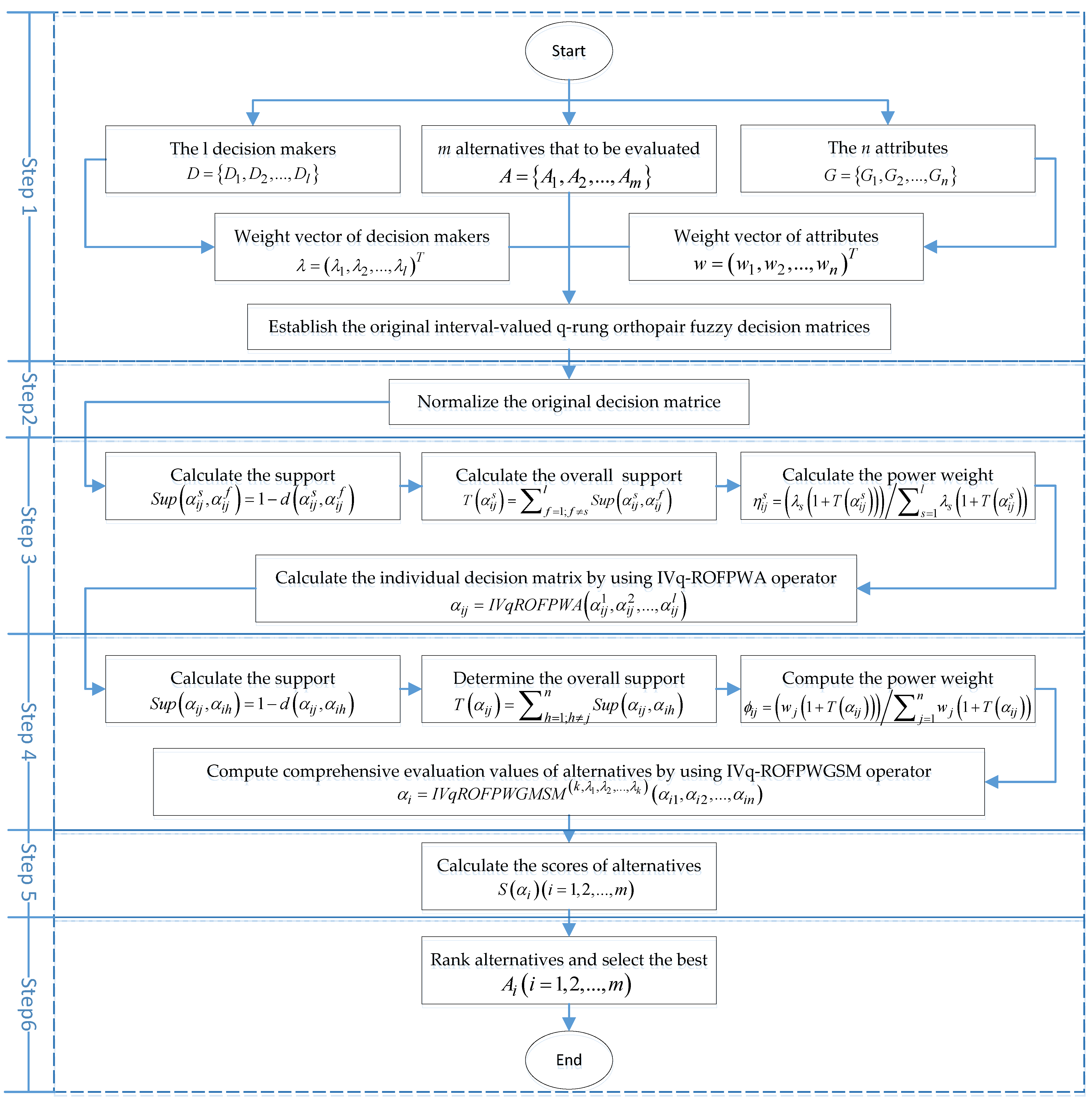
4. A New Multi-Attribute Group Decision-Making Method Based on Interval-Valued q-Rung Orthopair Fuzzy Numbers

This section investigates a new MAGDM method under IVq-ROFSs. We assume there are m alternatives to be evaluated, which can be denoted as $A=\left\{A_1,A_2,\dots ,A_m\right\}$. There are l decision-makers that are asked to evaluate the performance of the candidates. The group of decision-makers can be denoted as $\left\{D_1,D_2,\dots ,D_l\right\}$. The weight vector of decision-makers is $\lambda ={\left({\lambda }_1,{\lambda }_2,\dots ,{\lambda }_l\right)}^T$, such that ${\sum }_{t=1}^l{\lambda }_t=1$ and $0\le {\lambda }_t\le 1$. Suppose that decision-makers are required to evaluate the alternatives under n attributes, and the attribute set can be expressed as $G={\left(G_1,G_2,\dots ,G_n\right)}^T$. Weight vector of these attributes is $w={\left(w_1,w_2,\dots ,w_n\right)}^T$, satisfying ${\sum }_{j=1}^n{w}_j=1$ and $0\le w_j\le 1$. In the following, we present a novel method to determine the optimal alternative.

Step 1. Construct the original decision matrices. Decision-makers are asked for evaluating the properties of the candidates under the n attributes by using IVq-ROFNs. For instance, decision-maker $D_t$ uses an IVq-ROFN ${\alpha }_{ij}^t=([a_{ij}^t,b_{ij}^t],[c_{ij}^t,d_{ij}^t])$ to express his/her evaluation value of the attribute $G_j\left(j=1,2,\dots ,n\right)$ of alternative $A_i\left(i=1,2,\dots ,m\right)$. Afterwards, a series of interval-valued q-rung orthopair fuzzy decision matrices are obtained.

Step 2. Normalize the original decision matrices. Considering the fact that there exist two kinds of attributes, i.e., benefit type (T₁) and cost type (T₂), the original decision matrices provided by decision-makers should be normalized according to the following formula, i.e.,

$${\alpha }_{ij}^t=\{\begin{array}{c}([a_{ij}^t,b_{ij}^t],[c_{ij}^t,d_{ij}^t]) for G_j\in T_1\\ ([c_{ij}^t,d_{ij}^t],[a_{ij}^t,b_{ij}^t]) for G_j\in T_2\end{array}$$

(39)

Step 3. Determine the comprehensive decision matrix.

Step 3.1. Calculate the support $Sup({\alpha }_{ij}^s,{\alpha }_{ij}^f)$ by

$$Sup({\alpha }_{ij}^s,{\alpha }_{ij}^f)=1-d({\alpha }_{ij}^s,{\alpha }_{ij}^f),$$

(40)

where $s,f=1,2,\dots ,l(s\ne f)$ and $d({\alpha }_{ij}^s,{\alpha }_{ij}^f)$ denotes the distance between ${\alpha }_{ij}^s$ and ${\alpha }_{ij}^f$.

Step 3.2. Calculate the overall support $T({\alpha }_{ij}^s)$ by

$$T({\alpha }_{ij}^s)={\sum }_{f=1,f\ne s}^{l}Sup({\alpha }_{ij}^s,{\alpha }_{ij}^f),$$

(41)

Step 3.3. Compute the power weight associated with ${\alpha }_{ij}^s$ by

$${\eta }_{ij}^s=\frac{{\lambda }_s(1+T({\alpha }_{ij}^s))}{{\sum }_{s=1}^l{\lambda }_s(1+T({\alpha }_{ij}^s))},$$

(42)

Step 3.4. Utilize the IVq-ROFPWA operator to compute the overall decision matrix, i.e.,

$${\alpha }_{ij}=IVqROFPWA({\alpha }_{ij}^1,{\alpha }_{ij}^2,\dots ,{\alpha }_{ij}^l),$$

(43)

Step 4. Compute the overall evaluation value for each alternative.

Step 4.1. Calculate the support $Sup({\alpha }_{ij},{\alpha }_{ih})$ by

$$Sup({\alpha }_{ij},{\alpha }_{ih})=1-d({\alpha }_{ij},{\alpha }_{ih}),$$

(44)

where $j,h=1,2,\dots ,n(j\ne h)$ and $d({\alpha }_{ij},{\alpha }_{ih})$ is the distance between ${\alpha }_{ij}$ and ${\alpha }_{ih}$.

Step 4.2. Determine the overall support

$$T({\alpha }_{ij})={\sum }_{h=1,h\ne j}^{n}Sup({\alpha }_{ij},{\alpha }_{ih}),$$

(45)

Step 4.3. Compute the power weight of ${\alpha }_{ij}$ by

$${\varphi }_{ij}=\frac{w_j(1+T({\alpha }_{ij}))}{{\sum }_{j=1}^n{w}_j(1+T({\alpha }_{ij}))},$$

(46)

Step 4.4. Obtain the overall evaluation values by using the IVq-ROFPWGMSM operator, i.e.,

$${\alpha }_i=IVqROFPWGMS{M}^{(k,{\lambda }_1,{\lambda }_2,\dots ,{\lambda }_k)}({\alpha }_{i1},{\alpha }_{i2},\dots ,{\alpha }_{in}),$$

(47)

Step 5. Compute the score values of alternatives $X_i(i=1,2,\dots ,m)$.

Step 6. Determine the rank of their scores and choose the best one.

To better demonstrate the steps of our new proposed MAGDM method, we provide the following Figure 1.

5. An Application of the Proposed Method in Online Education Platform Performance Evaluation

With the rise of the Internet, the education industry has ushered in new development opportunities, and increasingly more online education platforms have sprung up. Mobile Internet and 5G communication technology have promoted the development of the online education industry, and the development of online education platforms is showing a blowout trend. In addition, affected by COVID-19, more and more schools and educational institutions adopt online teaching models, which objectively promotes the development of online education platforms. Online teaching platforms cannot only realize distance teaching, but are also considered to be an important measure to promote the flow and reasonable distribution of teaching resources, and can alleviate the structural contradictions caused by the unbalanced distribution of educational resources. Therefore, all countries are vigorously developing online education platforms. With the continuous increase in the number of online education platforms, their uneven quality has also received widespread attention from the public. Therefore, it is very necessary to evaluate the performance of online education platforms. Assume that three decision-makers (D₁, D₂, and D₃) are invited to evaluate the performance of four famous online education platforms, which can be denoted as A₁, A₂, A₃, and A_4. Weight vector of decision-maker is $\lambda ={\left(0.3,0.3,0.4\right)}^T$. Decision-makers evaluate the performance of the four education platforms under four attributes, i.e., availability (G₁), interactive quality (G₂), system quality (G₃), and quality of service (G₄). Weight vector of attributes is $w={\left(0.40,0.25,0.20,0.15\right)}^T$.

5.1. Online Education Platforms Performance Evaluation Process

Step 1. Require the three decision-makers to provide their evaluation values in the form of IVq-ROFNs. Hence, we can obtain three interval-valued q-rung orthopair fuzzy decision matrices, which are presented in

Table 1. The decision matrix provided D₁.

	G1	G2	G3	G4
A1	$\left(\left[0.3,0.6\right],\left[0.7,0.8\right]\right)$	$\left(\left[0.4,0.5\right],\left[0.6,0.8\right]\right)$	$\left(\left[0.5,0.6\right],\left[0.7,0.9\right]\right)$	$\left(\left[0.4,0.7\right],\left[0.6,0.7\right]\right)$
A2	$\left(\left[0.2,0.3\right],\left[0.7,0.9\right]\right)$	$\left(\left[0.2,0.5\right],\left[0.6,0.9\right]\right)$	$\left(\left[0.4,0.6\right],\left[0.8,0.9\right]\right)$	$\left(\left[0.2,0.4\right],\left[0.6,0.8\right]\right)$
A3	$\left(\left[0.3,0.4\right],\left[0.5,0.7\right]\right)$	$\left(\left[0.4,0.5\right],\left[0.6,0.8\right]\right)$	$\left(\left[0.1,0.2\right],\left[0.6,0.7\right]\right)$	$\left(\left[0.1,0.3\right],\left[0.7,0.8\right]\right)$
A4	$\left(\left[0.1,0.2\right],\left[0.7,0.9\right]\right)$	$\left(\left[0.3,0.5\right],\left[0.6,0.8\right]\right)$	$\left(\left[0.4,0.5\right],\left[0.5,0.6\right]\right)$	$\left(\left[0.3,0.5\right],\left[0.7,0.9\right]\right)$

,

Table 2. The decision matrix provided D₂.

	G1	G2	G3	G4
A1	$\left(\left[0.2,0.4\right],\left[0.6,0.7\right]\right)$	$\left(\left[0.3,0.6\right],\left[0.8,0.9\right]\right)$	$\left(\left[0.1,0.3\right],\left[0.6,0.9\right]\right)$	$\left(\left[0.3,0.4\right],\left[0.6,0.7\right]\right)$
A2	$\left(\left[0.1,0.2\right],\left[0.8,0.9\right]\right)$	$\left(\left[0.5,0.6\right],\left[0.7,0.8\right]\right)$	$\left(\left[0.2,0.4\right],\left[0.6,0.7\right]\right)$	$\left(\left[0.1,0.3\right],\left[0.7,0.9\right]\right)$
A3	$\left(\left[0.3,0.5\right],\left[0.8,0.9\right]\right)$	$\left(\left[0.3,0.4\right],\left[0.7,0.9\right]\right)$	$\left(\left[0.2,0.4\right],\left[0.5,0.8\right]\right)$	$\left(\left[0.2,0.3\right],\left[0.6,0.8\right]\right)$
A4	$\left(\left[0.3,0.4\right],\left[0.6,0.8\right]\right)$	$\left(\left[0.1,0.2\right],\left[0.7,0.9\right]\right)$	$\left(\left[0.2,0.3\right],\left[0.6,0.7\right]\right)$	$\left(\left[0.6,0.7\right],\left[0.3,0.5\right]\right)$

and

Table 3. The decision matrix provided D₃.

	G1	G2	G3	G4
A1	$\left(\left[0.1,0.2\right],\left[0.5,0.7\right]\right)$	$\left(\left[0.2,0.4\right],\left[0.5,0.6\right]\right)$	$\left(\left[0.3,0.4\right],\left[0.2,0.4\right]\right)$	$\left(\left[0.3,0.5\right],\left[0.2,0.4\right]\right)$
A2	$\left(\left[0.1,0.2\right],\left[0.5,0.7\right]\right)$	$\left(\left[0.2,0.4\right],\left[0.4,0.5\right]\right)$	$\left(\left[0.3,0.4\right],\left[0.5,0.7\right]\right)$	$\left(\left[0.2,0.3\right],\left[0.4,0.5\right]\right)$
A3	$\left(\left[0.5,0.8\right],\left[0.1,0.2\right]\right)$	$\left(\left[0.4,0.5\right],\left[0.7,0.8\right]\right)$	$\left(\left[0.2,0.4\right],\left[0.6,0.8\right]\right)$	$\left(\left[0.6,0.8\right],\left[0.1,0.2\right]\right)$
A4	$\left(\left[0.5,0.6\right],\left[0.2,0.3\right]\right)$	$\left(\left[0.6,0.8\right],\left[0.3,0.4\right]\right)$	$\left(\left[0.5,0.7\right],\left[0.4,0.5\right]\right)$	$\left(\left[0.2,0.5\right],\left[0.6,0.8\right]\right)$

.

Step 2. Normalize the original decision matrices. It is noted that all attributes are benefit type and hence the original decision matrices do not need to be normalized.

Step 3. Determine the integrated decision matrix.

Step 3.1. According to Equation (40), calculate the values $Sup({\alpha }_{ij}^s,{\alpha }_{ij}^f)$. Hence, we can obtain the following results

$$\begin{array}{c}Su{p}^{\left(1,2\right)}=Su{p}^{\left(2,1\right)}=\left[\begin{array}{ccc}0.8833& 0.8398& \begin{array}{cc}0.8900& 0.9210\end{array}\\ 0.9512& 0.8620& \begin{array}{cc}0.7775& 0.9030\end{array}\\ \begin{array}{c}0.7915\\ 0.8935\end{array}& \begin{array}{c}0.8895\\ 0.8783\end{array}& \begin{array}{cc}\begin{array}{c}0.9192\\ 0.9070\end{array}& \begin{array}{c}0.9665\\ 0.6683\end{array}\end{array}\end{array}\right]\\ Su{p}^{\left(1,3\right)}=Su{p}^{\left(3,1\right)}=\left[\begin{array}{ccc}0.8448& 0.8740& \begin{array}{cc}0.6875& 0.8145\end{array}\\ 0.8425& 0.7958& \begin{array}{cc}0.7595& 0.8560\end{array}\\ \begin{array}{c}0.7488\\ 0.6578\end{array}& \begin{array}{c}0.9683\\ 0.6968\end{array}& \begin{array}{cc}\begin{array}{c}0.9420\\ 0.8923\end{array}& \begin{array}{c}0.6135\\ 0.9093\end{array}\end{array}\end{array}\right]\\ Su{p}^{\left(2,3\right)}=Su{p}^{\left(3,2\right)}=\left[\begin{array}{ccc}0.9615& 0.7323& \begin{array}{cc}0.7660& 0.8630\end{array}\\ 0.8067& 0.7663& \begin{array}{cc}0.9725& 0.7775\end{array}\\ \begin{array}{c}0.5707\\ 0.7643\end{array}& \begin{array}{c}0.9213\\ 0.5750\end{array}& \begin{array}{cc}\begin{array}{c}0.9773\\ 0.7993\end{array}& \begin{array}{c}0.6470\\ 0.7495\end{array}\end{array}\end{array}\right]\end{array}$$

It is noted that we use the symbol $Su{p}^{\left(s,f\right)}$ to denote the supports of ${\alpha }_{ij}^s$ from ${\alpha }_{ij}^f$, where $s,f=1,2,3$ and $s\ne f$.

Step 3.2. Calculate the overall support $T\left({\alpha }_{ij}^s\right)$ by Equation (41) and we can obtain

$$\begin{array}{c}{T}^{\left(1\right)}=\left[\begin{array}{ccc}1.7280& 1.7138& \begin{array}{cc}1.5775& 1.7355\end{array}\\ 1.7938& 1.6578& \begin{array}{cc}1.5370& 1.7590\end{array}\\ \begin{array}{c}1.5403\\ 1.5513\end{array}& \begin{array}{c}1.8578\\ 1.5750\end{array}& \begin{array}{cc}\begin{array}{c}1.8612\\ 1.7993\end{array}& \begin{array}{c}1.5800\\ 1.5775\end{array}\end{array}\end{array}\right]\\ T^{\left(2\right)}=\left[\begin{array}{ccc}1.8448& 1.5720& \begin{array}{cc}1.6560& 1.7840\end{array}\\ 1.7580& 1.6283& \begin{array}{cc}1.7500& 1.6805\end{array}\\ \begin{array}{c}1.3622\\ 1.6578\end{array}& \begin{array}{c}1.8108\\ 1.4533\end{array}& \begin{array}{cc}\begin{array}{c}1.8965\\ 1.7063\end{array}& \begin{array}{c}1.6135\\ 1.4178\end{array}\end{array}\end{array}\right]\\ T^{\left(3\right)}=\left[\begin{array}{ccc}1.8063& 1.6063& \begin{array}{cc}1.4535& 1.6775\end{array}\\ 1.6492& 1.5620& \begin{array}{cc}1.7320& 1.6335\end{array}\\ \begin{array}{c}1.3195\\ 1.4220\end{array}& \begin{array}{c}1.8895\\ 1.2718\end{array}& \begin{array}{cc}\begin{array}{c}1.9193\\ 1.6915\end{array}& \begin{array}{c}1.2605\\ 1.6588\end{array}\end{array}\end{array}\right]\end{array}$$

Here we use the symbol $T^{\left(s\right)}$ to represent the overall supports for ${\alpha }_{ij}^s$, where $s=1,2,3$.

Step 3.3. Compute the power weight associated with ${\alpha }_{ij}^s$ by Equation (42) and we have

$$\begin{array}{c}{\eta }^{\left(1\right)}=\left[\begin{array}{ccc}0.2929& 0.3098& \begin{array}{cc}0.3031& 0.3010\end{array}\\ 0.3075& 0.3054& \begin{array}{cc}0.2841& 0.3082\end{array}\\ \begin{array}{c}0.3177\\ 0.3023\end{array}& \begin{array}{c}0.3001\\ 0.3196\end{array}& \begin{array}{cc}\begin{array}{c}0.2965\\ 0.3078\end{array}& \begin{array}{c}0.3143\\ 0.3018\end{array}\end{array}\end{array}\right]\\ {\eta }^{\left(2\right)}=\left[\begin{array}{ccc}0.3054& 0.2936& \begin{array}{cc}0.3123& 0.3063\end{array}\\ 0.3036& 0.3020& \begin{array}{cc}0.3080& 0.2995\end{array}\\ \begin{array}{c}0.2955\\ 0.3150\end{array}& \begin{array}{c}0.2952\\ 0.3045\end{array}& \begin{array}{cc}\begin{array}{c}0.3002\\ 0.2976\end{array}& \begin{array}{c}0.3184\\ 0.2831\end{array}\end{array}\end{array}\right]\\ {\eta }^{\left(3\right)}=\left[\begin{array}{ccc}0.4017& 0.3967& \begin{array}{cc}0.3846& 0.3928\end{array}\\ 0.3888& 0.3926& \begin{array}{cc}0.4079& 0.3923\end{array}\\ \begin{array}{c}0.3868\\ 0.3827\end{array}& \begin{array}{c}0.4046\\ 0.3759\end{array}& \begin{array}{cc}\begin{array}{c}0.4033\\ 0.3946\end{array}& \begin{array}{c}0.3672\\ 0.4151\end{array}\end{array}\end{array}\right]\end{array}$$

Here we use the symbol ${\eta }^{\left(s\right)}$ to denote the power weights associated with the IVq-ROFN ${\alpha }_{ij}^s$, where $s=1,2,3$.

Step 3.4. Use the IVq-ROFPWA operator to determine the integrated decision matrix, which is listed in

Table 4. The comprehensive decision matrix.

	G1	G2
A1	$\left(\left[0.0738,0.1477\right],\left[0.7570,0.8665\right]\right)$	$\left(\left[0.1471,0.2958\right],\left[0.7596,0.8166\right]\right)$
A2	$\left(\left[0.0730,0.1461\right],\left[0.7637,0.8705\right]\right)$	$\left(\left[0.1466,0.2948\right],\left[0.6979,0.7618\right]\right)$
A3	$\left(\left[0.3692,0.6235\right],\left[0.4104,0.5366\right]\right)$	$\left(\left[0.2978,0.3747\right],\left[0.8656,0.9137\right]\right)$
A4	$\left(\left[0.3680,0.4463\right],\left[0.5401,0.6308\right]\right)$	$\left(\left[0.4438,0.6183\right],\left[0.6360,0.7086\right]\right)$
	G3	G4
A1	$\left(\left[0.2188,0.2929\right],\left[0.5384,0.7030\right]\right)$	$\left(\left[0.2203,0.3711\right],\left[0.5315,0.6978\right]\right)$
A2	$\left(\left[0.2231,0.2986\right],\left[0.7537,0.8646\right]\right)$	$\left(\left[0.1465,0.2202\right],\left[0.6981,0.7619\right]\right)$
A3	$\left(\left[0.1479,0.2975\right],\left[0.8138,0.9139\right]\right)$	$\left(\left[0.4405,0.6141\right],\left[0.4293,0.5538\right]\right)$
A4	$\left(\left[0.3716,0.5346\right],\left[0.6966,0.7607\right]\right)$	$\left(\left[0.1493,0.3778\right],\left[0.8089,0.9115\right]\right)$

.

Step 4. Compute the overall evaluation value for each alternative.

Step 4.1. Calculate the support $Sup\left({\alpha }_{ij},{\alpha }_{ih}\right)$ by Equation (43)

$$\begin{array}{c}Su{p}_{1,2}=Su{p}_{2,1}=\left(0.9660,0.9129,0.6497,0.9026\right);\\ Su{p}_{1,3}=Su{p}_{3,1}=\left(0.8468,0.9838,0.6645,0.8913\right);\\ Su{p}_{1,4}=Su{p}_{4,1}=\left(0.8368,0.9168,0.9822,0.7601\right);\\ Su{p}_{2,3}=Su{p}_{3,2}=\left(0.8782,0.9246,0.9601,0.9288\right);\\ Su{p}_{2,4}=Su{p}_{4,2}=\left(0.8686,0.9961,0.6499,0.7649\right);\\ Su{p}_{3,4}=Su{p}_{4,3}=\left(0.9900,0.9210,0.6648,0.8362\right);\end{array}$$

Here we employ the symbol $Su{p}_{j,h}$ to denote the supports for ${\alpha }_{ij}$ from ${\alpha }_{ih}$, where $j,h=1,2,3,4$ and $j\ne h$.

Step 4.2. Determine the overall support $T\left({\alpha }_{ij}\right)$ by using Equation (44), and we have the following results.

$$T=\left[\begin{array}{ccc}2.6496& 2.7127& \begin{array}{cc}2.7150& 2.6954\end{array}\\ 2.8134& 2.8337& \begin{array}{cc}2.8295& 2.8339\end{array}\\ \begin{array}{c}2.2964\\ 2.5540\end{array}& \begin{array}{c}2.2596\\ 2.5963\end{array}& \begin{array}{cc}\begin{array}{c}2.2894\\ 2.6562\end{array}& \begin{array}{c}2.2969\\ 2.3612\end{array}\end{array}\end{array}\right]$$

Step 4.3. Compute the power weight of ${\alpha }_{ij}$ according to Equation (45) and we have

$$\varphi =\left[\begin{array}{ccc}0.3961& 0.2519& \begin{array}{cc}0.2016& 0.1504\end{array}\\ 0.3988& 0.2506& \begin{array}{cc}0.2002& 0.1504\end{array}\\ \begin{array}{c}0.4013\\ 0.3998\end{array}& \begin{array}{c}0.2480\\ 0.2528\end{array}& \begin{array}{cc}\begin{array}{c}0.2002\\ 0.2056\end{array}& \begin{array}{c}0.1505\\ 0.1418\end{array}\end{array}\end{array}\right]$$

Step 4.4. Obtain the overall evaluation values by using the IVq-ROFPWGMSM operator, then we have the following results, viz.,

$$\begin{array}{c}{\alpha }_1=\left(\left[0.1633,0.2708\right],\left[0.6766,0.7934\right]\right)\\ {\alpha }_2=\left(\left[0.1466,0.2390\right],\left[0.7433,0.8293\right]\right)\\ {\alpha }_3=\left(\left[0.3320,0.4984\right],\left[0.7085,0.7898\right]\right)\\ {\alpha }_4=\left(\left[0.3660,0.5030\right],\left[0.6984,0.7681\right]\right)\end{array}$$

Step 5. Compute the score values of alternatives $X_i\left(i=1,2,\dots ,m\right)$.

$$\begin{array}{c}S\left(A_1\right)=0.4487,\\ S\left(A_2\right)=0.4575,\\ S\left(A_3\right)=0.4440,\\ S\left(A_4\right)=0.4523\end{array}$$

Step 6. Determine the rank of alternatives and we can obtain $A_2\succ A_4\succ A_1\succ A_3$. Hence, $A_2$ is the best online education platform.

5.2. Parameter Analysis

It is noted that the parameters in our proposed MAGDM method have significant impact on the decision results. Hence, it is worth investigating the effect of the parameters on the decision results.

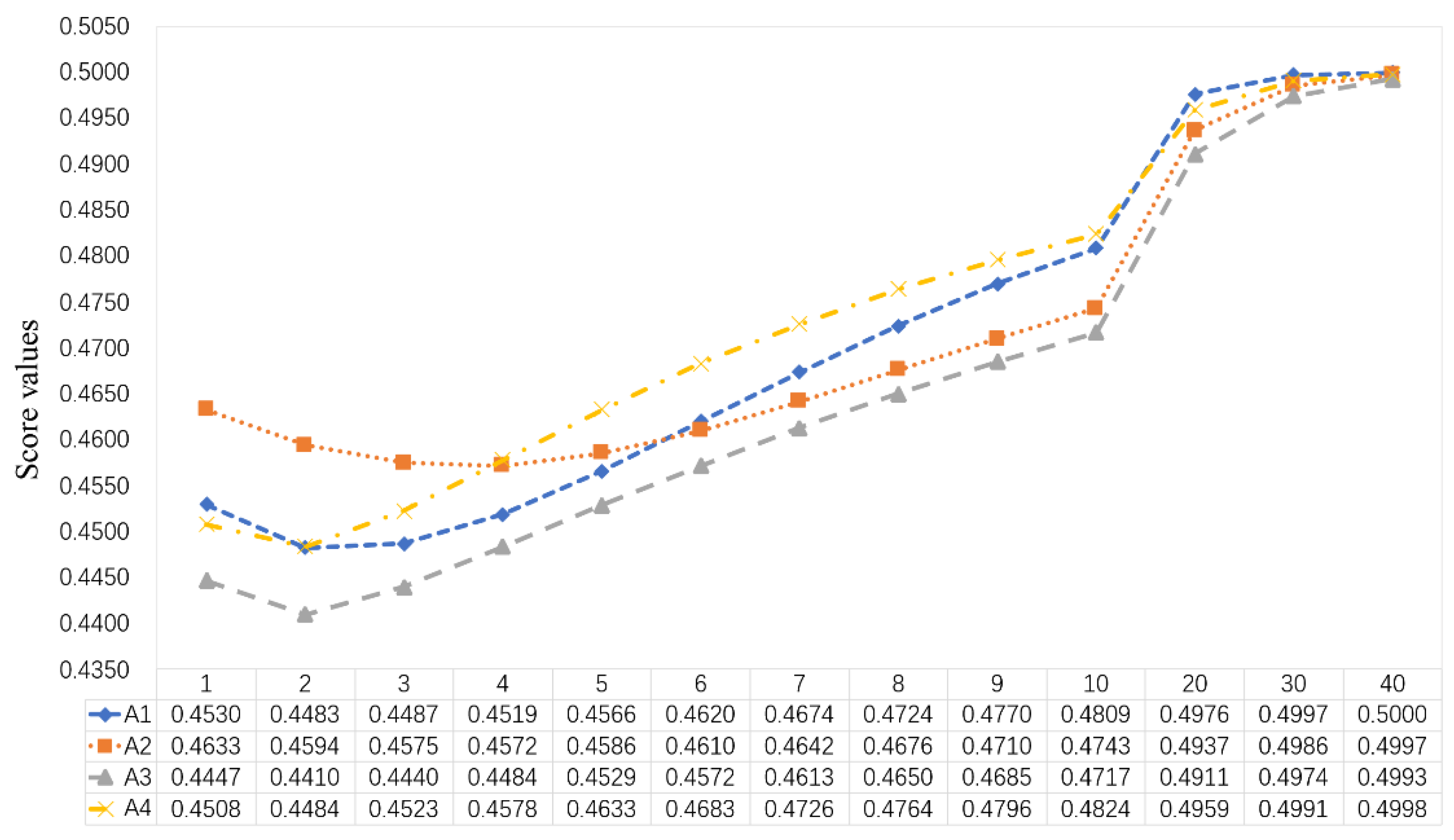
5.2.1. The Impact of q

We first investigate the influence of the parameter q on the decision results. We use different values of q in our MAGDM method and present the final decision results in

Table 5. Ranking results by the proposed method when $k=2,{\lambda }_1=1,{\lambda }_2=1$ for different values of the parameter q.

q	$\mathbf{Scores} \mathit{S}\left({\mathit{\alpha }}_{\mathit{i}}\right)\left(\mathit{i}=1,2,3,4\right)$	Ranking Orders
q = 1	$S\left({\alpha }_1\right)=$0.4530, $S\left({\alpha }_2\right)=0.4633$, $S\left({\alpha }_3\right)=0.4447$, $S\left({\alpha }_4\right)=0.4508$	$A_2\succ A_1\succ A_4\succ A_3$
q = 2	$S\left({\alpha }_1\right)=0.4483$, $S\left({\alpha }_2\right)=0.4594$, $S\left({\alpha }_3\right)=0.4410$, $S\left({\alpha }_4\right)=0.4484$	$A_2\succ A_4\succ A_1\succ A_3$
q = 3	$S\left({\alpha }_1\right)=0.4487$,$S\left({\alpha }_2\right)=0.4575$, $S\left({\alpha }_3\right)=0.4440$, $S\left({\alpha }_4\right)=0.4523$	$A_2\succ A_4\succ A_1\succ A_3$
q = 4	$S\left({\alpha }_1\right)=0.4519$, $S\left({\alpha }_2\right)=0.4572$, $S\left({\alpha }_3\right)=0.4484$,$S\left({\alpha }_4\right)=0.4578$	$A_4\succ A_2\succ A_1\succ A_3$
q = 5	$S\left({\alpha }_1\right)=0.4566$, $S\left({\alpha }_2\right)=0.4586$, $S\left({\alpha }_3\right)=0.4529$,$S\left({\alpha }_4\right)=0.4633$	$A_4\succ A_2\succ A_1\succ A_3$
q = 6	$S\left({\alpha }_1\right)=0.4620$, $S\left({\alpha }_2\right)=0.4610$, $S\left({\alpha }_3\right)=0.4572$, $S\left({\alpha }_4\right)=0.4683$	$A_4\succ A_2\succ A_1\succ A_3$
q = 7	$S\left({\alpha }_1\right)=0.4674$, $S\left({\alpha }_2\right)=0.4642$, $S\left({\alpha }_3\right)=0.4613$, $S\left({\alpha }_4\right)=0.4726$	$A_4\succ A_2\succ A_1\succ A_3$
q = 8	$S\left({\alpha }_1\right)=0.4724$, $S\left({\alpha }_2\right)=0.4676$,$S\left({\alpha }_3\right)=0.4650$, $S\left({\alpha }_4\right)=0.4764$	$A_4\succ A_2\succ A_1\succ A_3$
q = 9	$S\left({\alpha }_1\right)=0.4770$, $S\left({\alpha }_2\right)=0.4710$, $S\left({\alpha }_3\right)=0.4685$, $S\left({\alpha }_4\right)=0.4796$	$A_4\succ A_2\succ A_1\succ A_3$
q = 10	$S\left({\alpha }_1\right)=0.4809$, $S\left({\alpha }_2\right)=0.4743$, $S\left({\alpha }_3\right)=0.4717$, $S\left({\alpha }_4\right)=0.4824$	$A_4\succ A_2\succ A_1\succ A_3$
q = 20	$S\left({\alpha }_1\right)=0.4976$, $S\left({\alpha }_2\right)=0.4937$, $S\left({\alpha }_3\right)=0.4911$, $S\left({\alpha }_4\right)=0.4959$	$A_1\succ A_4\succ A_2\succ A_3$
q = 30	$S\left({\alpha }_1\right)=0.4997$, $S\left({\alpha }_2\right)=0.4986$, $S\left({\alpha }_3\right)=0.4974$, $S\left({\alpha }_4\right)=0.4991$	$A_1\succ A_4\succ A_2\succ A_3$
q = 40	$S\left({\alpha }_1\right)=0.5000$, $S\left({\alpha }_2\right)=0.4997$, $S\left({\alpha }_3\right)=0.4993$, $S\left({\alpha }_4\right)=0.4998$	$A_1\succ A_4\succ A_2\succ A_3$

. In addition, we also provide Figure 2 to better illustrate the decision-making results.

It is noted that when the variables k and $\lambda$ remain unchanged, with the increase in the value of q, all the results show a trend of decreasing firstly and increasing afterwards. When the value of q is small, the result value decreases gradually with the increase in q. When the value of q is large, the result value gradually increases with the increase in q. In addition, different q values lead to different sorting results but $A_3$ is always the worst alternative, whereas the optimal alternative keeps in changing. More specifically, $A_2$ is the optimal alternative when $q=1$, 2 and 3. If $q=4$ or 10, the optimal alternative is $A_4$. Hence, the value of q has significant impact on the decision results. In practical MAGDM problems, decision-makers can choose a proper value of q according to evaluation values provided by decision-makers. The principle of determining the value of q is that its should take the smallest integer that satisfies the constraint $b^q+d^q\le 1$. For instance, if the attribute value is $\left[\left(0.6,0.9\right),\left(0.7,0.8\right)\right]$, then the value can be taken as ${0.9}^4+{0.8}^4=1.0657>1$ and ${0.9}^5+{0.8}^5=0.91817<1$, hence, the value of q is 5.

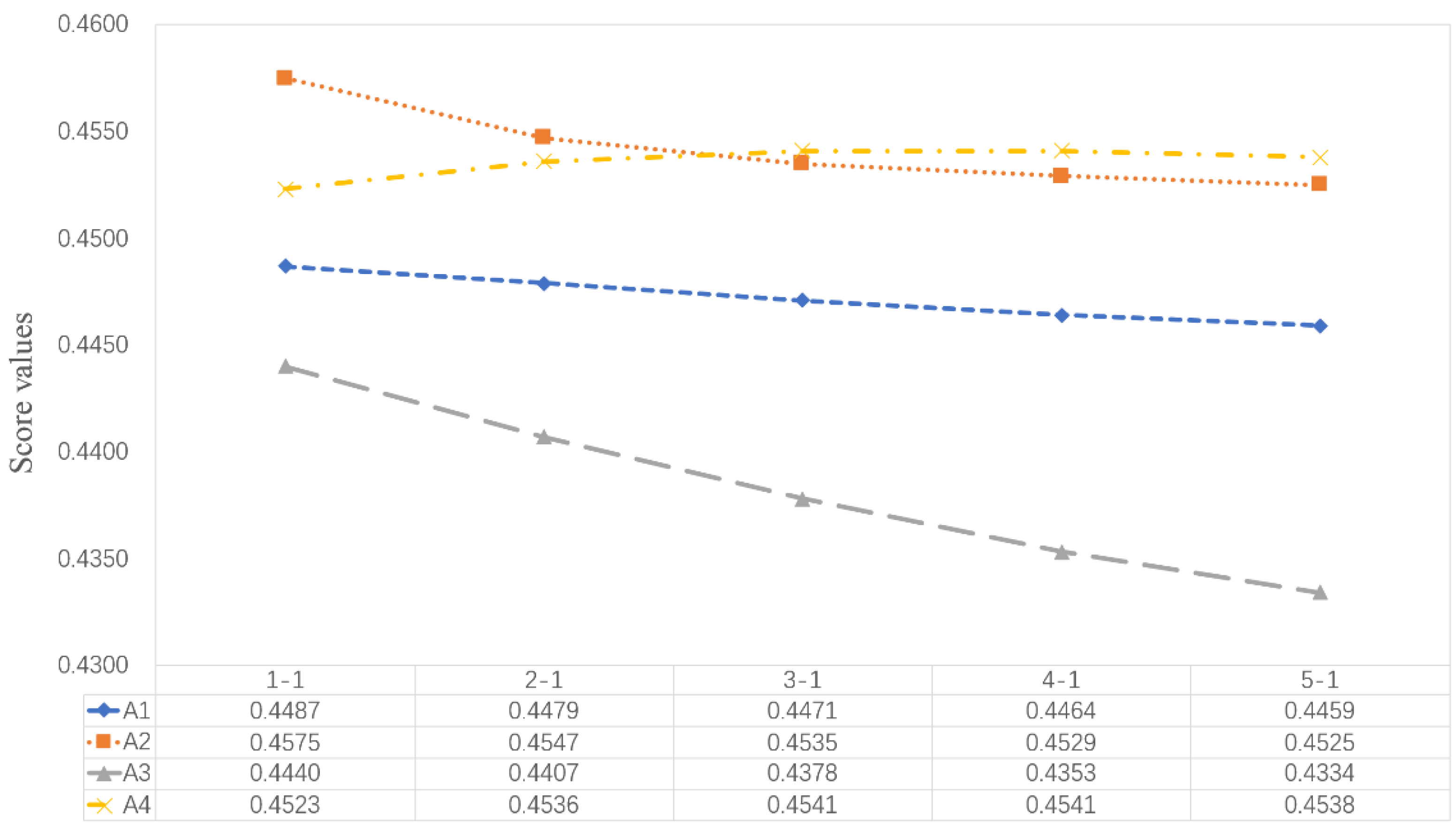
5.2.2. The Impact of $\mathsf{\lambda }$

In order to evaluate the impact of different λ on the final evaluation results, we keep k and q unchanged and use different λ in the IVq-ROFPWGMSM operator to determine the final decision results. The corresponding results are shown in

Table 6. Ranking results by the proposed method when q = 3, k = 2 for different values of the parameter ${\lambda }_1$ and ${\lambda }_2$.

${\mathit{\lambda }}_1$	${\mathit{\lambda }}_2$	$\mathbf{Score} \mathbf{Values} \mathit{S}\left({\mathit{\alpha }}_{\mathit{i}}\right)\left(\mathit{i}=1,2,3,4\right)$	Ranking Orders
${\lambda }_1=1$	${\lambda }_2=1$	$S\left({\alpha }_1\right)=0.4487$, $S\left({\alpha }_2\right)=0.4575$, $S\left({\alpha }_3\right)=0.4440$, $S\left({\alpha }_4\right)=0.4523$	$A_2\succ A_4\succ A_1\succ A_3$
${\lambda }_1=1$	${\lambda }_2=2$	$S\left({\alpha }_1\right)=0.4484$, $S\left({\alpha }_2\right)=0.4607$, $S\left({\alpha }_3\right)=0.4464$, $S\left({\alpha }_4\right)=0.4544$	$A_2\succ A_4\succ A_1\succ A_3$
${\lambda }_1=1$	${\lambda }_2=3$	$S\left({\alpha }_1\right)=0.4480$, $S\left({\alpha }_2\right)=0.4629$, $S\left({\alpha }_3\right)=0.4477$, $S\left({\alpha }_4\right)=0.4548$	$A_2\succ A_4\succ A_1\succ A_3$
${\lambda }_1=1$	${\lambda }_2=4$	$S\left({\alpha }_1\right)=0.4476$, $S\left({\alpha }_2\right)=0.4647$, $S\left({\alpha }_3\right)=0.4484$, $S\left({\alpha }_4\right)=0.4542$	$A_2\succ A_4\succ A_1\succ A_3$
${\lambda }_1=1$	${\lambda }_2=5$	$S\left({\alpha }_1\right)=0.4474$,$S\left({\alpha }_2\right)=0.4663$,$S\left({\alpha }_3\right)=0.4485$,$S\left({\alpha }_4\right)=0.4532$	$A_2\succ A_4\succ A_3\succ A_1$
${\lambda }_1=2$	${\lambda }_2=1$	$S\left({\alpha }_1\right)=0.4479$, $S\left({\alpha }_2\right)=0.4547$, $S\left({\alpha }_3\right)=0.4407$, $S\left({\alpha }_4\right)=0.4536$	$A_2\succ A_4\succ A_1\succ A_3$
${\lambda }_1=3$	${\lambda }_2=1$	$S\left({\alpha }_1\right)=0.4471$, $S\left({\alpha }_2\right)=0.4535$, $S\left({\alpha }_3\right)=0.4378$, $S\left({\alpha }_4\right)=0.4541$	$A_4\succ A_2\succ A_1\succ A_3$
${\lambda }_1=4$	${\lambda }_2=1$	$S\left({\alpha }_1\right)=0.4464$, $S\left({\alpha }_2\right)=0.4529$, $S\left({\alpha }_3\right)=0.4353$, $S\left({\alpha }_4\right)=0.4541$	$A_4\succ A_2\succ A_1\succ A_3$
${\lambda }_1=5$	${\lambda }_2=1$	$S\left({\alpha }_1\right)=0.4459$, $S\left({\alpha }_2\right)=0.4525$, $S\left({\alpha }_3\right)=0.4334$, $S\left({\alpha }_4\right)=0.4538$	$A_4\succ A_2\succ A_1\succ A_3$
${\lambda }_1=0.5$	${\lambda }_2=0.5$	$S\left({\alpha }_1\right)=0.4491$, $S\left({\alpha }_2\right)=0.4574$, $S\left({\alpha }_3\right)=0.4436$, $S\left({\alpha }_4\right)=0.4494$	$A_2\succ A_4\succ A_1\succ A_3$
${\lambda }_1=2$	${\lambda }_2=2$	$S\left({\alpha }_1\right)=0.4481$, $S\left({\alpha }_2\right)=0.4576$, $S\left({\alpha }_3\right)=0.4444$, $S\left({\alpha }_4\right)=0.4556$	$A_2\succ A_4\succ A_1\succ A_3$
${\lambda }_1=3$	${\lambda }_2=3$	$S\left({\alpha }_1\right)=0.4475$, $S\left({\alpha }_2\right)=0.4576$, $S\left({\alpha }_3\right)=0.4449$, $S\left({\alpha }_4\right)=0.4570$	$A_2\succ A_4\succ A_1\succ A_3$
${\lambda }_1=4$	${\lambda }_2=4$	$S\left({\alpha }_1\right)=0.4455$, $S\left({\alpha }_2\right)=0.4566$, $S\left({\alpha }_3\right)=0.4448$, $S\left({\alpha }_4\right)=0.4576$	$A_4\succ A_2\succ A_1\succ A_3$
${\lambda }_1=5$	${\lambda }_2=5$	$S\left({\alpha }_1\right)=0.4448$, $S\left({\alpha }_2\right)=0.4614$, $S\left({\alpha }_3\right)=0.4444$, $S\left({\alpha }_4\right)=0.4578$	$A_2\succ A_4\succ A_1\succ A_3$

. For the sake of easy description, we divide the researches into three groups to comprehensively analyze the influence of the parameters on the decision results. The decision-making results of each group are in Figure 3, Figure 4 and Figure 5.

First, we assume ${\lambda }_1$ to be a constant (${\lambda }_1=1$) and investigate how the parameter ${\lambda }_2$ affects the decision results. In Figure 3, we discover that when the value ${\lambda }_2$ increases, the score values of $A_2$ and $A_3$ also increase. In addition, the score values of $A_1$ decreases. The change in score values of $A_4$ is special. With the increase in value ${\lambda }_2$, the score value of $A_4$ increases at the beginning and decreases soon afterwards. Moreover, different values of ${\lambda }_2$ lead to different score values and ranking orders of alternatives. Nevertheless, the optimal alternative is always $A_2$.

Second, we assume ${\lambda }_2$ to be a constant (${\lambda }_2=1$) and study the influence the parameter ${\lambda }_1$ on the decision results. It can be seen from Figure 4 that the increase in value ${\lambda }_1$ leads the increase of the score values of $A_1$, $A_2$, and $A_3$. The change in the score value of $A_4$ is special. With the increase in the value ${\lambda }_1$, the score value of $A_4$ decreases first and increases afterwards. In addition, different values of ${\lambda }_1$ in the IVq-ROFPWGMSM operator result in different score values and ranking orders of alternatives. Moreover, the worst alternative is always $A_4$.

Third, we investigate the influence of the parameters ${\lambda }_1$ and ${\lambda }_2$ on the final decision results simultaneously (we assume ${\lambda }_1={\lambda }_2$). As seen from Figure 5, with the increase in values ${\lambda }_1$ and ${\lambda }_2$, some score value also increase and some other decrease. In addition, different values of parameters ${\lambda }_1$ and ${\lambda }_2$ lead to different score values and the worst optimal alternative is always $A_3$. From the above analysis, we can discover that the values of parameters ${\lambda }_1,{\lambda }_2,\dots ,{\lambda }_k$ have significant impact on the final decision results.

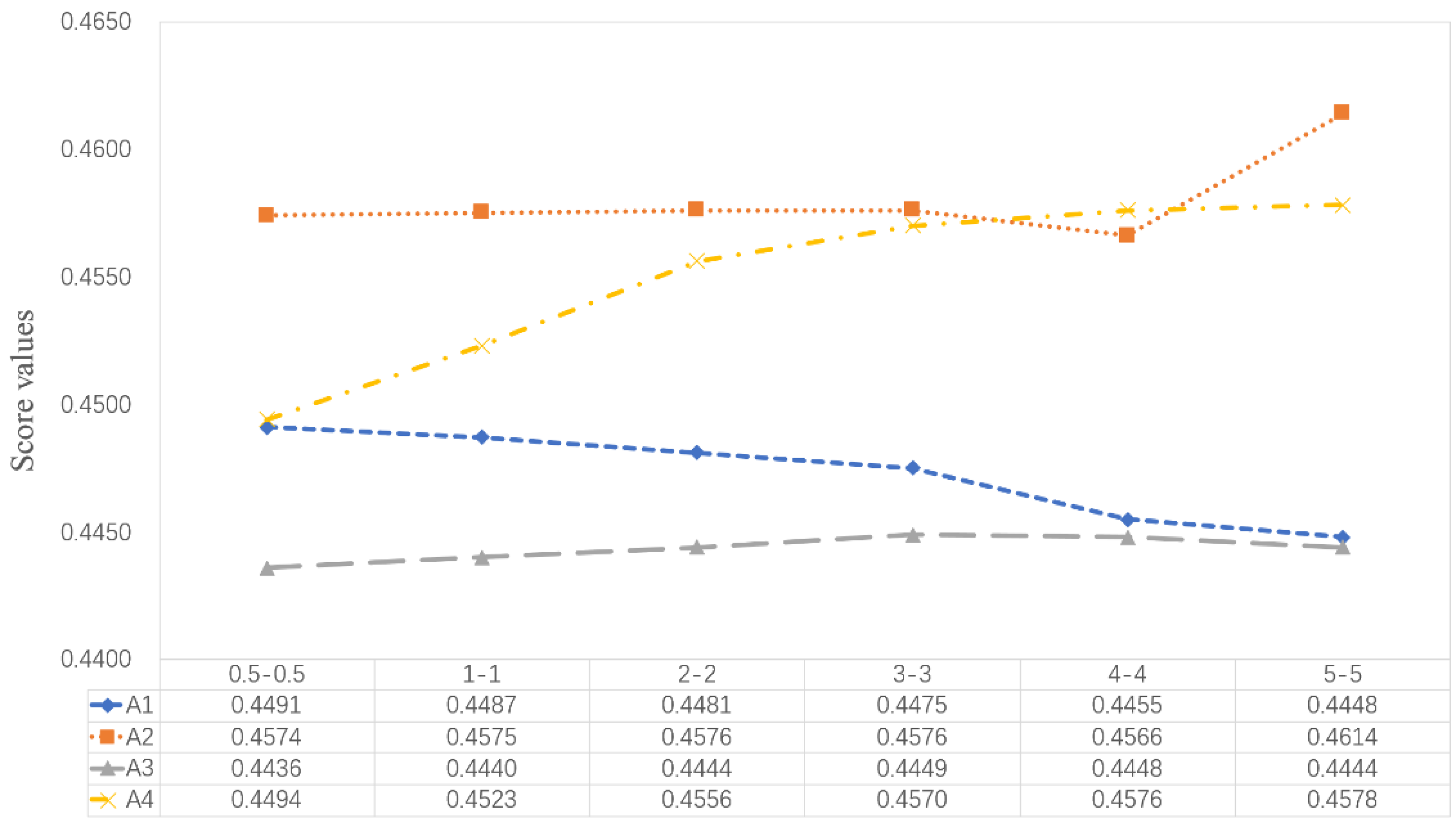
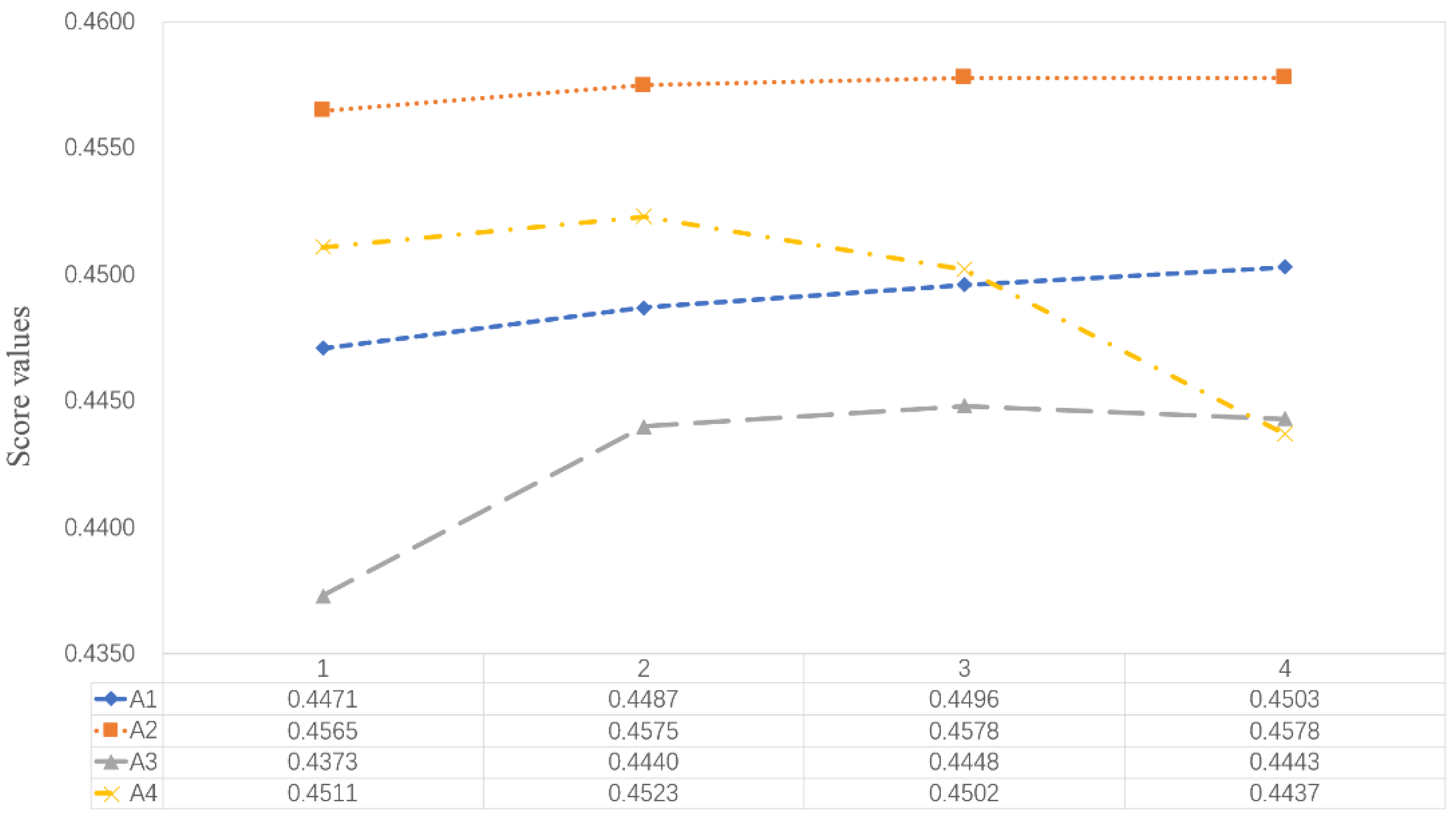
5.2.3. The Impact of k

In the following, we continue to investigate the influence of the parameter k on the decision results. We use different values of k in our proposed method and present the decision results in

Table 7. Ranking results by the proposed method when $q=3,{\lambda }_1={\lambda }_2=\cdots ={\lambda }_k=1$ for different values of the parameter k.

k	$\mathbf{Score} \mathbf{Values} \mathit{S}\left({\mathit{\alpha }}_{\mathit{i}}\right)\left(\mathit{i}=1,2,3,4\right)$	Ranking Orders
k = 1	$S\left({\alpha }_1\right)=$0.4471, $S\left({\alpha }_2\right)=0.4565$, $S\left({\alpha }_3\right)=0.4373$, $S\left({\alpha }_4\right)=0.4511$	$A_2\succ A_4\succ A_1\succ A_3$
k = 2	$S\left({\alpha }_1\right)=0.4487$, $S\left({\alpha }_2\right)=0.4575$, $S\left({\alpha }_3\right)=0.4440$, $S\left({\alpha }_4\right)=0.4523$	$A_2\succ A_4\succ A_1\succ A_3$
k = 3	$S\left({\alpha }_1\right)=0.4496$, $S\left({\alpha }_2\right)=0.4578$, $S\left({\alpha }_3\right)=0.4448$, $S\left({\alpha }_4\right)=0.4502$	$A_2\succ A_4\succ A_1\succ A_3$
k = 4	$S\left({\alpha }_1\right)=0.4503$, $S\left({\alpha }_2\right)=0.4578$, $S\left({\alpha }_3\right)=0.4443$, $S\left({\alpha }_4\right)=0.4437$	$A_2\succ A_1\succ A_3\succ A_4$

and Figure 6.

Figure 6 shows the score values and ranking orders of alternatives with different values of k in the IVq-ROFPWGMSM operator, when $q=3$ and ${\lambda }_1={\lambda }_2=\cdots ={\lambda }_k=1$. It is easy to find out that different score values and ranking orders of alternatives are obtained when we use different values of k in the IVq-ROFPWGMSM operator. Hence, it is necessary to determine a proper value of k. Basically, when $k=1$, our proposed method does not consider the interrelationship between attributes. When k = 2 or k = 3, then our method has the capability of capturing the interrelationship among any two or three attributes. In addition, when $k=4$, then our method takes the interrelationship among all the four attributes into account. Therefore, the proposed novel MAGDM method is effective for its ability to capture the interrelationship among attributes and it is suitable for handling realistic MAGDM problems, as in most decision-making problems attributes are usually interrelated. In MAGDM problems, decision-makers can determine a proper value of k according to actual needs.

5.3. Comparison Analysis

This subsection conducts comparison analysis. Through comparison analysis, the advantages and merits of our proposed method can be better demonstrated.

5.3.1. Compared with Power Bonferroni Mean Based Decision-Making Method

First of all, we compare our method with that based on the PBM operator. More specifically, we compare our proposed method with that developed by Liu and Li [32] based on the interval-valued intuitionistic fuzzy weighted power Bonferroni mean (IVIFWPBM) operator. We use both Liu and Li’s [32] method and our proposed method to solve the air quality evaluation problem presented in [32]. (The original decision matrices can be found in Tables 1–3 in [32]). Score values and the final ranking orders derived by the two methods are presented in

Table 8. Decision making results of the air quality evaluation problem presented in [32] by using Liu and Li’ [32] method and our proposed method.

Method	Score Values	Ranking Orders
Liu and Li’s [32] method $(x=y=1$)	$S\left({\tilde{r}}_1\right)=-0.1143$, $S\left({\tilde{r}}_2\right)=-0.0809$, $S\left({\tilde{r}}_3\right)=0.0433$, $S\left({\tilde{r}}_4\right)=0.1410$	$z_4\succ z_3\succ z_2\succ z_1$
Our proposed method $(k=2$, $q={\lambda }_1={\lambda }_2=1$)	$S\left({\tilde{r}}_1\right)=-0.1021$, $S\left({\tilde{r}}_2\right)=0.0526$, $S\left({\tilde{r}}_3\right)=0.1087$, $S\left({\tilde{r}}_4\right)=0.2143$	$z_4\succ z_3\succ z_2\succ z_1$

.

As seen from Table 8, the score values derived by the two methods are different whereas the ranking orders are the same. This also indicates the validity of our proposed method. Although the final ranking orders of alternatives are the same, our proposed method has obvious advantages over Liu and Li’s [32] approach. First, the fuzzy set used in Liu and Li’s [32] method is interval-valued intuitionistic fuzzy set (IVIFS), which is only a special case of IVq-ROFS (when q = 1). IVq-ROFS has laxer constraint, which means that our proposed method provides larger information space and more freedom for decision-makers to express their evaluation values. Second, Liu and Li [32] use PBM operator to aggregate decision information. It can handle interrelationship between attributes which is same as our method. However, the PBM fails to handle the interrelationship among more than two attributes. In other words, if the interrelationship exists among multiple attributes, then Liu and Li’s [32] method is powerless to handle such a problem. Contrary, our method is more useful and powerful due to its ability of considering the interrelationship among multiple attributes. Hence, our method is more powerful than that developed by Liu and Li [32].

5.3.2. Compared with Power Heronian Mean Based Decision-Making Method

Second, we compare our proposed method with that developed by Liu [34] based on the interval-valued intuitionistic fuzzy power weighted Heronian mean (IVIFPWHM) operator. We use Liu’s [34] method and our novel MAGDM method to solve a management information system selection problem presented in reference [34] (The original decision matrices are listed in Tables 3–5 in reference [34]). The score values and ranking orders derived by the two methods are presented in

Table 9. Decision making results of the management information system selection problem presented in [34] by using Liu’s [34] method and our proposed method.

Method	Score Values	Ranking Orders
Liu’s [34] method $(p=q=2$)	$S\left({\tilde{z}}_1\right)=0.0719$, $S\left(z_2\right)=0.1090$, $S\left({\tilde{z}}_3\right)=0.2846$, $\left({\tilde{z}}_4\right)=0.3022$	$A_4\succ A_3\succ A_2\succ A_1$
Our proposed method $(q=1$; $k={\lambda }_1={\lambda }_2=2$)	$S\left({\tilde{z}}_1\right)=0.1278$, $S\left(z_2\right)=0.1021$, $S\left({\tilde{z}}_3\right)=0.2784$, $S\left({\tilde{z}}_4\right)=0.2957$	$A_4\succ A_3\succ A_1\succ A_2$

.

It can be found from Table 9 that the score values derived by the two methods are different. In addition, we notice that although the ranking orders produced by the two methods are slightly different, the optimal alternatives are the same. This result shows the effectiveness of our proposed method. However, our proposed method still has advantages over Liu’s [34] MAGDM method. This is because that Liu’s [34] method is based on IVIFSs, which have limited information space. Our method is based on IVq-ROFSs, which provide decision-makers enough space to express their evaluation information. In addition, Liu’s [34] method can only consider the interrelationship between any two attributes, whereas our proposed method not only considers the interrelationship between any two attributes, but also has the capability of taking the interrelationship among multiple attributes into account. Therefore, our method is more powerful and flexible than Liu’s [34] method.

5.3.3. Compared with Power Maclaurin Symmetric Mean Based Decision-Making Methods

Third, we compare our method with those based on PMSM operator. More specific, we compare our method with that developed by Liu et al. [57] based on the weighted interval-valued intuitionistic fuzzy power Maclaurin symmetric mean (WIVIFPMSM) and that put forward by Mu et al. [58] based on the weighted interval-valued Pythagorean fuzzy power Maclaurin symmetric mean (WIVPFPMSM) operator. We use these three methods to solve the partner country selection problem presented in [57] and list the decision results in

Table 10. Decision-making results of the the partner country selection problem presented in [54] by using Liu et al.’s [57] method, Mu et al.’s [58] method and the new MAGDM method in this paper.

Method	$\mathbf{Score} \mathbf{Values} \mathit{S}\left({\tilde{\mathit{a}}}_{\mathit{i}}\right)\left(\mathit{i}=1,2,3,4\right)$	Ranking Orders
Liu et al.’s [57] method $(k=2$)	$S\left({\tilde{\alpha }}_1\right)=0.3410$, $S\left({\tilde{\alpha }}_2\right)=0.2156$, $S\left({\tilde{\alpha }}_3\right)=0.1845$, $\left({\tilde{\alpha }}_4\right)=0.1805$	$x_1\succ x_2\succ x_3\succ x_4$
Mu et al.’s [58] method $(k=2$)	$S\left({\tilde{\alpha }}_1\right)=0.3212$, $S\left({\tilde{\alpha }}_2\right)=0.2014$, $S\left({\tilde{a}}_3\right)=0.1541$, $S\left({\tilde{a}}_4\right)=0.1247$	$x_1\succ x_2\succ x_3\succ x_4$
Our proposed method $(k=2$; $q={\lambda }_1={\lambda }_2=1$)	$S\left({\tilde{\alpha }}_1\right)=0.3317$, $S\left({\tilde{\alpha }}_2\right)=0.2147$, $S\left({\tilde{a}}_3\right)=0.1075$, $S\left({\tilde{a}}_4\right)=0.1304$	$x_1\succ x_2\succ x_4\succ x_3$

(The original decision matrices are listed in Tables 1–3 in reference [57]).

As seen from Table 10, the three methods generate different score values, and ranking orders of alternatives are slightly different. In addition, the optimal alternatives derived by the three methods are the same. The advantages of our method over Liu et al.’s [57] method and Mu et al.’ [58] method are two-folds: (1) Our method is based on IVq-ROFSs. The method of Liu et al. [57] is based on IVIFSs, and the method of Mu et al. [58] is based on interval-valued Pythagorean fuzzy sets (IVPFSs). It is noted that both IVIFS and IVPFS are special cases of IVq-ROFS. Compared with IVIFSs and IVPFSs, IVq-ROFSs provide decision-makers more freedom to express their evaluation values. (2) The methods of Liu et al. [57] and Mu et al. [58] are based on PMSM operator, which is a special case of our proposed PGMSM operator. In other word, the methods of Liu et al. [57] and Mu et al. [58] do not consider the importance of aggregated values. Hence, our proposed method is more powerful and flexible than those developed by Liu et al. [57] and Mu et al. [58].

6. Conclusions

This paper presents a novel MAGDM method under IVq-ROFS decision-making environment. In order to do this, we firstly put forward a novel compound AO, called PGMSM operator, by integrating PA with GMSM operators. Afterwards, we generalized the PGMSM operator into IVq-ROFSs and introduced a new series of AOs for IVq-ROFNs. Considering it is important to investigate the properties of an AO, we studied the desirable properties of the newly developed AOs. Based on these AOs, we introduced a novel MAGDM method under IVq-ROFSs decision-making situations. Finally, we applied the proposed method in an online education platform performance evaluation problem, which helps decision-makers choose the optimal platform. In future works, we plan to continue our work from two aspects. First, we will investigate more MAGDM methods under IVq-ROFSs situations and study their applications in real problems. Second, we will generalize the PGMSM operator into more decision-making environments, such as probabilistic dual hesitant Pythagorean fuzzy sets [59], q-rung orthopair linguistic sets [60], q-rung orthopair uncertain linguistic sets [61], linguistic q-rung orthopair fuzzy sets [62], etc. By so doing, more novel AOs and corresponding MAGDM methods can be obtained.

References

1. Cao, Y.C.; Li, H.M.; Su, L.M. Decision-making for project delivery system with related-indicators based on Pythagorean fuzzy weighted Muirhead mean operator. Information 2021, 11, 451. [Google Scholar] [CrossRef]
2. Sahin, B.; Yip, T.L.; Tseng, P.-H.; Kabak, M.; Soylu, A. An application of a fuzzy TOPSIS multi-criteria decision analysis algorithm for dry bulk carrier selection. Information 2020, 11, 251. [Google Scholar] [CrossRef]
3. Hu, X.; Yang, S.; Zhu, Y.-R. Multiple attribute decision making based on linguistic generalized weighted Heronian mean. Symmetry 2021, 13, 1191. [Google Scholar] [CrossRef]
4. Riaz, M.; Farid, H.M.A.; Aslam, M.; Pamucar, D.; Bozanić, D. Novel approach for third-party reverse logistic provider selection process under linear Diophantine fuzzy prioritized aggregation operators. Symmetry 2021, 13, 1152. [Google Scholar] [CrossRef]
5. Feng, X.; Shang, X.P.; Xu, Y.; Wang, J. A method to multi-attribute decision-making based on interval-valued q-rung dual hesitant linguistic Maclaurin symmetric mean operators. Complex. Intell. Syst. 2020, 6, 447–468. [Google Scholar] [CrossRef]
6. Yager, R.R. The power average operator. IEEE Trans. Syst. Man, Cybern.-Part A Syst. Humans 2001, 31, 724–731. [Google Scholar] [CrossRef]
7. Xu, Z.X. Approaches to multiple attribute group decision making based on intuitionistic fuzzy power aggregation operators. Knowl. -Based Syst. 2011, 24, 749–760. [Google Scholar] [CrossRef]
8. Wei, G.W.; Lu, M. Pythagorean fuzzy power aggregation operators in multiple attribute decision making. Int. J. Intell. Syst. 2018, 33, 169–186. [Google Scholar] [CrossRef]
9. Wang, L.; Shen, Q.G.; Zhu, L. Dual hesitant fuzzy power aggregation operators based on Archimedean t-conorm and t-norm and their application to multiple attribute group decision making. Appl. Soft Comput. 2015, 38, 23–50. [Google Scholar] [CrossRef]
10. Liu, P.D.; Teng, F. Multiple attribute decision making method based on normal neutrosophic generalized weighted power averaging operator. Int. J. Mach. Learn. Cybern. 2018, 9, 281–293. [Google Scholar] [CrossRef]
11. Garg, H. Linguistic single-valued neutrosophic power aggregation operators and their applications to group decision-making problems. IEEE-CAA J. Autom. 2020, 7, 546–558. [Google Scholar] [CrossRef]
12. Garg, H.; Arora, R. Generalized intuitionistic fuzzy soft power aggregation operator based on t-norm and their application in multicriteria decision-making. Int. J. Intell. Syst. 2019, 34, 215–246. [Google Scholar] [CrossRef]
13. Liu, P.D.; Qin, X.Y. Power average operators of linguistic intuitionistic fuzzy numbers and their application to multiple-attribute decision making. J. Intell. Fuzzy Syst. 2017, 32, 1029–1043. [Google Scholar] [CrossRef]
14. Xiong, S.H.; Chen, Z.S.; Chang, J.P.; Chin, K.S. On extended power average operators for decision-making: A case study in emergency response plan selection of civil aviation. Comput. Ind. Eng. 2019, 130, 258–271. [Google Scholar] [CrossRef]
15. Li, Y.Y.; Wang, J.Q.; Wang, T.L. A linguistic neutrosophic multi-criteria group decision-making approach with EDAS method. Arab J. Sci Eng. 2019, 44, 2737–2749. [Google Scholar] [CrossRef]
16. Bonferroni, C. Sulle medie multiple di potenze. Bolletino Mat. Ital. 1950, 5, 267–270. [Google Scholar]
17. Beliakov, G.; Pradera, A.; Calvo, T. Aggregation Functions: A guide for Practitioners. Studies In Fuzziness and Soft Computing; Springer: Berlin/Heidelberg, Germany, 2007. [Google Scholar]
18. Xu, Z.S.; Yager, R.R. Intuitionistic fuzzy Bonferroni means. IEEE Trans. Syst. Man Cybern. Part. B Cybern. 2010, 41, 568–578. [Google Scholar]
19. Yang, Y.; Chin, K.S.; Ding, H.; Lv, H.X.; Li, Y.L. Pythagorean fuzzy Bonferroni means based on T-norm and its dual T-conorm. Int. J. Intell. Syst. 2019, 34, 1303–1336. [Google Scholar] [CrossRef]
20. Zhu, B.; Xu, Z.S. Hesitant fuzzy Bonferroni means for multi-criteria decision making. J. Oper. Res. Soc. 2013, 64, 1831–1840. [Google Scholar] [CrossRef]
21. Tu, H.N.; Wang, C.Y.; Zhou, X.Q.; Tao, S.D. Dual hesitant fuzzy aggregation operators based on Bonferroni means and their applications to multiple attribute decision making. Ann. Fuzzy Math. Infor. 2017, 14, 265–278. [Google Scholar]
22. Liu, P.D.; Chen, S.M. Group decision making based on Heronian aggregation operators of intuitionistic fuzzy numbers. IEEE Trans. Cybern. 2016, 47, 2514–2530. [Google Scholar] [CrossRef]
23. Liu, P.D.; You, X.L. Some linguistic intuitionistic fuzzy Heronian mean operators based on Einstein T-norm and T-conorm and their application to decision-making. J. Intell. Fuzzy Syst. 2018, 35, 2433–2445. [Google Scholar] [CrossRef]
24. Yu, D.J.; Li, D.F.; Merigo, J.M. Dual hesitant fuzzy group decision making method and its application to supplier selection. Int. J. Mach. Learn. Cyb. 2016, 7, 819–831. [Google Scholar] [CrossRef]
25. Xu, Y.; Shang, X.P.; Wang, J.; Xu, W.H.; Huang, H.Q. Some q-rung dual hesitant fuzzy Heronian mean operators with their application to multiple attribute group decision-making. Symmetry 2018, 10, 472. [Google Scholar] [CrossRef] [Green Version]
26. Yang, Z.L.; Ouyang, T.X.; Fu, X.l.; Peng, X.D. A decision-making algorithm for online shopping using deep-learning-based opinion pairs mining and q-rung orthopair fuzzy interaction Heronian mean operators. J. Intell. Fuzzy Syst. 2020, 35, 783–825. [Google Scholar] [CrossRef]
27. Liu, P.D.; Li, Y. Some partitioned Heronian mean aggregation operators based on intuitionistic linguistic information and their application to decision-making. J. Intell. Fuzzy Syst. 2020, 38, 1–29. [Google Scholar] [CrossRef]
28. Deng, X.M.; Wang, J.; Wei, G.W. Some 2-tuple linguistic Pythagorean Heronian mean operators and their application to multiple attribute decision-making. J. Exp. Theor. Artif. Intell. 2019, 31, 555–574. [Google Scholar] [CrossRef]
29. Liu, P.D.; Ali, Z.; Mahmood, T. A method to multi-attribute group decision-making problem with complex q-rung orthopair linguistic information based on Heronian mean operators. Int. J. Comput. Int. Syst. 2019, 12, 1465–1496. [Google Scholar] [CrossRef] [Green Version]
30. He, Y.D.; He, Z.; Wang, G.D.; Chen, H.Y. Hesitant fuzzy power Bonferroni means and their application to multiple at-tribute decision making. IEEE Trans. Fuzzy Syst. 2014, 23, 1655–1668. [Google Scholar] [CrossRef]
31. Liu, P.D.; Liu, X. Multi-attribute group decision making methods based on linguistic intuitionistic fuzzy power Bonferroni mean operators. Complexity 2017, 2017, 3571459. [Google Scholar] [CrossRef]
32. Liu, P.D.; Li, H.G. Interval-valued intuitionistic fuzzy power Bonferroni aggregation operators and their application to group decision making. Cogn. Comput. 2017, 9, 494–512. [Google Scholar] [CrossRef]
33. Wang, L.; Li, N. Pythagorean fuzzy interaction power Bonferroni mean aggregation operators in multiple attribute decision making. Int. J. Intell. Syst. 2020, 35, 150–183. [Google Scholar] [CrossRef]
34. Liu, P.D. Multiple attribute group decision making method based on interval-valued intuitionistic fuzzy power Heronian aggregation operators. Comput. Ind. Eng. 2017, 108, 199–212. [Google Scholar] [CrossRef]
35. Ju, D.W.; Ju, Y.B.; Wang, A.H. Multi-attribute group decision making based on power generalized Heronian mean operator under hesitant fuzzy linguistic environment. Soft Comput. 2019, 23, 3823–3842. [Google Scholar] [CrossRef]
36. Liu, P.D.; Mahmood, T.; Khan, Q. Group decision making based on power Heronian aggregation operators under linguistic neutrosophic environment. Int. J. Fuzzy Syst. 2018, 20, 970–985. [Google Scholar] [CrossRef]
37. Wang, J.; Wang, P.; Wei, G.W.; Wei, C.; Wu, J. Some power Heronian mean operators in multiple attribute decision-making based on q-rung orthopair hesitant fuzzy environment. J. Exp. Theor. Artif. Intell. 2019, 32, 909–937. [Google Scholar] [CrossRef]
38. Liu, P.D.; Khan, Q.; Mahmood, T. Group decision making based on power Heronian aggregation operators under neutrosophic cubic environment. Soft Comput. 2020, 24, 1971–1997. [Google Scholar] [CrossRef]
39. Jiang, S.Q.; He, W.; Qin, F.F.; Chen, Q.Q. Multiple attribute group decision-making based on power Heronian aggregation operators under interval-valued dual hesitant fuzzy environment. Math. Probl. Eng. 2020, 2020, 2080413. [Google Scholar] [CrossRef]
40. Zhou, Y.; Xu, Y.; Xu, W.H.; Wang, J.; Yang, G.M. A novel multiple attribute group decision-making approach based on interval-valued Pythagorean fuzzy linguistic sets. IEEE Access 2020, 8, 176797–176817. [Google Scholar] [CrossRef]
41. Wang, J.Q.; Yang, Y.; Li, L. Multi-criteria decision-making method based on single-valued neutrosophic linguistic Maclaurin symmetric mean operators. Neural Comput. Appl. 2018, 30, 1529–1547. [Google Scholar] [CrossRef]
42. Maclaurin, C. A second letter to Martin Folkes, Esq concerning the roots of equations, with demonstration of other rules of algebra. Philos. Trans. 1729, 36, 59–96. [Google Scholar]
43. Qin, J.D. Generalized Pythagorean fuzzy Maclaurin symmetric means and its application to multiple attribute SIR group decision model. Int. J. Fuzzy Syst. 2018, 20, 943–957. [Google Scholar] [CrossRef]
44. Liu, P.D.; Wang, Y.M. Multiple attribute decision making based on q-rung orthopair fuzzy generalized Maclaurin symmetric mean operators. Inform. Sci. 2020, 518, 181–210. [Google Scholar] [CrossRef]
45. Liu, P.; Gao, H. Multicriteria decision making based on generalized Maclaurin symmetric means with multi-hesitant fuzzy linguistic information. Symmetry 2018, 10, 81. [Google Scholar] [CrossRef] [Green Version]
46. Garg, H.; Arora, R. Generalized Maclaurin symmetric mean aggregation operators based on Archimedean t-norm of the intuitionistic fuzzy soft set information. Artif. Intell. Rev. 2020, 54, 3173–3213. [Google Scholar] [CrossRef]
47. Liu, P.D.; Li, Y. Multi-attribute decision making method based on generalized Maclaurin symmetric mean aggregation operators for probabilistic linguistic information. Comput. Ind. Eng. 2019, 131, 282–294. [Google Scholar] [CrossRef]
48. Ju, Y.B.; Luo, C.; Ma, J.; Gao, H.X.; Gonzalez, E.D.R.S.; Wang, A.H. Some interval-valued q-rung orthopair weighted averaging operators and their applications to multiple-attribute decision making. Int. J. Intell. Syst. 2019, 34, 2584–2606. [Google Scholar] [CrossRef]
49. Yager, R.R. Generalized orthopair fuzzy sets. IEEE T. Fuzzy Syst. 2017, 25, 1222–1230. [Google Scholar] [CrossRef]
50. Xing, Y.P.; Zhang, R.T.; Zhou, Z.; Wang, J. Some q-rung orthopair fuzzy point weighted aggregation operators for multi-attribute decision making. Soft Comput. 2019, 23, 11627–11649. [Google Scholar] [CrossRef]
51. Wang, J.; Zhang, R.T.; Zhu, X.M.; Zhou, Z.; Shang, X.P.; Li, W.Z. Some q-rung orthopair fuzzy Muirhead means with their application to multi-attribute group decision making. J. Intell. Fuzzy Syst. 2019, 36, 1599–1614. [Google Scholar] [CrossRef]
52. Khan, M.J.; Kumam, P.; Shutaywi, M. Knowledge measure for the q-rung orthopair fuzzy sets. Int. J. Intell. Syst. 2020, 36, 628–655. [Google Scholar] [CrossRef]
53. Wang, J.; Wei, G.W.; Wang, R.; Alsaadi, F.E.; Wei, C.; Zhang, Y.; Wu, J. Some q-rung interval-valued orthopair fuzzy Maclaurin symmetric mean operators and their applications to multiple attribute group decision making. Int. J. Intell. Syst. 2019, 34, 2769–2806. [Google Scholar] [CrossRef]
54. Gao, H.X.; Ju, Y.B.; Zhang, W.K.; Ju, D.W. Multi-attribute decision-making method based on interval-valued q-rung orthopair fuzzy Archimedean Muirhead mean operators. IEEE Access 2019, 7, 74300–74315. [Google Scholar] [CrossRef]
55. Joshi, B.P.; Singh, A.; Bhatt, P.K.; Vaisla, K.S. Interval valued q-rung orthopair fuzzy sets and their properties. J. Intell. Fuzzy Syst. 2018, 35, 5225–5230. [Google Scholar] [CrossRef]
56. Garg, H.; Ali, Z.; Mahmood, T. Algorithms for complex interval-valued q-rung orthopair fuzzy sets in decision making based on aggregation operators, AHP, and TOPSIS. Expert Syst. 2021, 38, 1–36. [Google Scholar] [CrossRef]
57. Liu, Z.M.; Teng, F.; Liu, P.D.; Ge, Q. Interval-valued intuitionistic fuzzy power Maclaurin symmetric mean aggregation operators and their application to multiple attribute group decision-making. Int. J. Uncertain Quan. 2018, 8, 211–232. [Google Scholar] [CrossRef]
58. Mu, Z.M.; Zeng, S.Z.; Wang, P.Y. Novel approach to multi-attribute group decision-making based on interval-valued Pythagorean fuzzy power Maclaurin symmetric mean operator. Comput. Ind. Eng. 2021, 155, 107049. [Google Scholar] [CrossRef]
59. Ji, C.L.; Zhang, R.T.; Wang, J. Probabilistic dual-hesitant Pythagorean fuzzy sets and their application in multi-attribute group decision-making. Cogn. Comput. 2021, 13, 919–935. [Google Scholar] [CrossRef]
60. Li, L.; Zhang, R.; Wang, J.; Shang, X. Some q-rung orthopair linguistic Heronian mean operators with their application to multi-attribute group decision making. Arch. Control Sci. 2018, 28, 551–583. [Google Scholar]
61. Liu, Z.; Xu, H.; Yu, Y.; Li, J. Some q-rung orthopair uncertain linguistic aggregation operators and their application to multiple attribute group decision making. Int. J. Intell. Syst. 2019, 34, 2521–2555. [Google Scholar] [CrossRef]
62. Liu, P.; Liu, W. Multiple-attribute group decision-making based on power Bonferroni operators of linguistic q-rung orthopair fuzzy numbers. Int. J. Intell. Syst. 2019, 34, 652–689. [Google Scholar] [CrossRef]
Figure 1. The flowchart of our proposed MAGDM method.
Information 12 00372 g001
Figure 2. The score values of alternatives by different q.
Information 12 00372 g002
Figure 3. The score values of alternatives by different λ 2 ( λ 1 = 1 ).
Information 12 00372 g003
Figure 4. The score values of alternatives by different λ 1 ( λ 2 = 1 ).
Information 12 00372 g004
Figure 5. The score values of alternatives by different λ 1 and λ 2 ( λ 1 = λ 2 ).
Information 12 00372 g005
Figure 6. The score values of alternatives by different k ( q = 3 , λ 1 = λ 2 = = λ k = 1 ).
Information 12 00372 g006