
DIAS: A Data-Informed Active Subspace Regularization Framework for Inverse Problems

1
Department of Aerospace Engineering and Engineering Mechanics, UT Austin, Austin, TX 78712, USA
2
The Oden Institute of Computational Engineering and Sciences, UT Austin, Austin, TX 78712, USA
3
Department of Aerospace Engineering and Engineering Mechanics, The Oden Institute for Computational Engineering and Sciences, UT Austin, Austin, TX 78712, USA
*
Author to whom correspondence should be addressed.
Computation 2022, 10(3), 38; https://0-doi-org.brum.beds.ac.uk/10.3390/computation10030038
Submission received: 25 January 2022
/
Revised: 28 February 2022
/
Accepted: 8 March 2022
/
Published: 11 March 2022
(This article belongs to the Special Issue Inverse Problems with Partial Data)
Abstract
:This paper presents a regularization framework that aims to improve the fidelity of Tikhonov inverse solutions. At the heart of the framework is the data-informed regularization idea that only data-uninformed parameters need to be regularized, while the data-informed parameters, on which data and forward model are integrated, should remain untouched. We propose to employ the active subspace method to determine the data-informativeness of a parameter. The resulting framework is thus called a data-informed (DI) active subspace (DIAS) regularization. Four proposed DIAS variants are rigorously analyzed, shown to be robust with the regularization parameter and capable of avoiding polluting solution features informed by the data. They are thus well suited for problems with small or reasonably small noise corruptions in the data. Furthermore, the DIAS approaches can effectively reuse any Tikhonov regularization codes/libraries. Though they are readily applicable for nonlinear inverse problems, we focus on linear problems in this paper in order to gain insights into the framework. Various numerical results for linear inverse problems are presented to verify theoretical findings and to demonstrate advantages of the DIAS framework over the Tikhonov, truncated SVD, and the TSVD-based DI approaches.
1. Introduction with Related Work and Novelties
Over the past few decades, the development of new regularization techniques has played an important role in addressing the ill-posedness of inverse problems. A few example applications include image reconstruction in X-ray tomography [1,2] and various partial differential equation constrained inversion problems, for instance, inverse scattering and parameter identification [3,4,5,6,7]. Popular techniques, such as Tikhonov regularization and truncated singular value decomposition (truncated SVD), are ubiquitous in practical inverse problems [8,9,10]. However, one particular challenge of Tikhonov-based regularization strategies is the need to specify a suitable choice of the regularization parameter. Suboptimal choices can lead to excessively smooth or unstable reconstructions. While methods such as Morozov’s discrepancy principle, the L-curve criterion, and cross validation are popular for choosing a satisfactory regularization parameter, these are often computationally expensive and may require the computation of multiple inverse solutions. Even when the “right” regularization parameter is chosen, the smoothing effect leading to smeared reconstructions is unavoidable. On the other hand, spectral-decomposition-based methods, such as truncated SVD, aim to avoid regularizing data-informative features while applying infinite regularization on the rest. It is, however, not trivial to determine how many dominant modes should be retained. Furthermore, these SVD-typed approaches are typically suitable only for linear inverse problems.
Other regularization techniques have been proposed to combat the smoothing effect of Tikhonov regularization. Total variation (TV) regularization is designed with an anisotropic diffusion mechanism to ensure discontinuities and sharp interfaces in the inverse solution to be maximally preserved [9,10,11]. One problem with TV regularization is that, due to the non-differentiability of the TV functional, it could produce a staircasing effect [12]. To overcome this issue, smooth approximations and sophisticated optimization methods have been developed [9,13]. One of the reasons why Tikhonov and TV regularizations are popular is their convexity. This is a particularly appealing feature for inversion techniques using optimization. Though less popular, non-convex regularization strategies [14,15,16] are viable alternatives. However, inverse solutions with non-convex regularizations also require advanced optimization methods, such as alternating direction method of multipliers (ADMM) [17,18,19] or iteratively reweighted least squares (IRLS) [20].
In our previous work [21], inspired by the truncated SVD method, we put forward a new regularization approach, called data-informed (DI) regularization. DI was designed to overcome the ill-posed nature of inverse problems by placing regularization only where it is necessary in order to preserve the fidelity of the reconstructions. This is accomplished by a two-step process: first, find data-informed directions in the solution space, and then apply Tikhonov regularization only in the data-uninformed directions. We theoretically showed that DI is a valid regularization strategy. Numerically, we demonstrated that the reconstruction accuracy is robust for a wide range of regularization parameter values and DI outperforms both Tikhonov and truncated SVD (TSVD) for various inverse and imaging problems. Since DI, as well as TSVD, exploits the SVD of the forward operator, extension is necessary for nonlinear inverse problems. One straightforward extension for the Newton-based optimizer is to apply the DI approach at each Newton iteration by linearizing the forward operator around the current parameter estimate. However, this approach can require significant additional computation, especially in high dimensions.
Meanwhile, one recent tool for studying sensitivity is the active subspace (AS) method introduced in [22]. The active subspace is designed to study the sensitivity of a given nonlinear function with respect to the input parameters. The key idea is to identify a set of the directions in the input space that, on average, contribute most to the variation of the function. The beauty of the approach is that it requires the computation of the active subspace only once for any nonlinear input–output map. An application where AS is particularly useful is dimension reduction [23,24,25,26,27]. Due to the computational cost involved in dealing with high-dimensional parameter spaces in traditional Markov chain Monte Carlo simulations (MCMC), the active subspace method was used to accelerate MCMC [28]. The work in [29] combined the active subspace method and proper orthogonal decomposition with interpolation to obtain a better reconstruction of the modal coefficients when a small number of snapshots are used. More recently, the active subspace method was adopted to develop neural network based surrogate models [30].
In this work, we equip the DI idea with the active space approach and we call this combination the data-informed active subspace (DIAS) regularization strategy. The DIAS method retains all of the DI advantages, including being robust with respect to the regularization parameter, and avoids polluting solution features informed by the data while estimating the data-informed subspace better than the original DI approach. Unlike DI or Tikhonov, DIAS takes into account the uncertain nature of the inverse problem via the active subspace using the prior distribution of the unknown parameter. More importantly, it is applicable not only for linear, but also seamlessly for nonlinear inverse problems. Indeed, the active subspace, thanks to its global nature, is computed once at the beginning regardless of the linear or nonlinear nature of the inverse problem under consideration. Furthermore, the DIAS approach can effectively reuse any Tikhonov regularization codes/libraries. In fact, DIAS regularization can be considered a special Tikhonov regularization once the DIAS regularization operator is constructed. Table 1 summarizes the main advantageous features of DIAS approaches over the classical Tikhonov regularization method and the DI method [21].
The paper is structured as follows. Section 2 briefly reviews the standard (uncentered) active subspace method and discusses its centered variation. The relationship between uncentered and centered active subspaces is then rigorously investigated. Each of these active subspace approaches can be incorporated into the DI framework with either the original data misfit or an approximate one. For linear inverse problems, Section 3 proposes two DIAS regularization methods with approximate data misfit: one using centered active subspaces (cDIAS-A) and the other using uncentered active subspaces (DIAS-A). An important result is that the truncated SVD approach is a special case of cDIAS-A. Similarly, two DIAS approaches with the original (full) data misfit—one using centered active subspaces (cDIAS-F) and the other using uncentered active subspaces (DIAS-F)—are presented for linear inverse problems in Section 4. It is in this section that the practical aspect of the four DIAS variants is discussed. The full data misfit variants, DIAS-F and cDIAS-F, are non-intrusive, while the approximate misfit counterparts are intrusive. We also show that the DI approach in [21] is a special case of cDIAS-F. Various numerical results for linear inverse problems are presented in Section 5 to expose the pros and cons of each of the DIAS variants and to compare them with Tikhonov regularization. Section 6 concludes the paper with future work.
2. Centered versus Uncentered Active Subspace Methods for Linear Inverse Problems
In this section, we first recall some results on the active subspaces (AS) method that are useful for our developments. A detailed derivation of the active subspace can be consulted in [28]. The main issue that we investigate is the difference between the uncentered AS and the centered AS. To begin, let be a differentiable function from to and its gradient vector be denoted as . The key object in the AS method is the uncentered covariance matrix defined by
where is a probability density in (we assume it to be a centered Gaussian in this paper, where is the covariance matrix), and are matrices containing eigenpairs of . The eigenvalue and eigenvector matrices can be partitioned as
where is the diagonal matrix containing the r largest eigenvalues of , and the corresponding eigenvectors. The active subspace —the subspace on which is most sensitive on average—is defined to be the span of the columns of . This is in turn determined by the r largest eigenvalues. Likewise, the inactive subspace—the subspace on which is almost invariant on average—is defined by the span of the columns of . It is thus sensible to “ignore” the inactive subspace without compromising much of the accuracy in computing (see [28] for a rigorous proof). If , significant computational gain can be achieved by focusing on only the active variables. One way to eliminate inactive variables is to integrate them out, as we now describe. Any can be written as
where are called the active variables, and the inactive variables. The density function can be therefore considered as the joint density between the active and inactive variables:
In the AS approach, one typically approximates using the active variables by integrating out the inactive ones
where is the conditional density of given . Note that if , which is the case in this paper, is trivial (see Section 3.1). The integral evaluation is less straightforward, in fact, computationally prohibited, for nonlinear , and it is typically approximated using Monte Carlo sampling.
From a statistical perspective, the uncentered covariance matrix of the form (1) is not common, though it has been investigated. Comparisons between centered and uncentered covariance matrices have been carried out for general covariance matrices in the context of principal component analysis [31,32,33,34]. We now address the difference between uncentered and centered covariance matrices in the context of active subspaces. As we will show, more can be said in this context by exploiting the structure of the inverse problems. To that end, let us introduce the centered version of the AS covariance matrix
where the gradient mean is given by
For notational convenience, we will refer to the active subspace based on (1) as the uncentered active subspace, and the one based on (3) as the centered active subspace.
To understand the advantages/disadvantages of uncentered AS and centered AS, we restrict ourselves in the linear inversion setting. Consider the following additive noise observational model
with , , and the data . The inverse problem is to determine given . Posing this problem as a least squares problem in a weighted Euclidean norm, we minimize the data misfit:
To overcome an ill-conditioning issue due to the ill-posed nature of the inverse problem, we can employ the classical Tikhonov regularization approach:
where is a given weight matrix. In the context of Bayesian inverse problems, is typically chosen as the covariance of the prior distribution of . Following [22], we determine the active subspaces based on the data misfit, i.e.,
whose gradient is
Since we choose , it is easy to see that the uncentered covariance matrix in (1) can be written as [22]
Similarly, the mean of the gradient with respect to is
and thus the centered covariance matrix in (3) becomes
In order to gain insights into the difference between centered and uncentered active subspaces, for the rest of Section 2, we assume . Let the full SVD of the noise covariance whitened forward operator be . Since resides in the column space of , there exists such that
Lemma 1.
Let and be eigenvalue matrices of and , respectively, such that and .
- For , and for .
- Define . For , , and .
Proof.
The first assertion is obvious as
using the SVD of . For the second assertion, we have
Lemma 1 shows that the eigenvalues of are not smaller than those of , but this does not reveal insights on how could make a difference going from to . To wit, let us consider a special case of , where is the k-th column of and is some number, then it is straightforward to see that
Now if is sufficiently large such that where , then . As a direct consequence, while is not part of the centered active subspace, it is for the uncentered one. In other words, it is important to see that the uncentered AS approach takes both the forward operator and the data into account when constructing the active subspace, while the centered AS approach is purely determined by the spectrum of the forward operator. When , both approaches are similar. However, the uncentered AS is expected to outperform the centered counterpart when since eigendirections, classified as inactive in the centered approach, are in fact active when taking the data into account; we verify this fact later in Section 5. The proof of Lemma 1 also implies that, due to the symmetry of , the eigenvectors of are not only a reordering, but also a rotation of the eigenvectors of in general since is not necessarily diagonal.
Remark 1.
Note that we can alternatively first perform the whitening to transform the inverse problem to the standard setting with and , and then compute the active subspaces. This simplifies the exposition. However, as shown in Appendix A, the active subspaces for the whitened problem change, and the corresponding DIAS solutions are less accurate.
3. Data-Informed Active Subspace Regularization for Linear Inverse Problems: Approximate Data Misfit
In our previous work [21], we proposed a data-informed (DI) regularization approach for linear inverse problems. The workhorse behind the DI approach is the generalized singular value decomposition taking advantage of the linear nature of the forward operator. In Section 2, we compare and contrast the centered and uncentered active subspace approaches. In this section, inspired by the DI idea, we construct a data-informed active subspace regularization approach for both centered and uncentered cases. We take advantage of the linear structure to approximate the data misfit. We consider the full data misfit in Section 4.
3.1. DIAS with Uncentered Active Subspace (DIAS-A)
The goal of this section is to explicitly derive the DIAS regularization for linear inverse problems using the uncentered active subspace method. Suppose that the active subspace and the inactive subspace are identified. The joint prior probability density can be written as
where is a normalization constant. It follows that the conditional probability is
where , and is a normalization constant. From (2), the AS approximation of the data misfit term in (5) is now simplified using (6)
where
which is further simplified as
where we have used the commutativity of matrix trace and integral, and the invariance of matrix trace under cyclic permutations. Here, is the product of and the constant from the integration.
Since is a constant, the inverse problem (4) can be equivalently written as
where, for brevity, we have defined
It should be pointed out that we have used the relationship to write the inverse problem in terms of the original parameter .
Proposition 1.
The term can be simplified further as
Proof.
Let the singular value decomposition of be . We have
We can rewrite as
Since is a full column rank matrix, so is . Thus
The second equality is simply the pseudo-inverse using the singular value decomposition. Substituting (8) into the in the Equation (9) yields
□
It is well known that the Tikhonov approach (7) applies regularization on all parameters and this is the reason why a Tikhonov solution is typically smeared out. As in the DI approach [21], we argue that only data-uninformed parameters should be regularized while the data-informed ones should remain untouched to preserve the fidelity of inverse solutions.
In this paper, we treat the active parameters as the data-informed parameters and the inactive parameters as the data-uninformed parameters. Recall that , thus . In particular, we replace the Tikhonov regularization in the inverse problem (7) with the DIAS regularization, in which we regularize only the inactive modes,
which yields the following inverse solution:
3.2. Dias with Centered Active Subspace (cDIAS-A)
Let the eigenvalue decomposition of be
and similar to the uncentered AS, we partition the eigenvalue and eigenvector matrices as
in which is the diagonal matrix containing the r largest eigenvalues and consists of the corresponding eigenvectors. For notational convenience, we still denote the active and inactive parameters as and , respectively. Whether they correspond to the uncentered or the centered AS should be clear from the context.
It is easy to see that any parameter can be uniquely expressed as
where and . Note that the relationship between the active and original parameters is given by , and similarly for the relationship between the inactive and original parameters.
Now following the same procedure as in Section 3.1, we can obtain the DIAS inverse solution with centered AS:
where
The second equality can be achieved in the same manner as Proposition 1.
Proposition 2.
If , then the cDIAS-A solution reduces to the truncated SVD solution.
4. Data-Informed Active Subspace Regularization for Linear Inverse Problems: Non-Approximate Data Misfit (DIAS-F)
Following the standard practice in the AS method, we intrusively replaced the original data misfit with an approximate one in Section 3. Though this approach is clean and significantly reduces the number of optimization variables to manage for linear inverse problems, its intrusive nature requires a complete overhaul of the original inverse codes. This section avoids this issue by considering a DIAS formulation without changing the data misfit at the expense of working with the original high-dimensional parameter . As this approach does not approximate the data misfit, it could provide more robust solutions as demonstrated numerically in Section 5.
The uncentered and centered DIAS formulations in this case simply read
respectively. Thus, the inverse solution using the uncentered AS, analogous to (11), is
and the centered AS solution, similar to (13), reads
Theorem 1.
Let be the i-th eigenvalue of the active subspace matrix or , and
Set and for the uncentered active subspace and centered active subspace, respectively. Suppose that the nullspace of is trivial, i.e., . Consider the inverse problem
using the DIAS regularization approaches with rank- active subspace, where or or which correspond to the DIAS-A, cDIAS-A, or (c)DIAS-F approaches, respectively. Define the “reconstruction operator” [7,37], approximating the map from observations to parameter , as
where
The following hold:
Proof.
The fact that is invertible for all approaches is clear.
- (i)
- It is sufficient to show that the solution is continuous with respect to the observational data. Indeed, we havewhere is the smallest singular value of . Note that, owing to the invertibility of , is bounded away from 0 and approaches the smallest singular value of , which is larger than 0 due to the triviality of the nullspace of .
- (ii)
- The matrix inversion is a continuous mapping (which is the composition of continuous maps, i.e., the matrix determinant and the matrix adjoint), thuswhere we have used the following facts
- The rank of active subspace as , and thus .
- As , we have .
- (iii)
- It is sufficient to show thatfor any . We havewhere is the maximum singular value of , is the maximum eigenvalue of . We note that, as , and .
□
5. Numerical Results
We now test the proposed DIAS approaches against the Tikhonov method on a variety of popular linear inverse problems. In particular, we consider one-dimensional (1D) deconvolution, various benchmark problems from [38], and X-ray tomography. In all linear inverse problems, we assume and . Under this assumption, we have . Furthermore, by Propositions 2 and 3, the cDIAS-A and cDIAS-F methods become the truncated SVD (TSVD) and the DI approaches, respectively. Thus, for clarity we use TSVD and DI in the places of cDIAS-A and cDIAS-F for all examples. Additionally, by additive white noise we mean additive Gaussian noise with the standard deviation of of the maximum value of synthetic data. In the 1D deconvolution problem, we numerically investigate the difference in the inverse solutions, using the uncentered AS approaches and the centered AS approaches. In particular, we highlight the reordering and rotation effect of the uncentered AS induced by the data (see Section 2 for a theoretical discussion).
5.1. 1D Deconvolution Problem
We consider the one-dimensional deconvolution problem (see, for example, [9,39])
where is a Gaussian convolution kernel with , (), , and e is 5% additive white noise. The exact solution, which we aim to reconstruct from the noisy data , is given as
Figure 1a shows the projected components of the true solution in the uncentered active eigenspace and the centered active eigenspace . In the uncentered eigenspace, the true solution lies almost entirely in the first eigenmode, while it predominantly lies in the second and sixth modes of the centered eigenspace. The relative error between projection with dimensional AS and the true solution is shown in Figure 1b. It can be seen that the uncentered AS provides more accurate projection, even with one active direction (). The result also shows that the centered AS needs at least 10 active directions to start being comparable to the uncentered counterpart in terms of accuracy. These numerical observations verify the reordering and rotating results of Lemma 1.
The uncentered AS eigenvector reordering and rotating effects induced by the data are presented in Table 2, where we compute the cosine of the angle between the centered and uncentered active modes. As can be seen, is slightly rotated from . That is, compared to the centered AS method, the uncentered AS, under the influence of the data, reorders the eigenvectors of the forward operator so that is in the first position and slightly rotates it to align better with the directions in which the data are informative. The most significant shortcoming of the DI method and others using the basis is that they misclassify as the most data-informed direction, while for the data under consideration, is much more informative. Indeed, the relative error in Figure 1b shows that the true parameter is almost orthogonal to .
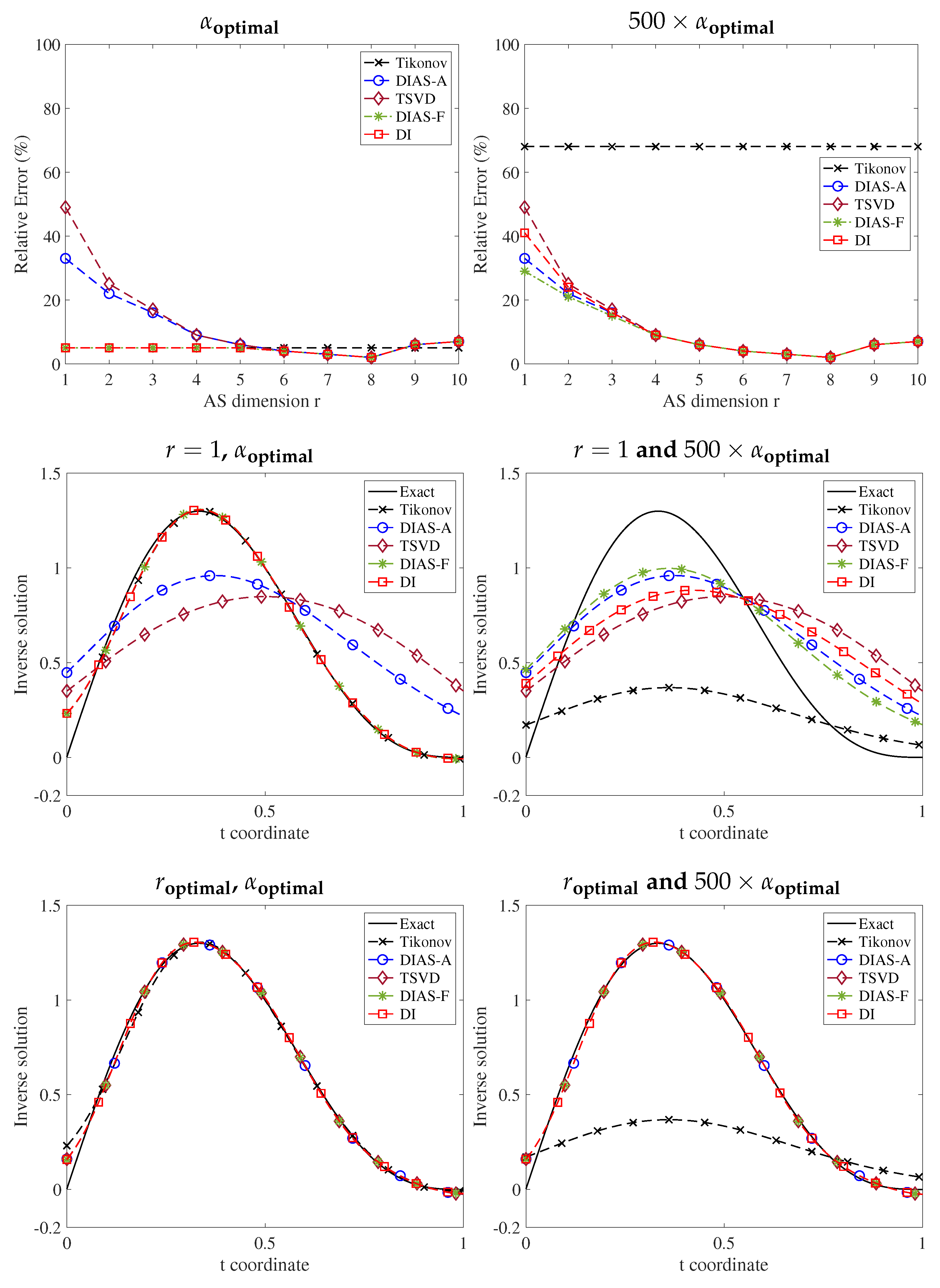
Figure 2 presents solutions for the 1D deconvolution problem with various combinations of active subspace dimension r and regularization parameter . For the one-dimensional active subspace , the TSVD method is not able to reconstruct the solution since the first mode of contributes very little to the true solution. On the contrary, DIAS-A yields a reasonable solution, as its first mode is the most data-informative one. For large dimensional active subspace, the DIAS-A and TSVD solutions are almost the same. These observations are consistent with the discussion following Lemma 1. Recall that the uncentered eigenvectors are a reordering and rotation of the centered ones. By considering a sufficiently large number of modes to be data informed, the subspaces spanned by and become more similar. This can also be clearly seen in Table 2 along the diagonal. Notice that except for the first two modes. This is because the first two eigenvectors are swapped and slightly rotated. Furthermore, inherited from the DI approach [21], DIAS-A, and TSVD (in fact cDIAS-A) solutions are almost invariant with respect to the regularization parameter. This is not surprising since the DIAS approach, by design, regularizes only the data-uninformed modes. Its solution should remain unaffected if sufficient data-informed modes are taken into account.
Figure 2 also shows that the DIAS-F, DI, and Tikhonov solutions are indistinguishable for small regularization parameter regardless of whether or . This is due to two reasons: (1) the DIAS approaches and Tikhonov regularize inactive modes in the same way, and (2) Tikhonov regularization has little effect on the active modes when the regularization parameter is small, thus having little impact on the inverse solution. The situation changes for larger regularization parameters, especially for . Both DIAS-F and DI, by leaving the active parameters untouched, are insensitive to the regularization while Tikhonov oversmooths the solution by heavily regularizing the active parameters.
Another important observation that Figure 2 conveys is the difference among DIAS approaches with centered and uncentered active subspaces. For , the uncentered approaches DIAS-A and DIAS-F outperform the centered counterparts TSVD and DI, especially for large regularization parameters. In other words, uncentered approaches are more robust to the regularization parameter. The reason is that uncentered methods do not penalize the data-informed direction while the centered ones—without taking data into account—regularize , the most data-informative direction in the basis . As discussed in Section 2, for sufficiently large active subspace dimension , all the DIAS solutions are similar since all methods end up spanning the same subspace. However, at the optimal regularization parameter , determined by the L-curve method [38], the DIAS-F solution is visibly closer to the ground truth than TSVD and Tikhonov.
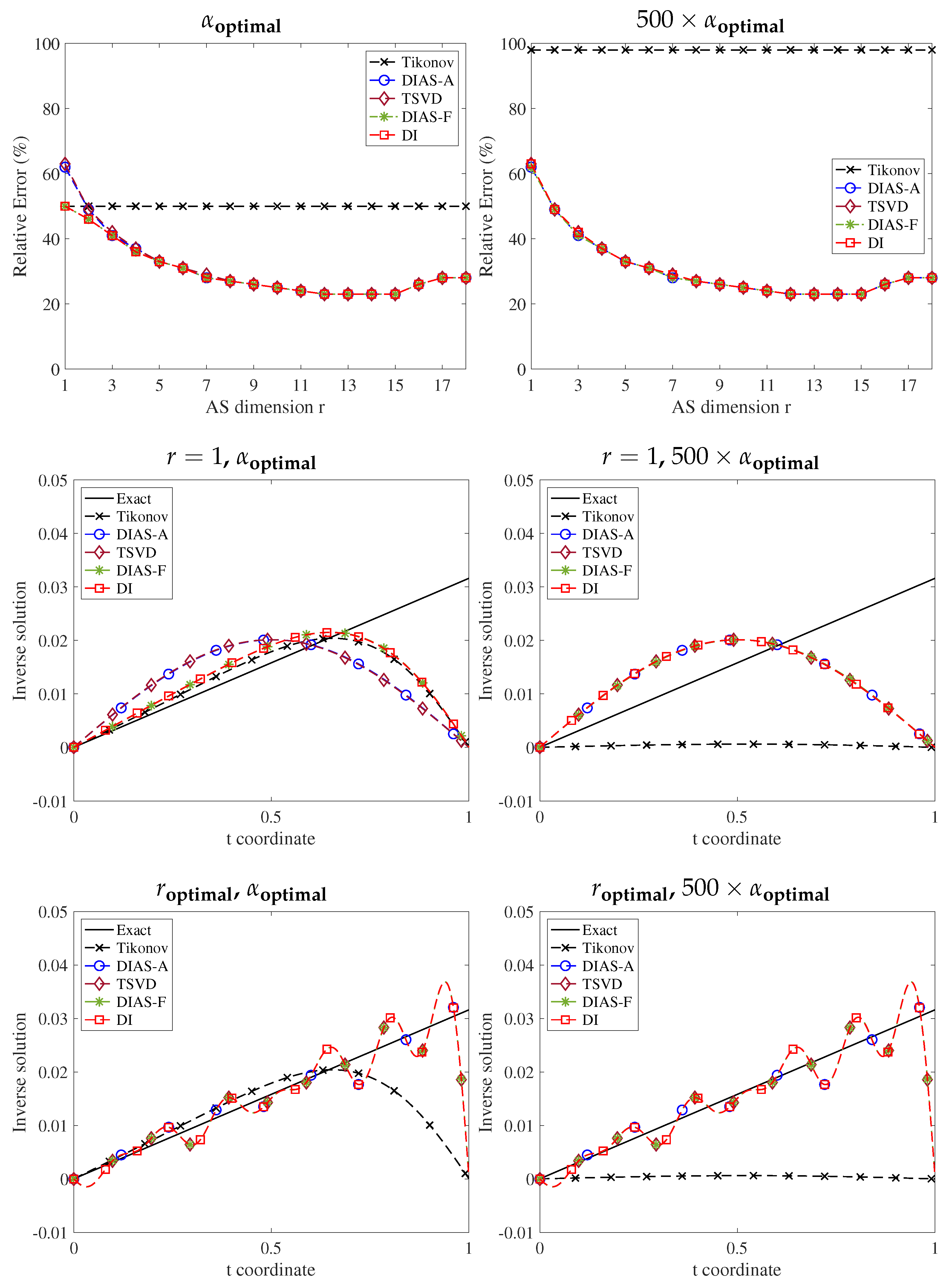
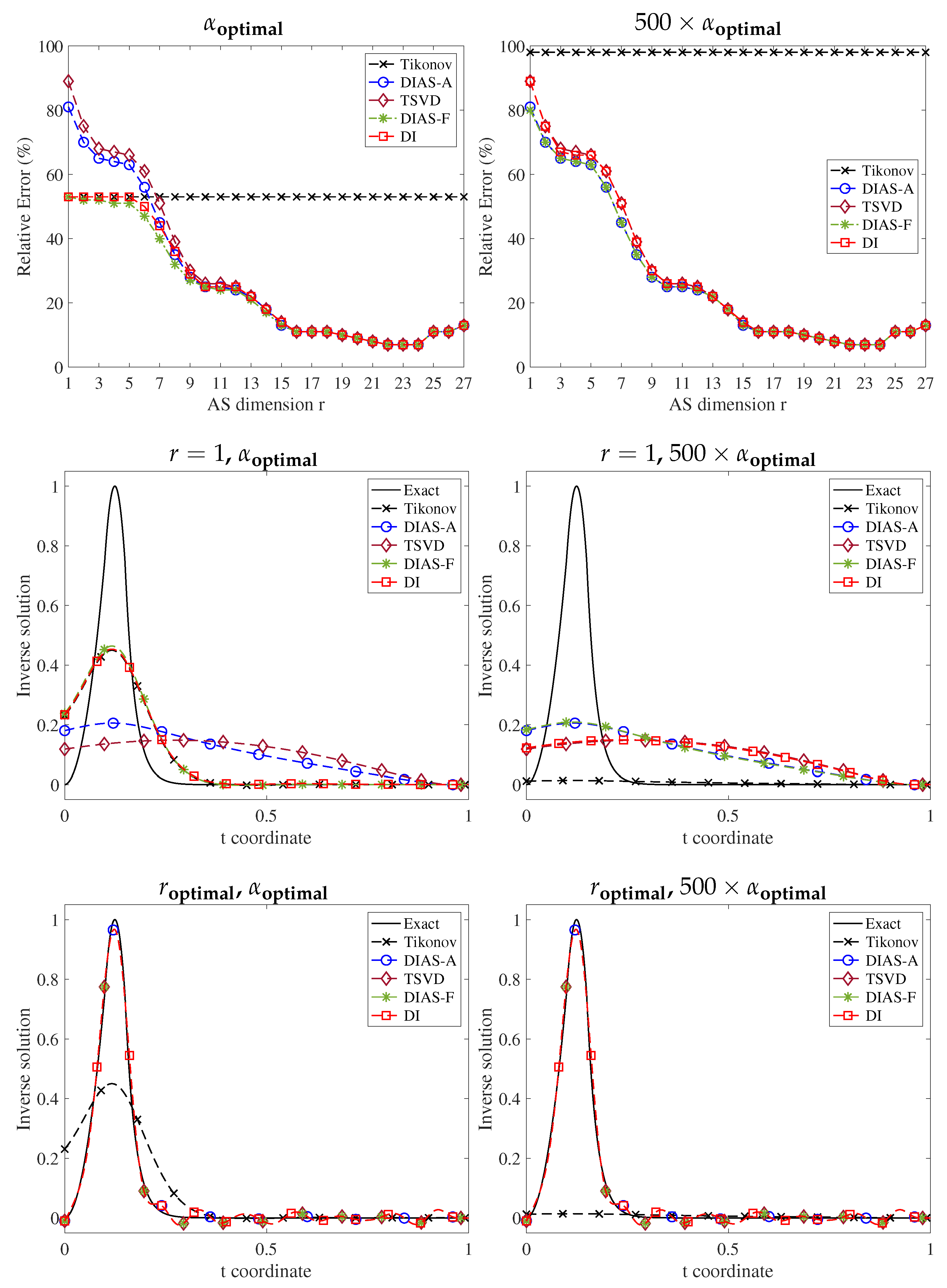
5.2. Benchmark Problems
In this section, we apply the DIAS regularization approach with centered AS and uncentered AS methods to six benchmark problems from regularization tools [38]. We briefly describe the Shaw benchmark [40] here, and we refer the readers to [38] for the descriptions of other benchmark problems. It is in fact a deconvolution problem in which the kernel is given as
where , and the true solution is given by
where . For all benchmark problems, the domain is divided into 1000 subdomains. These problems provide good examples to study the robustness and accuracy properties of the DIAS approaches. Observational data for each problem are corrupted with 1% additive white noise. Figure 3 measures the relative error between the ground truth and its projection on both centered and uncentered active subspaces with various values of the active subspace dimension r. For Shaw, heat, gravity, and Phillips problems, projecting the exact solution on the uncentered AS results in a lower error than on the centered AS. For the Deriv2 and Foxgood problems, the results are identical for both centered and uncentered AS. The reason is that the data for these two problems do not provide new information and thus the active subspaces are entirely determined by the forward operator .
Figure 4, Figure 5, Figure 6, Figure 7, Figure 8 and Figure 9 show the following: (1) top row—relative errors in the inverse solutions for different regularization methods for two values of regularization parameter ( and ); (2) middle row—inverse solutions with Tikhonov regularization and DIAS regularizations with one dimensional active subspace () for two values of regularization parameter; and (3) bottom row—inverse solutions with Tikhonov regularization and DIAS regularizations with optimal active subspace dimension for two values of the regularization parameter. Here, the optimal regularization parameters are chosen based on the L-curve method with Tikhonov regularization [38], and the optimal AS dimension is found experimentally for each method. It turns out that the optimal AS dimension is the same for all methods.
Around the optimal AS dimension (top rows of all figures), regardless of what the regularization parameter is, all DIAS regularizations have similar accuracy and they are more accurate than Tikhonov, as expected. As can be seen in the middle rows, when the active subspace dimension is from to , less than the optimal dimension for the Shaw problem, the full data misfit methods outperform the approximated misfit counterparts. We provide the reason only for the Shaw problem, as it is the same for others. When taking , the approximate misfit approaches completely remove six other active modes, which are misclassified as inactive, in addition to removing the truly inactive modes. The inverse solutions thus lack the important contribution from these modes, leading to inaccurate reconstructions. Even when the active subspace is chosen to be too small, the full misfit methods only regularize the misclassified modes rather than eliminating them from the solution entirely.
The results also show that the DIAS regularizations with full data misfit are at least as good as Tikhonov regularization with and are more accurate with . Again, the reason is that for a reasonably small regularization parameter, the smoothing effect from Tikhonov regularization does not change the solution significantly. On the bottom rows where the AS dimensions are optimal, DIAS solutions are similar and outperform the Tikhonov counterparts for both values of regularization parameters.
From middle to bottom rows, the DIAS solutions with approximate data misfit change from worse to comparable to the DIAS solutions with original data misfit, and thus from worse to more accurate than Tikhonov solutions. This is not surprising: Equation (2) shows that as the active subspace dimension increases, the error due to the data misfit approximation decreases. On the other hand, for the same reasons as in the deconvolution problem, the uncentered AS methods (DIAS-A and DIAS-F) are more accurate than the corresponding centered AS counterparts (TSVD and DI) for all problems with any active subspace dimension and with any regularization parameter.
Note that for these benchmarks, we take as a large regularization parameter case to show that DIAS regularization is robust with respect to the choice of regularization parameter while Tikhonov is not. The DIAS solutions are much more accurate than the Tikhonov solutions, as the latter overregularizes all modes in this case. Additionally, we observe that the full data misfit approaches become similar to the approximate misfit ones as the regularization parameter increases. To see why, we recall from Equation (7) that the only difference between approximate and full misfit approaches is the removal of the inactive variables in the former. When the regularization parameter approaches infinity, it annihilates the contribution of the inactive subspace in the inverse solution. In fact, they behave like TSVD in the limit and we know that TSVD is equivalent to applying infinite regularization on the truncated modes [21]. Thus both approaches would yield identical solutions in the limit. For the case we consider here, the regularization is sufficiently large for us to already see this asymptotic behavior.
5.3. X-ray Tomography
X-ray tomographic reconstruction is another well-known linear inverse problem. A more detailed description of this problem can be found in [9]. Synthetic data are generated with 1%, 3% and 5% white noise added to be realistic. Tikhonov solutions using the optimal regularization parameter , obtained by the L-curve method [9], are compared with DIAS approaches.
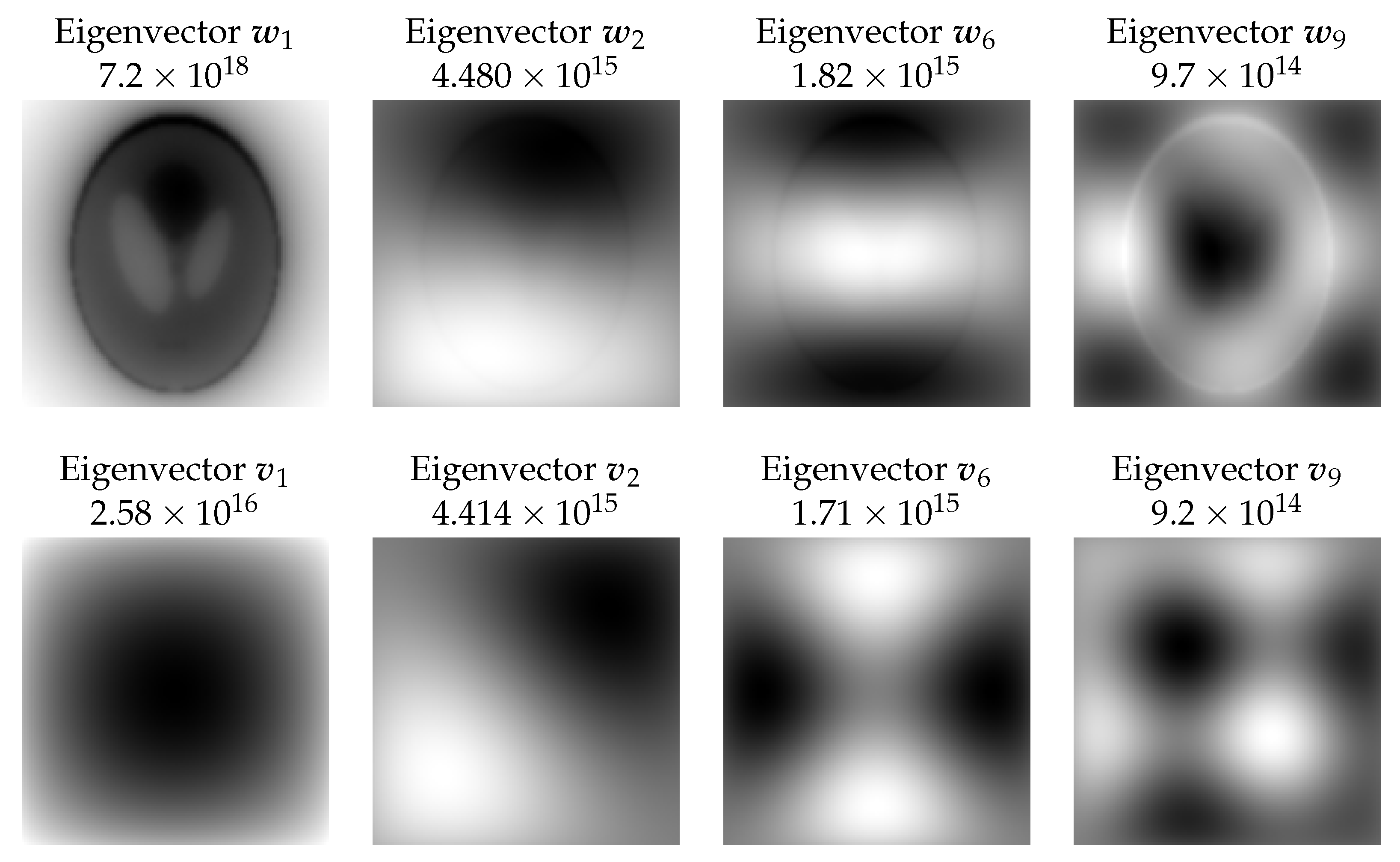
Figure 10 depicts the eigenvalues of and . While the first eigenvalue of the uncentered active subspace matrix is significantly larger than the first eigenvalue of the centered active subspace matrix, this only hints that is more important than any of the vectors in . Figure 11 shows that there is indeed a striking difference between the first eigenvector of the two active subspaces. Visual inspection of the eigenvectors and makes it obvious that contributes significantly to the solution, while the contribution of to the solution is much less pronounced.
The Tikhonov solutions with different regularization parameters and the original image are shown in the Figure 12 for the case of noise. Clearly, underregularization results in noisy solutions and overregularization yields overly smoothed and blurry solutions.
Table 3 and Figure 13 show the relative error and the reconstructed images for the underregularization case. The approximated misfit methods (DIAS-A and TSVD) remove the inactive variables so they are not prone to noise pollution amplified by inverting the small singular values corresponding to these data-uninformed modes. This has a regularization effect known as regularization by truncation. Since the full misfit approaches and Tikhonov capture all modes, their solutions are much more vulnerable to noise in the underregularization regime. For optimal regularization case in Table 4 and Figure 14, the full misfit methods DIAS-F and DI are more accurate than their approximate misfit counterparts for small active subspace dimensions, while all methods give similar results when the active subspace dimension is sufficiently large. For the overregularization case in Table 5 and Figure 15, the approximate and full misfit approaches provide comparable solutions, as they both behave like the TSVD method. Moreover, DIAS regularization solutions are robust to the regularization parameter as opposed to the Tikhonov solution. Another observation is that DIAS methods perform poorly when the active subspace dimension is taken to be too large ( 12,000). This is not surprising since as , all regularization is removed and the problem becomes ill-posed again.
To better understand the robustness of the DIAS approaches to various noise levels, we perform a sensitivity analysis, increasing the noise levels to 3% and 5%. One might expect that the DIAS method would be especially sensitive to noise since it is a data-driven approach. The following discussion shows, however, that the DIAS approaches maintain their advantages, even in the presence of significant noise. The results with higher noise levels are presented in Table 6, Table 7 and Table 8 for 3%, and Table 9, Table 10 and Table 11 for 5%. It can be observed that approximately the first 500 modes of the active subspace are not perturbed by noise (1%, 3% and 5%). For example, at , the relative error of DIAS-A and TSVD are approximately 49% and 56%, respectively, for all noise levels. Meanwhile, when , the corresponding figures for both approaches in the cases of 1%, 3% and 5% are (27.39%, 29.10%), (33.95%, 35.10%) and (43.49 % and 44.39%), respectively. This is consistent with the well-known fact that higher modes of the active subspace (corresponding to smaller eigenvalues) contain more noise. In other words, as the noise level increases, the 5000-th mode moves to the inactive side of the space because it becomes dominated by noise rather than useful information.
6. Conclusions
We have presented four different data-informed regularization approaches for linear inverse problems using active subspaces (DIAS): two with approximate data misfit, and two with full data misfit. We rigorously showed the connection between the centered and uncentered active subspaces and the consequences on the performance of the corresponding DIAS approaches. For linear inverse problems, we showed that the TSVD and the DI regularization methods are members of DIAS regularization. Regularizing only the inactive directions is fundamental to the success of the DIAS approaches. All four DIAS regularization methods are robust to a wide range of regularization parameter values and outperform Tikhonov regularization for many choices of regularization parameter. The uncentered DIAS approaches are more robust and more accurate than their centered counterparts (the TSVD and DI approaches). Among DIAS regularizations methods, DIAS-F (uncentered active subspace with the original data misfit) has the best compromise: it is a data-informed non-intrusive approach.
By data-informed, we mean that the method balances the information encoded in the forward operator and information gained from the particular realization of the data. By non-intrusive, we mean that the method provides the ability to reuse existing inverse codes with minor modification only on the regularization. Various numerical results have demonstrated that the DIAS-F approach is the most effective method presented. In particular, excellent results can be obtained from DIAS-F with only a one-dimensional data informed subspace.
For problems with significant noise in the data, DIAS regularization methods could result in noisy reconstructions unless a small number of active directions are taken, since the less data-informed directions, reflecting the noise in the data, still need some regularization to smooth out the noise. Ongoing work is to equip the DIAS regularization approach with a mechanism to combat high noise scenarios while ensuring the fidelity of inverse solutions. Another appealing feature of the DIAS framework is that it is applicable not only for linear, but also seamlessly for nonlinear inverse problems. Detailed numerical investigations and rigorous analysis of the DIAS approach for nonlinear inverse problems are part of ongoing work.
Author Contributions
Conceptualization, H.N., J.W. and T.B.-T.; Methodology, H.N., J.W. and T.B.-T.; Project administration, H.N., J.W. and T.B.-T.; Supervision, T.B.-T.; Validation, H.N., J.W. and T.B.-T.; Writing—original draft, H.N., J.W. and T.B.-T.; Writing—review and editing, H.N., J.W. and T.B.-T. All authors have read and agreed to the published version of the manuscript.
Funding
This work was partially funded by the National Science Foundation awards NSF-2108320, NSF-1808576 and NSF-CAREER-1845799; by the Department of Energy award DE-SC0018147 and DE-26083989; and by 2020 ConTex award; and by 2021 UT-Portugal CoLab award.
Institutional Review Board Statement
Not applicable.
Informed Consent Statement
Not applicable.
Data Availability Statement
Data are contained within the article.
Acknowledgments
The authors would like to thank the anonymous reviewers for their critical and thoughtful comments that helped improve the paper substantially.
Conflicts of Interest
The authors declare no conflict of interest.
Appendix A. Dias Regularization with Whitened Active Subspaces
One can alternatively whiten the inverse problem to reduce to the standard form. Let us define the following whitening transformation: , , , and .
The whitened inverse problem reads
The corresponding misfit function and its gradient are given as
By simple algebraic manipulations, we obtain
We only consider the DIAS regularization with full misfit (similar derivation can be done for approximate misfit). The uncentered and centered DIAS solutions in this case are
The 1D deconvolution DIAS inverse solutions with non-identity regularization, inspired by the relax boundary prior covariance in [41], show that the whitened active subspace is less accurate (Figure A1).
Figure A1.
The relative error of original active subspace and whitened active subspace in the overregularization case.
Figure A1.
The relative error of original active subspace and whitened active subspace in the overregularization case.

References
- Natterer, F. The Mathematics of Computerized Tomography; SIAM: Philadelphia, PA, USA, 2001. [Google Scholar]
- Natterer, F.; Wübbeling, F. Mathematical Methods in Image Reconstruction; SIAM: Philadelphia, PA, USA, 2001. [Google Scholar]
- Kravaris, C.; Seinfeld, J.H. Identification of parameters in distributed parameter systems by regularization. SIAM J. Control. Optim. 1985, 23, 217–241. [Google Scholar] [CrossRef] [Green Version]
- Banks, H.T.; Kunisch, K. Estimation Techniques for Distributed Parameter Systems; Springer: Berlin/Heidelberg, Germany, 2012. [Google Scholar]
- Bui-Thanh, T.; Ghattas, O.; Martin, J.; Stadler, G. A computational framework for infinite-dimensional Bayesian inverse problems Part I: The linearized case, with application to global seismic inversion. SIAM J. Sci. Comput. 2013, 35, A2494–A2523. [Google Scholar] [CrossRef] [Green Version]
- Bui-Thanh, T.; Burstedde, C.; Ghattas, O.; Martin, J.; Stadler, G.; Wilcox, L.C. Extreme-scale UQ for Bayesian inverse problems governed by PDEs. In Proceedings of the SC’12: International Conference on High Performance Computing, Networking, Storage and Analysis, Salt Lake City, UT, USA, 10–16 November 2012; pp. 1–11. [Google Scholar]
- Colton, D.; Kress, R. Inverse Acoustic and Electromagnetic Scattering, 2nd ed.; Applied Mathematical Sciences; Springer: Berlin/Heidelberg, Germany; New York, NY, USA; Tokyo, Japan, 1998; Volume 93. [Google Scholar]
- Hansen, P.C. Discrete Inverse Problems: Insight and Algorithms; SIAM: Philadelphia, PA, USA, 2010. [Google Scholar]
- Mueller, J.L.; Siltanen, S. Linear and Nonlinear Inverse Problems with Practical Applications; Society for Industrial and Applied Mathematics: Philadelphia, PA, USA, 2012. [Google Scholar]
- Rudin, L.; Osher, S.; Fatemi, E. Nonlinear total variation based noise removal algorithms. Physica D 1992, 60, 259–268. [Google Scholar] [CrossRef]
- Beck, A.; Teboulle, M. Fast Gradient-Based Algorithms for Constrained Total Variation Image Denoising and Deblurring Problems. IEEE Trans. Image Process. 2009, 18, 2419–2434. [Google Scholar] [CrossRef] [Green Version]
- Nikolova, M. Weakly Constrained Minimization: Application to the Estimation of Images and Signals Involving Constant Regions. J. Math. Imaging Vis. 2004, 21, 155–175. [Google Scholar] [CrossRef]
- Goldstein, T.; Osher, S. The slit Bregman method for L1-regularized problems. SIAM J. Imaging Sci. 2009, 2, 323–343. [Google Scholar] [CrossRef]
- Ramirez-Giraldo, J.; Trzasko, J.; Leng, S.; Yu, L.; Manduca, A.; McCollough, C.H. Nonconvex prior image constrained compressed sensing (NCPICCS): Theory and simulations on perfusion CT. Med. Phys. 2011, 38, 2157–2167. [Google Scholar] [CrossRef] [Green Version]
- Babacan, S.D.; Mancera, L.; Molina, R.; Katsaggelos, A.K. Non-convex priors in Bayesian compressed sensing. In Proceedings of the 2009 17th European Signal Processing Conference, Glasgow, UK, 24–28 August 2009; pp. 110–114. [Google Scholar]
- Nikolova, M. Analysis of the recovery of edges in images and signals by minimizing nonconvex regularized least-squares. Multiscale Model. Simul. 2005, 4, 960–991. [Google Scholar] [CrossRef]
- Chartrand, R.; Wohlberg, B. A Nonconvex ADMM Algorithm for Group Sparsity with Sparse Groups. In Proceedings of the 2013 IEEE International Conference on Acoustics, Speech and Signal Processing, Vancouver, BC, Canada, 26–31 May 2013; pp. 6009–6013. [Google Scholar]
- Boley, D. Local linear convergence of the alternating direction method of multipliers on quadratic or linear programs. SIAM J. Optim. 2013, 23, 2183–2207. [Google Scholar] [CrossRef] [Green Version]
- Boyd, S.; Parikh, N.; Chu, E.; Peleato, B.; Eckstein, J. Distributed Optimization and Statistical Learning via the Alternating Direction Method of Multipliers. Found. Trends Mach. Learn. 2010, 3, 1–122. [Google Scholar] [CrossRef]
- Chartrand, R.; Yin, W. Iteratively reweighted algorithms for compressive sensing. In Proceedings of the 2008 IEEE International Conference on Acoustics, Speech and Signal Processing, Las Vegas, NV, USA, 31 March–4 April 2008; pp. 3869–3872. [Google Scholar]
- Wittmer, J.; Bui-Thanh, T. Data-Informed Regularization for Inverse and Imaging Problems. In Handbook of Mathematical Models and Algorithms in Computer Vision and Imaging; Springer International Publishing: Cham, Switzerland, 2021. [Google Scholar]
- Constantine, P.G.; Dow, E.; Wang, Q. Active subspace methods in theory and practice: Applications to kriging surfaces. SIAM J. Sci. Comput. 2014, 36, A1500–A1524. [Google Scholar] [CrossRef]
- Constantine, P.G.; Emory, M.; Larsson, J.; Iaccarino, G. Exploiting active subspaces to quantify uncertainty in the numerical simulation of the HyShot II scramjet. J. Comput. Phys. 2015, 302, 1–20. [Google Scholar] [CrossRef] [Green Version]
- Diaz, P.; Constantine, P.; Kalmbach, K.; Jones, E.; Pankavich, S. A modified SEIR model for the spread of Ebola in Western Africa and metrics for resource allocation. Appl. Math. Comput. 2018, 324, 141–155. [Google Scholar] [CrossRef] [Green Version]
- Constantine, P.G.; Zaharatos, B.; Campanelli, M. Discovering an active subspace in a single-diode solar cell model. Stat. Anal. Data Mining Asa Data Sci. J. 2015, 8, 264–273. [Google Scholar] [CrossRef] [Green Version]
- Cui, C.; Zhang, K.; Daulbaev, T.; Gusak, J.; Oseledets, I.; Zhang, Z. Active subspace of neural networks: Structural analysis and universal attacks. SIAM J. Math. Data Sci. 2020, 2, 1096–1122. [Google Scholar] [CrossRef]
- Lam, R.R.; Zahm, O.; Marzouk, Y.M.; Willcox, K.E. Multifidelity dimension reduction via active subspaces. SIAM J. Sci. Comput. 2020, 42, A929–A956. [Google Scholar] [CrossRef] [Green Version]
- Constantine, P.G.; Kent, C.; Bui-Thanh, T. Accelerating Markov chain Monte Carlo with active subspaces. SIAM J. Sci. Comput. 2016, 38, A2779–A2805. [Google Scholar] [CrossRef] [Green Version]
- Demo, N.; Tezzele, M.; Rozza, G. A non-intrusive approach for the reconstruction of POD modal coefficients through active subspaces. Comptes Rendus Mécanique 2019, 347, 873–881. [Google Scholar] [CrossRef]
- O’Leary-Roseberry, T.; Villa, U.; Chen, P.; Ghattas, O. Derivative-informed projected neural networks for high-dimensional parametric maps governed by PDEs. Comput. Methods Appl. Mech. Eng. 2022, 388, 114199. [Google Scholar] [CrossRef]
- Cadima, J.; Jolliffe, I.T. On Relationships between Uncentred and Column-Centred Principal Component Analysis. Pak. J. Stat. 2009, 25, 473–503. [Google Scholar]
- Honeine, P. An eigenanalysis of data centering in machine learning. arXiv 2014, arXiv:1407.2904. [Google Scholar]
- Jolliffe, I.T.; Cadima, J. Principal component analysis: A review and recent developments. Philos. Trans. R. Soc. Math. Phys. Eng. Sci. 2016, 374, 20150202. [Google Scholar] [CrossRef] [PubMed]
- Alexandris, N.; Gupta, S.; Koutsias, N. Remote sensing of burned areas via PCA, Part 1; centering, scaling and EVD vs. SVD. Open Geospat. Data Softw. Stand. 2017, 2, 17. [Google Scholar] [CrossRef] [Green Version]
- Golub, G.H. Some Modified Matrix Eigenvalue Problems. SIAM Rev. 1973, 15, 318–334. [Google Scholar] [CrossRef] [Green Version]
- Wilkinson, J. The Algebraic Eigenvalue Problem; Claredon Press: Oxford, UK, 1965. [Google Scholar]
- Kirsch, A. An Introduction to the Mathematical Theory of Inverse Problems, 2nd ed.; Applied Mathematical Sciences; Springer: New York, NY, USA, 2011; Volume 120. [Google Scholar]
- Hansen, P.C. Regularization tools version 4.0 for Matlab 7.3. Numer. Algorithms 2007, 46, 189–194. [Google Scholar] [CrossRef]
- Calvetti, D.; Somersalo, E. An Introduction to Bayesian Scientific Computing: Ten Lectures on Subjective Computing; Springer: Berlin/Heidelberg, Germany, 2007; Volume 2. [Google Scholar]
- Shaw, C., Jr. Improvement of the resolution of an instrument by numerical solution of an integral equation. J. Math. Anal. Appl. 1972, 37, 83–112. [Google Scholar] [CrossRef] [Green Version]
- Calvetti, D. Preconditioned iterative methods for linear discrete ill-posed problems from a Bayesian inversion perspective. J. Comp. Appl. Math. 2007, 2, 378–395. [Google Scholar] [CrossRef] [Green Version]
Figure 1.
1D deconvolution problem. (a): uncentered AS subspace versus centered AS subspace in representing the true solution. (b): relative error of DIAS-A and TSVD solutions as a function of active subspace dimension r.
Figure 1.
1D deconvolution problem. (a): uncentered AS subspace versus centered AS subspace in representing the true solution. (b): relative error of DIAS-A and TSVD solutions as a function of active subspace dimension r.

Figure 2.
Solutions for 1D deconvolution problem with different active subspace dimensions and different regularization parameter values .
Figure 2.
Solutions for 1D deconvolution problem with different active subspace dimensions and different regularization parameter values .

Figure 3.
The comparison between centered AS and uncentered AS in recovering the true solution . is the projection of in the active subspaces.
Figure 3.
The comparison between centered AS and uncentered AS in recovering the true solution . is the projection of in the active subspaces.

Figure 4.
Shaw problem, . Comparison of different DIAS regularizations and Tikhonov regularization. Top row: relative errors in the inverse solutions for different regularization methods for two values of regularization parameter. Middle row: inverse solutions with DIAS regularizations with one-dimensional active subspace and Tikhonov regularization for two values of regularization parameter. Bottom row: inverse solutions with DIAS regularizations with the optimal dimension active subspace () and Tikhonov regularization for two values of regularization parameter.

Figure 5.
Gravity, . Comparison of different DIAS regularizations and Tikhonov regularization. Top row: relative errors in the inverse solutions for different regularization methods for two values of regularization parameter. Middle row: inverse solutions with DIAS regularizations with one-dimensional active subspace and Tikhonov regularization for two values of regularization parameter. Bottom row: inverse solutions with DIAS regularizations with the optimal dimension active subspace () and Tikhonov regularization for two values of regularization parameter.

Figure 6.
Deriv2, . Comparison of different DIAS regularizations and Tikhonov regularization. Top row: relative errors in the inverse solutions for different regularization methods for two values of regularization parameter. Middle row: inverse solutions with DIAS regularizations with one-dimensional active subspace and Tikhonov regularization for two values of regularization parameter. Bottom row: inverse solutions with DIAS regularizations with the optimal dimension active subspace () and Tikhonov regularization for two values of regularization parameter.

Figure 7.
Heat, . Comparison of different DIAS regularizations and Tikhonov regularization. Top row: relative errors in the inverse solutions for different regularization methods for two values of regularization parameter. Middle row: inverse solutions with DIAS regularizations with one-dimensional active subspace and Tikhonov regularization for two values of regularization parameter. Bottom row: inverse solutions with DIAS regularizations with the optimal dimension active subspace () and Tikhonov regularization for two values of regularization parameter.

Figure 8.
Phillips, . Comparison of different DIAS regularizations and Tikhonov regularization. Top row: relative errors in the inverse solutions for different regularization methods for two values of regularization parameter. Middle row: inverse solutions with DIAS regularizations with one-dimensional active subspace and Tikhonov regularization for two values of regularization parameter. Bottom row: inverse solutions with DIAS regularizations with the optimal dimension active subspace () and Tikhonov regularization for two values of regularization parameter.

Figure 9.
Foxgood, . Comparison of different DIAS regularizations and Tikhonov regularization. Top row: relative errors in the inverse solutions for different regularization methods for two values of regularization parameter. Middle row: inverse solutions with DIAS regularizations with one-dimensional active subspace and Tikhonov regularization for two values of regularization parameter. Bottom row: inverse solutions with DIAS regularizations with the optimal dimension active subspace () and Tikhonov regularization for two values of regularization parameter.

Figure 10.
The spectrum of (Uncentered Active Subspace) and (Centered Active Subspace), noise level 1%.
Figure 10.
The spectrum of (Uncentered Active Subspace) and (Centered Active Subspace), noise level 1%.

Figure 11.
Eigenvectors of uncentered AS and centered AS , and their corresponding eigenvalues, noise level 1%.
Figure 11.
Eigenvectors of uncentered AS and centered AS , and their corresponding eigenvalues, noise level 1%.

Figure 12.
Solutions for X-ray tomography using Tikhonov regularization with regularization parameters and the original image (right-most), noise level 1%.
Figure 12.
Solutions for X-ray tomography using Tikhonov regularization with regularization parameters and the original image (right-most), noise level 1%.

Figure 13.
DIAS solutions for X-ray tomography problem with underregularization parameter , noise level 1%.
Figure 13.
DIAS solutions for X-ray tomography problem with underregularization parameter , noise level 1%.

Figure 14.
DIAS solutions for X-ray tomography problem with optimal regularization parameter , noise level 1%.
Figure 14.
DIAS solutions for X-ray tomography problem with optimal regularization parameter , noise level 1%.

Figure 15.
DIAS solutions for X-ray tomography problem with overregularization parameter , noise level 1%.
Figure 15.
DIAS solutions for X-ray tomography problem with overregularization parameter , noise level 1%.


Table 1.
Comparison of features between different approaches (✓ = possess, ✗ = not possess).
| TSVD | Tikhonov | DI [21] | DIAS | |
|---|---|---|---|---|
| Solving ill-posed inverse problem | ✓ | ✓ | ✓ | ✓ |
| Parameter robustness/Avoiding regularizing data-informed modes | ✗ | ✗ | ✓ | ✓ |
| Ordering data-informed modes based on observational data | ✗ | ✗ | ✗ | ✓ |
| Readily aplicable to nonlinear inverse problems | ✗ | ✓ | ✗ | ✓ |
| Taking the uncertain nature of the inverse problem into account | ✗ | ✗ | ✗ | ✓ |
Table 2.
between first ten eigenvectors in and .
| −0.01 | 0.97 | 0 | −0.02 | 0 | 0.22 | 0 | −0.01 | 0 | −0.02 | |
| 1 | 0.01 | 0 | 0 | 0 | 0 | 0 | 0 | 0 | 0 | |
| 0 | 0 | 1 | 0 | 0 | 0 | 0 | 0 | 0 | 0 | |
| 0 | 0.02 | 0 | 1 | 0 | −0.01 | 0 | 0 | 0 | 0 | |
| 0 | 0 | 0 | 0 | 1 | 0 | 0 | 0 | 0 | 0 | |
| 0 | −0.22 | 0 | 0.01 | 0 | 0.97 | 0 | −0.01 | 0 | −0.01 | |
| 0 | 0 | 0 | 0 | 0 | 0 | −1 | 0 | 0 | 0 | |
| 0 | 0.01 | 0 | 0 | 0 | 0.01 | 0 | 1 | 0 | 0 | |
| 0 | 0 | 0 | 0 | 0 | 0 | 0 | 0 | 1 | 0 | |
| 0 | 0.02 | 0 | 0 | 0 | 0.01 | 0 | 0 | 0 | 1 |
Table 3.
Relative error (%) of inverse solutions by DIAS and Tikhonov regularization for underregularization case with , noise level 1%.
Table 3.
Relative error (%) of inverse solutions by DIAS and Tikhonov regularization for underregularization case with , noise level 1%.
| Method | Number of Dimensions of Active Subspace | |||||
|---|---|---|---|---|---|---|
| r = 1 | r = 500 | r = 2000 | r = 5000 | r = 10,000 | r = 12,000 | |
| DIAS-A | 79.47 | 49.31 | 36.13 | 27.39 | 22.74 | 35.36 |
| TSVD | 84.58 | 56.50 | 40.17 | 29.10 | 22.98 | 35.36 |
| DIAS-F | 389.15 | 389.16 | 389.15 | 389.16 | 389.13 | 389.01 |
| DI | 389.15 | 389.16 | 389.15 | 389.17 | 389.13 | 389.01 |
| Tikhonov | 389.15 | |||||
Table 4.
Relative error (%) of inverse solutions by DIAS and Tikhonov regularization for optimal regularization case with , noise level 1%.
Table 4.
Relative error (%) of inverse solutions by DIAS and Tikhonov regularization for optimal regularization case with , noise level 1%.
| Method | Number of Dimensions of Active Subspace | |||||
|---|---|---|---|---|---|---|
| r = 1 | r = 500 | r = 2000 | r = 5000 | r = 10,000 | r = 12,000 | |
| DIAS-A | 79.47 | 49.31 | 36.13 | 27.39 | 22.74 | 35.36 |
| TSVD | 84.58 | 56.50 | 40.17 | 29.10 | 22.98 | 35.36 |
| DIAS-F | 21.35 | 21.22 | 21.08 | 21.05 | 22.17 | 35.39 |
| DI | 21.36 | 21.33 | 21.24 | 21.19 | 22.21 | 35.39 |
| Tikhonov | 21.36 | |||||
Table 5.
Relative error (%) of inverse solutions by DIAS and Tikhonov regularization for overregularization case with , noise level 1%.
Table 5.
Relative error (%) of inverse solutions by DIAS and Tikhonov regularization for overregularization case with , noise level 1%.
| Method | Number of Dimensions of Active Subspace | |||||
|---|---|---|---|---|---|---|
| r = 1 | r = 500 | r = 2000 | r = 5000 | r = 10,000 | r = 12,000 | |
| DIAS-A | 79.47 | 49.31 | 36.13 | 27.39 | 22.74 | 35.36 |
| TSVD | 84.58 | 56.50 | 40.17 | 29.10 | 22.98 | 35.36 |
| DIAS-F | 74.29 | 48.65 | 35.91 | 27.32 | 22.73 | 35.36 |
| DI | 78.08 | 55.6 | 39.89 | 29.01 | 22.97 | 35.36 |
| Tikhonov | 80.77 | |||||
Table 6.
Relative error (%) of inverse solutions by DIAS and Tikhonov regularization for underregularization case with , noise level 3%.
Table 6.
Relative error (%) of inverse solutions by DIAS and Tikhonov regularization for underregularization case with , noise level 3%.
| Method | Number of Dimensions of Active Subspace | |||||
|---|---|---|---|---|---|---|
| r = 1 | r = 500 | r = 2000 | r = 5000 | r = 10,000 | r = 12,000 | |
| DIAS-A | 79.47 | 49.42 | 37.32 | 33.95 | 48.46 | 97.10 |
| TSVD | 84.58 | 56.57 | 41.05 | 35.10 | 48.53 | 97.10 |
| DIAS-F | 371.83 | 371.82 | 371.81 | 371.80 | 371.81 | 372.87 |
| DI | 371.83 | 371.83 | 371.83 | 371.81 | 371.81 | 372.88 |
| Tikhonov | 371.83 | |||||
Table 7.
Relative error (%) of inverse solutions by DIAS and Tikhonov regularization for underregularization case with , noise level 3%.
Table 7.
Relative error (%) of inverse solutions by DIAS and Tikhonov regularization for underregularization case with , noise level 3%.
| Method | Number of Dimensions of Active Subspace | |||||
|---|---|---|---|---|---|---|
| r = 1 | r = 500 | r = 2000 | r = 5000 | r = 10,000 | r = 12,000 | |
| DIAS-A | 79.47 | 49.42 | 37.32 | 33.95 | 48.46 | 97.10 |
| TSVD | 84.58 | 56.57 | 41.05 | 35.10 | 48.53 | 97.10 |
| DIAS-F | 33.99 | 32.24 | 30.89 | 32.77 | 48.42 | 97.10 |
| DI | 34.17 | 33.56 | 32.11 | 33.30 | 48.46 | 97.10 |
| Tikhonov | 34.17 | |||||
Table 8.
Relative error (%) of inverse solutions by DIAS and Tikhonov regularization for underregularization case with , noise level 3%.
Table 8.
Relative error (%) of inverse solutions by DIAS and Tikhonov regularization for underregularization case with , noise level 3%.
| Method | Number of Dimensions of Active Subspace | |||||
|---|---|---|---|---|---|---|
| r = 1 | r = 500 | r = 2000 | r = 5000 | r = 10,000 | r = 12,000 | |
| DIAS-A | 79.47 | 49.42 | 37.32 | 33.95 | 48.46 | 97.10 |
| TSVD | 84.58 | 56.57 | 41.05 | 35.10 | 48.52 | 97.10 |
| DIAS-F | 78.77 | 49.34 | 37.30 | 33.95 | 48.46 | 97.10 |
| DI | 83.68 | 56.47 | 41.02 | 35.09 | 48.52 | 97.10 |
| Tikhonov | 95.19 | |||||
Table 9.
Relative error (%) of inverse solutions by DIAS and Tikhonov regularization for underregularization case with , noise level 5%.
Table 9.
Relative error (%) of inverse solutions by DIAS and Tikhonov regularization for underregularization case with , noise level 5%.
| Method | Number of Dimensions of Active Subspace | |||||
|---|---|---|---|---|---|---|
| r = 1 | r = 500 | r = 2000 | r = 5000 | r = 10,000 | r = 12,000 | |
| DIAS-A | 79.47 | 49.54 | 39.03 | 43.49 | 77.18 | 161.65 |
| TSVD | 84.58 | 56.69 | 42.62 | 44.39 | 77.22 | 161.62 |
| DIAS-F | 326.77 | 326.77 | 326.78 | 326.77 | 326.69 | 332.71 |
| DI | 326.77 | 326.77 | 326.78 | 326.78 | 326.69 | 332.71 |
| Tikhonov | 326.77 | |||||
Table 10.
Relative error (%) of inverse solutions by DIAS and Tikhonov regularization for underregularization case with , noise level 5%.
Table 10.
Relative error (%) of inverse solutions by DIAS and Tikhonov regularization for underregularization case with , noise level 5%.
| Method | Number of Dimensions of Active Subspace | |||||
|---|---|---|---|---|---|---|
| r = 1 | r = 500 | r = 2000 | r = 5000 | r = 10,000 | r = 12,000 | |
| DIAS-A | 79.47 | 49.54 | 39.03 | 43.49 | 77.18 | 161.65 |
| TSVD | 84.58 | 56.69 | 42.62 | 44.39 | 77.22 | 161.62 |
| DIAS-F | 43.55 | 38.73 | 35.93 | 43.08 | 77.19 | 161.65 |
| DI | 44.05 | 41.73 | 38.07 | 43.73 | 77.22 | 161.62 |
| Tikhonov | 44.06 | |||||
Table 11.
Relative error (%) of inverse solutions by DIAS and Tikhonov regularization for underregularization case with , noise level 5%.
Table 11.
Relative error (%) of inverse solutions by DIAS and Tikhonov regularization for underregularization case with , noise level 5%.
| Method | Number of Dimensions of Active Subspace | |||||
|---|---|---|---|---|---|---|
| r = 1 | r = 500 | r = 2000 | r = 5000 | r = 10,000 | r = 12,000 | |
| DIAS-A | 79.47 | 49.54 | 39.03 | 43.49 | 77.18 | 161.65 |
| TSVD | 84.58 | 56.69 | 42.62 | 44.39 | 77.22 | 161.61 |
| DIAS-F | 79.21 | 49.52 | 39.02 | 43.49 | 77.18 | 161.64 |
| DI | 84.25 | 56.66 | 42.61 | 44.38 | 77.22 | 161.61 |
| Tikhonov | 98.06 | |||||
Publisher’s Note: MDPI stays neutral with regard to jurisdictional claims in published maps and institutional affiliations. |
© 2022 by the authors. Licensee MDPI, Basel, Switzerland. This article is an open access article distributed under the terms and conditions of the Creative Commons Attribution (CC BY) license (https://creativecommons.org/licenses/by/4.0/).
Share and Cite
MDPI and ACS Style
Nguyen, H.; Wittmer, J.; Bui-Thanh, T. DIAS: A Data-Informed Active Subspace Regularization Framework for Inverse Problems. Computation 2022, 10, 38. https://0-doi-org.brum.beds.ac.uk/10.3390/computation10030038
AMA Style
Nguyen H, Wittmer J, Bui-Thanh T. DIAS: A Data-Informed Active Subspace Regularization Framework for Inverse Problems. Computation. 2022; 10(3):38. https://0-doi-org.brum.beds.ac.uk/10.3390/computation10030038
Chicago/Turabian StyleNguyen, Hai, Jonathan Wittmer, and Tan Bui-Thanh. 2022. "DIAS: A Data-Informed Active Subspace Regularization Framework for Inverse Problems" Computation 10, no. 3: 38. https://0-doi-org.brum.beds.ac.uk/10.3390/computation10030038
Note that from the first issue of 2016, this journal uses article numbers instead of page numbers. See further details here.