
Nonadiabatic Exchange-Correlation Potential for Strongly Correlated Materials in the Weak and Strong Interaction Limits


Department of Physics, University of Central Florida, Orlando, FL 32816, USA
*
Author to whom correspondence should be addressed.
Computation 2022, 10(5), 77; https://0-doi-org.brum.beds.ac.uk/10.3390/computation10050077
Submission received: 6 April 2022
/
Revised: 12 May 2022
/
Accepted: 14 May 2022
/
Published: 20 May 2022
(This article belongs to the Special Issue Static and Time-Dependent Density-Functional Theories for Strongly Correlated Materials)
Abstract
:In this work, nonadiabatic exchange-correlation (XC) potentials for time-dependent density-functional theory (TDDFT) for strongly correlated materials are derived in the limits of strong and weak correlations. After summarizing some essentials of the available dynamical mean-field theory (DMFT) XC potentials valid for these systems, we present details of the Sham–Schluter equation approach that we use to obtain, in principle, an exact XC potential from a many-body theory solution for the nonequilibrium electron self-energy. We derive the XC potentials for the one-band Hubbard model in the limits of weak and strong on-site Coulomb repulsion. To test the accuracy of the obtained potentials, we compare the TDDFT results obtained with these potentials with the corresponding nonequilibrium DMFT solution for the one-band Hubbard model and find that the agreement between the solutions is rather good. We also discuss possible directions to obtain a universal XC potential that would be appropriate for the case of intermediate interaction strengths, i.e., a nonadiabatic potential that can be used to perform TDDFT analysis of nonequilibrium phenomena, such as transport and other ultrafast properties of materials with any strength of electron correlation at any value in the applied perturbing field.
1. Introduction
Description of the physical properties of strongly correlated materials, i.e., systems with partially filled, localized d and f electron orbitals, is one of the greatest challenges of modern condensed matter physics and material science. A strong competition between the role of the usually itinerant s- and/or p-states, and the much more localized d- and/or f-states, in these systems produces many new effects that already have applications in technologies. The properties can be further tuned by changing pressure, temperature, the size and composition of the system and other parameters [1,2,3,4]. The nonequilibrium properties of these materials are of a special interest since they can be used in modern technologies that are pushing the limits of “small and fast”. In particular, the ultrafast properties of strongly correlated materials can be used in smart window applications [5], biosensors [6] and switches [7]. It is thus imperative that reliable and accurate strategies be developed for both understanding and predicting the equilibrium and nonequilibrium properties of strongly correlated materials. This task is, however, challenging because of complex processes in these systems driven by both kinetic and potential energy (local electron repulsion) effects: technically, one cannot use a perturbation expansion in either of the corresponding (kinetic or potential energy) terms of the Hamiltonian, and rather, nontrivial, nonperturbative methods have to be applied.
There are also technical difficulties in applying the available nonperturbative many-body tools, such as equilibrium [8] and nonequilibrium [9,10] dynamical mean-field theory (DMFT), to real materials since they typically contain a good number of nonequivalent atoms and require the inclusion of several orbitals in the calculations and/or necessity to use many-argument (complex-time) Green’s functions (GFs) [10]. In this sense, both the static [11,12] and time-dependent [13,14] DFT approaches are much more promising. Indeed, the standard DFT (static) is a theory of one function—the space-dependent charge density. However, DFT exchange–correlation (XC) potentials cannot correctly capture the salient effects of strong electron–electron correlations [15] in materials of interest. The standard LDA, GGA and other DFT functionals usually fail to accurately describe the band gap and even ground state properties of strongly correlated materials, e.g., ground-state properties of antiferromagnetic oxides and orbitally ordered systems [16] (it must be noted that recently it was demonstrated that the DFT potential developed within the adiabatic connection model [17,18] can produce physically meaningful results in strongly correlated cases [19]).
A DFT XC potential can be derived by using a many-body approach, e.g., by calculating the dependencies of the XC energy on the electron charge density n and differentiating this function with respect to . Some progress in this direction has been made in the case of constrained systems (i.e., those that can be solved exactly). The examples include the 0D and 1D systems [20,21,22,23,24,25,26] solved with the Bethe ansatz approach [27] and small clusters [15,28,29,30,31] and 1D systems [28,30,32,33,34] solved exactly numerically with an appropriate tool. The problem of dimensional crossover and possible approaches to constructing corresponding DFT XC functionals and potentials for strongly correlated systems in low dimensions were also discussed in works [35,36,37,38]. On the other hand, to obtain the “universal” XC potential for strongly correlated materials that works in all dimensions, one also needs to know its structure in higher dimensions, i.e., in much more complex 2D and 3D cases. It seems an analytical result for the XC potential for these systems can be obtained only at low electron densities for which a formula for the XC energy as function of density is available [39,40,41]. Several numerical static DFT approaches for strongly correlated systems also exist, such as the Gutzwiller DFT [42,43] (with the energy functional obtained from the projected Gutzwiller wave functions), the one-body reduced density-matrix functional theory [44], the lattice DFT [45], the strictly-correlated-electrons DFT [18,46] and the DMFT-DFT with XC potential built from the results for the XC energy for the 3D one-band Hubbard model [47] and for the infinite-dimensional Holstein–Hubbard model [48]. The last approach is probably the most promising since DMFT is capable of covering all regimes in correlated systems (from weak to strong correlations). Recently, a novel machine-learning methodology based on exact-diagonalization results was used to build an exact XC functional for the Hubbard model [49]. For a review of some other functionals obtained with different approximations, we refer the reader to Ref. [15].
In the time-dependent case, TDDFT is an even more advantageous approach for application to strongly correlated materials as compared to the many-body methods since there are fewer (one) time arguments in the equations. For the “usual” (weakly correlated) materials, DFT was used to analyze systems with hundreds of atoms [50,51]. To apply the tool to strongly correlated materials, one needs, similar to DFT, a relevant XC potential. Some efforts in this direction have also been made [20,21,22,33,47,52,53,54,55]. In the derivation of the TDDFT XC potentials for strongly correlated systems, exactly solvable models for low dimensional systems, such as chains [20,21,22,33,55], Bethe-ansatz [27] solution or small-cluster [15,28,29,30,31,54,56,57,58] (exact diagonalization) methods have been applied. The standard strategy in the above was to calculate the dependence of the static XC energy in the Hubbard model on the electron density, , to differentiate the result with respect to the density to obtain the static XC potential, , and to substitute in the last dependence to obtain the TDDFT adiabatic XC potential . The resulting potentials allowed one to describe Mott insulator transitions (MIT) and some other nonequilibrium phenomena. However, it was found that the results obtained with the adiabatic potential, for example, for the response of the 1D Hubbard model, became inaccurate or even wrong as U increased or the doping approached half-filling (i.e., when the system approaches the regime of strong correlations) [33]. One of the reasons for this could be lack of nonadiabatic effects, i.e., missing memory in the XC potential (in the case of GGA potentials, the reason could also be a large reduced gradient in the strongly correlated cases (of localized charges), which leads to noncorrect predictions [38]).
The situation is similar in higher dimensions. In particular, Karlsson et al. [47] obtained with DMFT the static dependence and the TDDFT adiabatic XC potential for the 3D one-band Hubbard model. Similar to the 1D case, it was found that the obtained XC potential does not work well when U is large and/or when the system is close to half-filling, once more suggesting importance of nonadiabatic effects (for the importance of these effects in the cases of Hubbard dimer and Hubbard chains, see, e.g., Refs. [56,57,59] and [60], respectively). Recently, the linear-response TDDFT nonadiabatic XC potential (XC kernel) was calculated with DMFT for both spin-independent (infinite-dimensional Hubbard model) [61] and spin-dependent (noncollinear) (bulk Ni) [62] cases. In these works, the kernels were derived from the DMFT charge and spin susceptibilities, respectively (it must be mentioned that almost two decades ago, nonadiabatic XC kernels for Hubbard clusters were also obtained from charge susceptibility [54]).
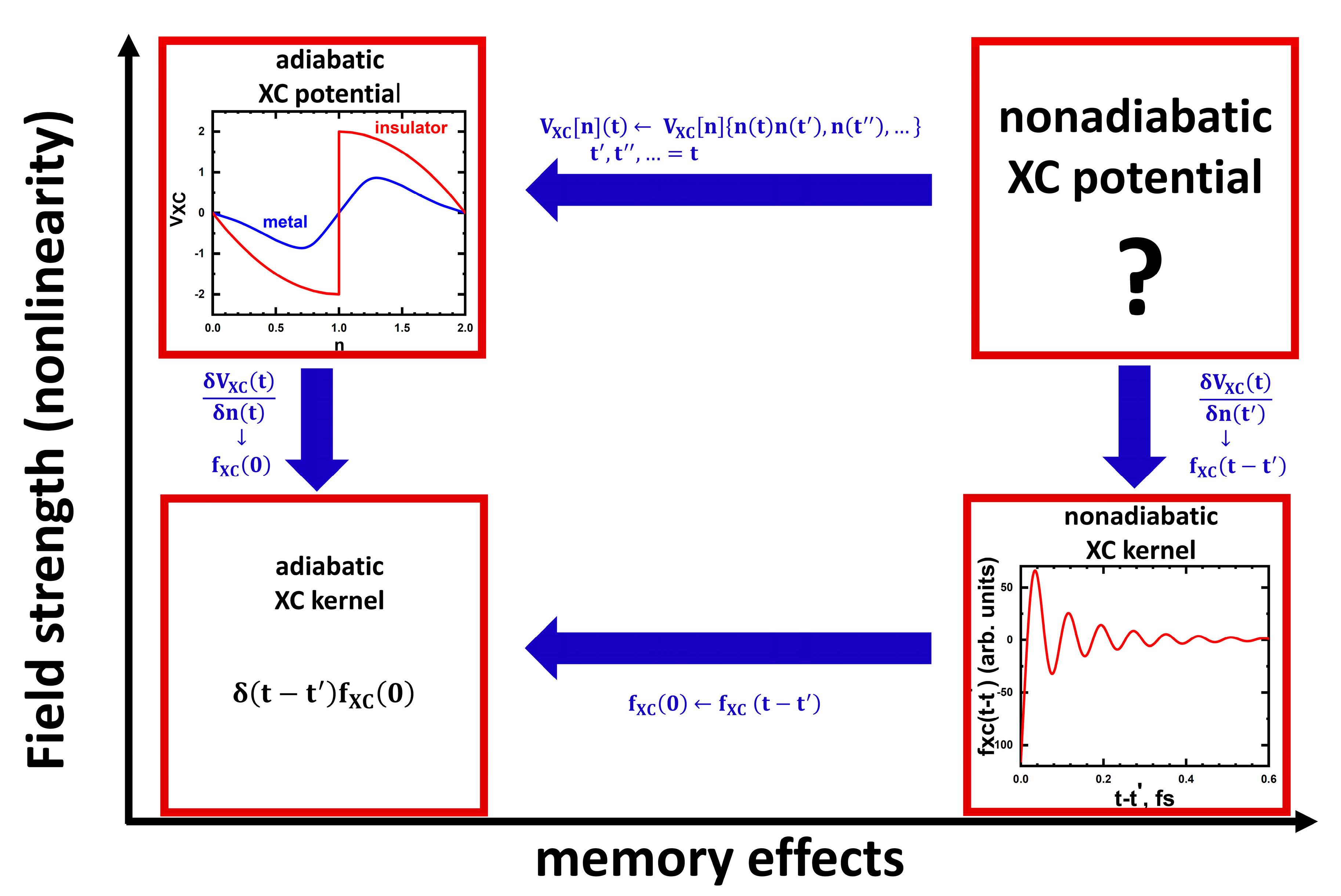
To summarize, for “large” (bulk) systems, currently we have available nonlinear adiabatic (one-band Hubbard model) and linear nonadiabatic (many-band Hubbard model) DMFT XC potentials (more accurately, in the last case, tools to calculate them), but the problem of finding general TDDFT nonlinear nonadiabatic XC potentials for multi-band systems still needs to be solved (the situation is schematically shown in Figure 1, in which the connections between different approximations for the XC potentials are also shown).
In this work, we derive nonadiabatic XC potentials by solving the Hubbard model exactly in the limits of weak and strong correlations when the system is perturbed by an external pulse. The derivation is based on an alternative tool—the Sham–Schluter equation approach [63,64], where is obtained from the many-body theory results for the electron self-energy . We approximate the obtained self-energies by the local-in-space site-independent functions, , relevant to DMFT. In the many-body case, such an approach with nonequilibrium perturbative self-energy was successfully applied to study, e.g., the nonequilibrium current [65]. The obtained potential allows one to accurately take into account the correlation and memory effects in the cases of small and large Us. Additionally, the results can be regarded as a step towards the final goal of deriving the DMFT nonadiabatic XC potential for strongly correlated materials.
The rest of the text is organized as follows. In Section 2, we mention key facts about TDDFT and summarize the previous main results for the DMFT XC potential for the linear-response case for spin-nonpolarized and spin-polarized systems (Section 2.1 and Section 2.2, correspondingly). In Section 3, we summarize the previous results for the nonlinear adiabatic XC potential obtained with DMFT. Details of the Sham–Schluter equation formalism are given in Section 4. In Section 5 and Section 6, we present our results for the XC potentials obtained at small and large values of the local Coulomb repulsion U by solving the Sham–Schluter equation. We conclude, with a summary and a discussion of possible future directions in the field, in Section 7.
2. Linear Response: DMFT Nonadiabatic XC Kernels
To analyze the dynamics of a system with TDDFT, one needs to solve the time-dependent Kohn–Sham (KS) equation [13,14]:
where are quantum numbers, except spin , and
is the KS potential, a unique functional of density that consists of the Hartree , the XC and the external (ions, external fields, etc.) parts. Since one or more parts of the KS potential in Equation (1) depend on the charge density, this equation has to be solved self-consistently with the charge density equation:
In the linear-response regime, the equations are simplified since the dependence of the XC potential on the change density (basically, the only unknown time-dependent quantity in the problem) is rather simple:
where
is the XC kernel. This quantity can be found from the TDDFT equation for the charge susceptibility:
i.e.,
(in frequency representation), provided the susceptibility is known. The remaining undefined function in Equation (7) is KS susceptibility:
where and are the KS eigenenergies (band spectrum) and eigenfunctions, and are the Fermi factors.
In the case of solids, i.e., “infinite” periodic systems, it is more convenient to solve Equation (6) or (7) in the frequency–momentum representation. Namely, in the frequency representation one gets from Equation (6):
Due to periodicity of the response function in real space,
( is the lattice vector), one can use the Fourier transforms for all functions of type
where are reciprocal vectors (and similar for other functions). Then, Equations (6) and (7) in the frequency–momentum space can be written as:
where
is the Fourier transform of the Coulomb potential, and
are the matrix elements of the KS susceptibility.
Provided the XC kernel is known, one can study the dynamics of the system by using Equations (1) and (3) and to analyze other physical properties of the system, such as the absorption spectrum, by using results for the TDDFT susceptibility in Equation (12) (see, e.g., [14]). Below, we discuss solutions of the opposite problem: finding the XC kernel from the results for susceptibility.
2.1. Nonadiabatic DMFT XC Kernel: Paramagnetic Case
In this subsection, we show how to derive the nonadiabatic XC kernel from the Hubbard model susceptibility obtained in the DMFT approximation in the paramagnetic case [61]. For this, we begin by writing down the multi-orbital Hubbard Hamiltonian in standard notation:
where are the inter-site, inter-orbital hopping parameters, is the chemical potential, is the exchange energy parameter and are the site- and orbital-dependent spin density. For the system described by this Hamiltonian, one can calculate the charge susceptibility for Equation (6) by using the following equation:
where is the total charge density operator and is the time-ordering operator. The functions in the last sum are two-particle spin-orbital susceptibilities:
The noninteracting (“KS”) susceptibility for Equation (6) (and Equation (13)) can also be obtained from Equation (17), but at .
In DMFT, it is assumed that both one-electron GFs
and susceptibilities are local in space. We do not present here the details on how to solve the DMFT problem but just mention that DMFT is based on the approximation of momentum-independent electron self-energy, i.e., local-in-space self-energy that corresponds to an effective one-site problem and is exact in the limit of infinite dimensions, or infinite atomic coordination number. Instead, we give details on the main steps of the calculation of susceptibility and, hence, of the XC kernel. These details are instructive since they also form the basis of the many-body calculation of the XC kernel by using approaches other than DMFT.
To calculate the one-frequency susceptibility, one can use the Bethe–Salpeter equation approach, beginning with the calculation of the generalized four-time local susceptibility (in the imaginary time representation, path integral form; for details, see Ref. [61]):
where is the dynamical mean field, a function that describes the effects of the rest of the system on the electrons on the given site, in the effective one-site problem (the last time argument in the correlators can be set to zero due to the time-translation invariance).
After the most complicated step—calculation of the susceptibility (20)—is finished, one can obtain its Fourier transform:
and substitute the result into the equation for the local vertex function :
(we skip indices for simplicity), where
are two-frequency susceptibilities. Then, from Equations (22) and (23), one can calculate the vertex functions and use the result to calculate the needed DMFT susceptibility:
is used to calculate the DMFT XC kernel from Equation (13), or, more explicitly:
(we use the real frequency representation in the last equation).
One can also use a simplified, semi-analytical, approach to calculate the susceptibility with the ladder approximation for the vertex function [66,67,68]:
where is an effective (charge–channel) interaction parameter. The resulting formula for the susceptibility is:
where
is familiar one-loop susceptibility. To find the unknown parameter , one can solve the equation that connects the susceptibility with the average charge density and the double occupancy:
where
is the one-site electron double occupancy (for the multi-orbital case, see Ref. [68]).
The ladder formalism was applied to the one-band half-filled Hubbard model with Gaussian free-electron DOS [61]. It was found that the kernel demonstrates oscillations with frequencies on the order of typical excitation energies (between Hubbard sub-bands and states involving zero-energy quasi-particle peak). The kernel also demonstrates the memory time of the order of the inverse hopping parameter. An example of the time dependence of the DMFT XC kernel is shown in the bottom-right of Figure 1 (for details, see Ref. [61]). Importantly, a similar structure of the local kernel was found in the cases of 2D Hubbard cluster and Hubbard dimer in Ref. [54] (in this work, the results are in frequency representation).
2.2. Nonadiabatic DMFT XC Kernel: The Spin-Polarized Case
The approach presented in the last subsection was also generalized on the spin-dependent case [62], including the case of noncollinear systems with nonconserved total spin (e.g., systems with helical spin-wave ground states and systems with varying surface magnetization). In the noncollinear spin (spin-flip) TDDFT approach, the KS equation has the following form:
where the wave functions depend on spin and the potentials are spin matrices. In particular, in this equation . is a functional of the spin-density matrix
In the linear-response case,
where
is the XC kernel matrix.
Similar to the paramagnetic case, in the DMFT approximation the non-Hartree part of the matrix elements is local in space and:
where is the DMFT local XC kernel matrix that satisfies the equation
In the last equation, we introduced the local susceptibility matrix (in time representation)
(and the corresponding noninteracting susceptibility matrix ) and expressed all matrices in a matrix representation with independent indices for spin-index pairs , , and . In the one-loop approximation for the susceptibility (37) it was found that the XC kernel matrix has the following structure:
where the nondiagonal matrix elements are responsible for the spin-flipping processes [62]. The frequency- and time-dependencies of the matrix in the Equation (38) elements are semi-quantitatively rather similar to the dependencies of the XC kernel in the paramagnetic case, including ~1 fs memory time (bottom right Figure 1). The XC kernel matrix (38) was used to analyze the ultrafast spin dynamics and the ultrafast demagnetization in Ni after perturbation by a laser pulse [62]. It was shown, in particular, that spin-flip processes generated by the correlation effects taken into account in the DMFT XC kernel can lead to an ultrafast demagnetization in the system, in agreement with experimental data (see Ref. [62]).
3. Nonlinear Response: Adiabatic XC Potential
Karlsson et al. [47] used DMFT with the Lanczos exact diagonalization algorithm for the impurity problem to calculate the XC energy and the XC potential for the 3D one-band Hubbard-model Hamiltonian (16), with an additional term, , to include the possible effects of nonhomogeneity (with the energy and also the Coulomb repulsion that depend on the site). From the DMFT solution for the one-particle GF, the authors constructed the energy functional [52]:
In Equation (39), is the kinetic energy of the noninteracting system, is the Hartree energy and is the XC energy. In detail, the results for the kinetic
and for the potential
energies were used to calculate the DMFT ground state energy of the system
that gave
Due to some noise in the solution for the XC energy at low doping and at close to half-filling, a smoothed polynomial fitting at 0.2 < n < 1 was used to obtain the analytical result [40] at low doping:
( is a fitting parameter).
DMFT XC potential was obtained by differentiating with respect to n. Due to particle-hole symmetry, the potential is antisymmetric with respect to point n = 1, i.e., . It was found that when U reaches the value of the MIT, , the XC energy curve has a cusp at half-filling that gives a discontinuity in the XC potential (in the 1D case, the discontinuity in the XC potential (obtained with the 1D case Bethe ansatz LDA potential [20,21]) exists at any U, i.e., there is no MIT). Typical doping dependencies of the obtained DMFT XC potential in the metallic and insulating phases are shown in the cartoon top-left of Figure 1.
As it was mentioned in Section 1, the derived XC potential was used to study response of a system (a 125-atom cubic system with a non-zero Coulomb interaction at the central atom, a system that can also be solved exactly) to a pulse perturbation, and it was found that the agreement between the exact results and the DMFT-TDDFT results differ in the cases of strong correlations at large Us and/or close to half-filling. Since the potential is adiabatic, it was suggested that memory effects might be important in these regimes. Another reason for the difference in the results might be not being included in the XC potential nonlocal effects. Thus, while the local DMFT approximation is rather good in the static case, one cannot exclude that nonlocal effects might be important when the system is out of equilibrium. Indeed, recently it was demonstrated [25] that a nonlocal XC self-energy correction to the DMFT XC potential (obtained with a time-perturbative many-body approach) significantly improves the DMFT XC (adiabatic LDA) potential results.
Similarly, the Hubbard–Holstein model for the electron–phonon system was solved with DMFT, and the DMFT XC energy and the XC potential were calculated [48]. It was found that in the infinite-dimensional case at large Us, as in the Hubbard model, the XC potential has a cusp at n = 1. It was also found that the interaction between electrons and phonons delays the inset of the discontinuity as the interaction U increases and that this interaction also reduces the height of the cusp.
4. Sham–Schluter Equation Formalism
The Sham–Schluter equation approach [63,64] is a method that allows one to obtain, in principle, exact nonadiabatic and nonlocal XC potentials from many-body theory. Before presenting our results for the XC potentials obtained with this approach, we present the main details of this formalism, first in the one-band case and then in the multi-band case.
In the one band case, one can write down the Dyson equation for the electron GF and the self-energy :
where is the free-electron GF that satisfies the equation
( is the external (ion, perturbation, …) potential).
In the differential form, Equation (45) reads
(in this equation, the time arguments are defined on the complex Kadanoff–Baym time contour [10], and the time-dependencies of different quantities are obtained by using the time arguments on the first “physical time” branch, also used in TDDFT).
An equation similar to Equation (47) can be written for the KS GF:
(with an equation similar to Equation (46) for the free-electron KS GF).
Combining Equations (47) and (48), one can obtain an equation that connects the many-body self-energy and :
where
is the XC self-energy. Since the many-body and the KS GF give the same charge density,
one can obtain from Equation (49):
This is the Sham–Schluter equation that connects the (TD)DFT XC potential and the many-body self-energy . It can be transformed to a more convenient form:
where
(it is important that Equation (53) is not the solution for , since and in this equation are functionals of ).
The system of Equations (47), (48) and (52) that one needs to solve to find the XC potential is very complicated. Thus, some approximations have to be made. One of them could be , where the time-ordered KS GF is:
In Equation (55), ( defines the state number) are the wave functions obtained from the solution of the KS equation. Then, the problem reduces to solving the KS equation for with the XC potential defined by Equations (52)–(54). The solution gives both and the XC potential (an alternative approach, such as by Krieger-Li-Iafrate (KLI) [69], can be also used to solve this TDDFT version of the optimized effective potential problem [70]).
The methodology for the multi-orbital is rather similar, with the many-body orbital GF equation
used instead of Equation (47).
Here again, one repeats the steps for the one-orbital case to obtain:
Using again , one can obtain the Sham–Schluter equation generalized for the multi-orbital case [61]:
( is the number of orbitals), or
where
Thus, to find from Equation (59), one needs two functions: the KS GF and the many-body multi-orbital self-energy (the remaining functions can be found from the self-energy by using Equation (56)). Yet, in this case, the problem is even more complicated than in the one-band problem and approximations have to be made. Again, one of them is:
where the KS GF is defined in Equation (55) (and can be obtained by solving the KS equation). The self-energy that defines the XC potential can be found from the solution of a many-body problem. In particular, in the case of DMFT, this function has the following structure:
Naturally, it is difficult to solve the nonequilibrium many-body problem for . Therefore, it is desirable to have a simple analytical result for this function. Below, we derive analytical formulas for the nonequilibrium self-energy for the one-band Hubbard model in the cases of small (Section 5) and large (Section 6) values of U.
5. Nonadiabatic XC Potential: Small-U Solution
To obtain the solution for the second order in U self-energy for the Hubbard model, we calculate the contour time-ordered GF
by using the perturbation-theory approach:
where is the perturbation part of the Hamiltonian . In the case of small Us, .
To obtain connection between the self-energy and GF in different orders of approximation, let us write the Dyson equation:
and expand the GF and the self-energy in this equation in different orders of the perturbation theory:
(in this Section, the expansion is actually performed in powers of dimensionless parameter , and one needs to restore the hopping parameter where it is appropriate).
From the last equation one can obtain the equations that connect the first- and the second-order self-energy and the corresponding GFs:
Thus, obtained from Equation (64) and allows us to obtain and from Equations (67) and (68). After rather simple calculations for the nonequilibrium self-energy in the second order in U, one can obtain:
The corresponding formula in the momentum domain is (we write down the spin-up expression, but the result for the spin-down case can be easily obtained from this equation)
The last result gives the following formula for the equilibrium self-energy in the frequency representation (after the Fourier transformation with respect to ):
The self-energy in Equation (71) corresponds to the vertex-corrected that gives momentum-dependent correction to this function in DMFT [71]:
where, in our case, the vertex is . The momentum-dependent correction to the DMFT self-energy is an important hot topic in modern research.
In this work, we are focusing on the local GFs and self-energies, in the spirit of DMFT. In this case,
The next step is to substitute the corresponding matrix GFs and self-energies,
instead of the contour time-ordered functions in Equation (73).
In Equation (74),
are the retarded, advantage and Keldysh GFs, respectively (these functions are needed to calculate the corresponding time-ordered functions on the first branch of the contour, see below). From the matrix form of Equation (73), one obtains:
To be explicit, we consider the case of the hypercubic lattice relevant to DMFT with the spectrum and the corresponding Gaussian free-electron DOS , where is the rescaled hopping (we also consider the paramagnetic case). In the case of an external perturbation, the hopping matrix elements are modified by the Peierls substitution:
We assume that the field is homogeneous in space and the vector potential points in the direction of the diagonal of the unit cell. In this case, the free-electron spectrum becomes:
(we drop the factor in front of the vector potential) with the two-energy DOS
for two “spectra” and . Then, one can obtain local GFs from the momentum-dependent ones by integrating over these energies instead of summation over momentum (for details, see, e.g., Refs. [9,10]). The resulting free-electron GFs are (see Ref. [65]):
where
In principle, we have found the solution for the nonequilibrium problem self-energy that is given by Equations (79)–(81) and (85)–(89). The final step is to calculate the time-ordered self-energy on the first branch of the time contour. To calculate this, first let us write down the equation for the time-ordered GF:
where
and
are the lesser and the greater GFs, respectively.
Then, from Equations (85)–(87), (91) and (92), one can obtain:
Next, since
one obtains from Equations (73), (90) and (95):
and, using Equations (93) and (94):
(in the last two equations, we have restored the hopping parameter to have correct units for the self-energies).
Equations (98) and (99) are the main result of this Section, since they allow one to obtain the XC potential by using Equation (53). To obtain the expression for the XC potential that can be used in practice, let us transform Equation (53) by using the approximation , where is given by Equation (55). Then,
where
with
and and are defined in Equations (98) and (99), respectively.
Thus, we have derived the expression for the orbital XC potential in the case of small Us. The following further simplifications can be made: (i) Space-local approximation (in spirit of DMFT), where all space vectors under the integral are the same, and (ii) to dispose of the pulse dependence of the self-energy (to make the potential “perturbation-invariant”), one can neglect the correlation effects during the pulse and put in Equations (98) and (99) , (these results follow from Equations (88) and (89) at . This gives semi-analytical results:
The exponential decay with time of the XC self-energies in the above lends itself to extraction of the memory time (e.g., for the Gaussian DOS it can be found performing the energy integration in the last two equations and taking into account the factors that the memory time is ).
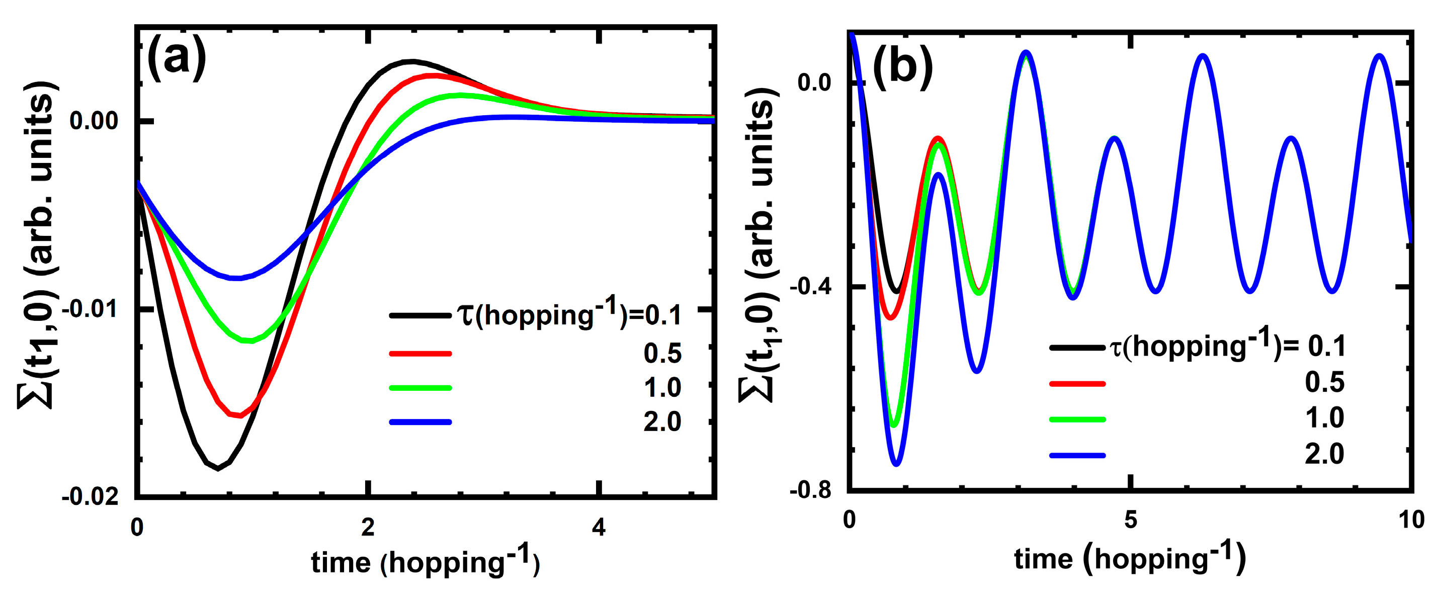
To give a feeling of the structure of the XC self-energy and hence of the XC potential, in Figure 2a we show results for for several pulse durations. We find that, for short pulses, the structure of is quite similar after the pulse time (Figure 2a), suggesting that the approximation for the XC potential might be meaningful.
6. Nonadiabatic XC Potential: Large-U Solution
In the case of large U, perturbation theory, Equations (64)–(68), can be also applied, but with (the expansion is performed in powers of dimensionless parameter ). Here, the main difference from the small U case is that the perturbation part of the Hamiltonian includes time explicitly, as modified by the Peierls substitution (82) for the hopping matrix elements.
In the first-order approximation, one then obtains (we consider the case with spin-diagonal GFs and self-energies):
and
Since we assume that the atomic GFs are local in space, one obtains:
and
i.e., the linear in-hopping part of the self-energy is zero.
In the second order, one finds:
and
or in the momentum representation:
(as expected, in the local-in-space approximation the self-energy is momentum-independent).
The result in Equation (112) is significantly simplified for a hypercubic lattice in which the free-electron spectrum and the two-energy DOS are defined by Equations (83) and (84), respectively. Note that one can perform the integration in Equation (112) exactly:
One thus obtains:
(we restored the dependence on U).
The atomic GF does not depend on hopping, thus there is no vector potential in this function and, hence, there is no time-dependence. Therefore, is the equilibrium GF.
Next, in the matrix representation, Equation (114) gives:
where
and the other two GFs are:
From Equations (115)–(120), one can obtain:
and
Together with Equations (98) and (99) for the small U case, Equations (124) and (125) for the case of strong interaction are the main results of this article. These equations define the XC potential (100) in the case of large Us. As in the case of weak interactions, here one can also calculate a spatial-local and a pulse-independent approximation, which gives However, contrary to the case of small U, the XC potential (124), (125) demonstrates oscillating behavior, with no signs of a finite memory time. The oscillations can be eliminated by using the adiabatic approximation, . However, this approximation gives a rather trivial XC potential (100) with time-independent time-ordered self-energy.
In Figure 2b, we show the time dependence of the greater self-energy (125) in the cases of different pulse durations. Again, as one can see from this figure, the details of the pulse become nonimportant at times longer than pulse, suggesting that the approximation is a meaningful one in this case as well.
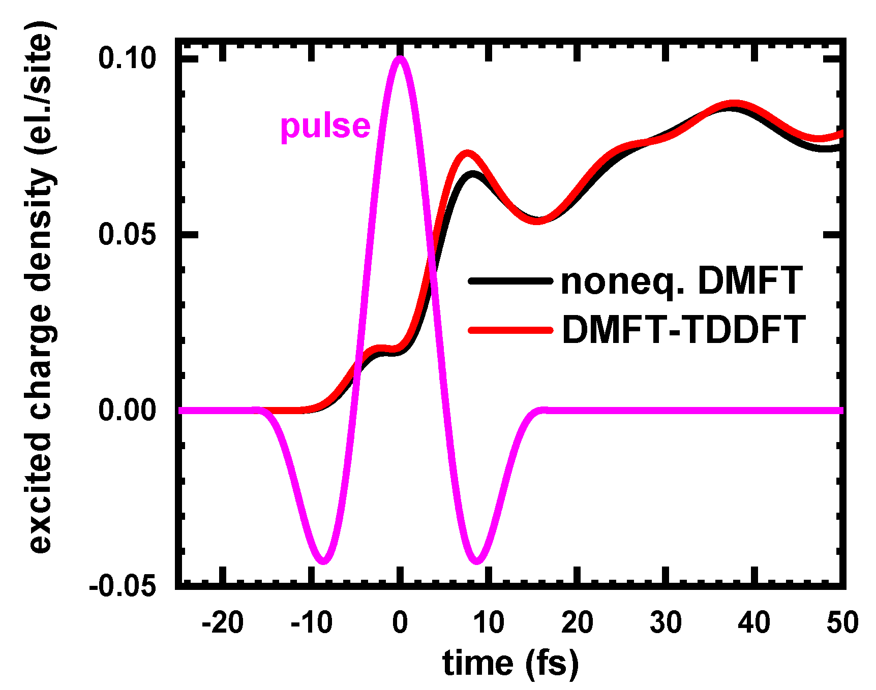
To test the kernel, we applied it to the half-filled one-band 3D Hubbard model at (in the more challenging case of a large U) in presence of an ultrafast laser pulse and compared the result for the time-dependent excited charge density with the corresponding results obtained with nonequilibrium DMFT (nonequilibrium iterative-perturbation theory solver). As it follows from the comparison displayed in Figure 3, the agreement between the results of nonequilibrium DMFT and DMFT-TDDFT is rather good. This is not surprising, since in both theories the time-dependence of the interacting dynamics is defined by basically the same function—nonequilibrium electron self-energy.
7. Summary and Future Directions
In this work, we have derived an analytical form of the time-ordered self-energy for the Hubbard model for both weak (Equations (95), (98) and (99)) and strong (Equations (95), (124) and (125)) local Coulomb repulsion. The obtained results were used to construct a nonadiabatic XC potential for strongly correlated systems (with an approximated form given in Equation (100)) by using the Sham–Schluter equation approach (below, we use notations and for the weak and strong interaction potentials, respectively). The only assumption used in the derivation of the self-energies was the locality of the GFs, in the spirit of DMFT.
Now that we have obtained potentials that correspond to the cases of weak and strong Coulomb interactions, the logical question is: how do we deal with the interesting case of intermediate U? The first attempt could be to use a hybrid potential , where . The value of the parameter would depend on whether the system is closer to the weak or strong correlation regimes or is between them ( (a more rigorous approach to define a weak–strong regime can be formulated in order to derive the value of the mixing parameter). A more rigorous approach is to solve the nonequilibrium DMFT problem and to find the self-energy in Equation (95) and to use it to construct the XC potential in Equation (100). Moreover, such a nonequilibrium numerical solution of the DMFT problem to construct the XC potential by using Equation (100), or more generally Equation (59), is necessary in the case of lattices different from the hypercubic one and/or in the multiband case, where it is not possible to obtain a simple analytical expression for the self-energy. The exact sum rules for the nonequilibrium self-energy [72,73] can be used to test the accuracy of the obtained potential. Since the multi-orbital nonequilibrium DMFT problem is computationally intensive, an effective one-orbital model (with the same values of U, average hopping and charge density per orbital) might be used to obtain . We tested the potential for the one-band Hubbard model and the obtained results that are encouraging.
It is important to mention that the potentials obtained are orbital potentials. There is thus the need to use a large enough number of orbitals in each particular case, depending on the width of the frequencies of the applied pulse. A convenient way to solve the corresponding TDDFT problem is the density matrix formalism (see, e.g., Ref. [74]). On the other hand, due to an analytical form of the time-dependent functions in the integral in the XC potential (Equation (100)), the computational cost of the approach is relatively low, comparable to other TDDFT methods (in particular, the calculation of the result shown in Figure 3 took approximately 2 h).
Another important point is the sum rules. Though we use a quasi-local local-in-space approximation (more accurately, our potential is orbital, not LDA), it is known that even local (TDLDA) XC potentials satisfy a very important exact sum rule—the harmonic potential theorem [75]. On the other hand, it is also known that in the case of exactly local nonadiabatic potentials, TDDFT might give contradictory results [76]. Since the potential in Equation (100) is not local in space, this issue should not arise. Nevertheless, many more tests of this functional are needed to obtain a better idea about its accuracy.
We expect the potentials can be used to analyze different properties of strongly correlated systems, including for novel materials such as nanoparticles and twisted bilayer graphene, from optical response to superconductivity (for the current status in the field, see Ref. [77]; though, in the superconducting case in addition to the derived “normal diagonal” self-energies one needs to add “nondiagonal” (Gorkov) self-energy parts, and the XC potential should also have more components (as discussed, e.g., by Gross and collaborators in Ref. [78] in the static case).
Several important tasks still need to be accomplished:
- (1)
- (2)
- To perform further analysis in order to understand the dependence of the XC potential on the external perturbation field and to make the potential “universal”, i.e., field-independent (putting A = 0 in the expressions for the self-energy can be regarded as the first attempt acceptable in the case of short pulses).
- (3)
- To integrate the role of phonons in the results for the spin-polarized case (see, e.g., Ref. [48]) to be able to apply the method to longer times.
- (4)
- To generalize the approach to the nonlocal case, i.e., to take into account the momentum-dependence of the XC self-energy [71].
- (5)
- To test the XC potentials by comparing the results with the ones obtained with the exact methods and with the experimental data.
Work in the above directions is in progress.
Author Contributions
Conceptualization, V.T. and T.S.R.; methodology, V.T. and T.S.R.; software, V.T.; validation, V.T. and T.S.R.; formal analysis, V.T.; writing—original draft preparation, V.T.; writing—review and editing, V.T. and T.S.R.; funding acquisition, T.S.R. All authors have read and agreed to the published version of the manuscript.
Funding
This research was partially funded by the US Department of Energy, grant number DE-FG02-07ER46354. We acknowledge the National Energy Research Scientific Computing Center (NERSC) for providing the computational resources (project m3612).
Institutional Review Board Statement
Not applicable.
Informed Consent Statement
Not applicable.
Data Availability Statement
All data that support the findings of this study are included within the article.
Conflicts of Interest
The authors declare no conflict of interest. The funders had no role in the design of the study; in the collection, analyses, or interpretation of data; in the writing of the manuscript; or in the decision to publish the results.
References
- Fulde, P. Electron Correlations in Molecules and Solids; Springer: Berlin/Heidelberg, Germany, 2002. [Google Scholar]
- Yamada, K. Electron Correlations in Metals; Cambridge University Press: Cambridge, UK, 2004. [Google Scholar]
- Anisimov, V.; Izyumov, Y. Electronic Structure of Strongly Correlated Materials; Springer: Berlin/Heidelberg, Germany, 2010. [Google Scholar]
- Wei, J.; Natelson, D. Nanostructure studies of strongly correlated materials. Nanoscale 2011, 3, 3509. [Google Scholar] [CrossRef] [PubMed]
- Liu, C.; Balin, I.; Magdassi, S.; Abdulhalim, I.; Long, Y. Vanadium dioxide nanogrid films for high transparency smart architectural window applications. Opt. Express 2015, 3, A124. [Google Scholar] [CrossRef] [PubMed]
- Nie, G.; Zhang, L.; Lei, J.; Yang, L.; Zhang, Z.; Lu, X.; Wang, C. Monocrystalline VO2 (B) nanobelts: Large-scale synthesis, intrinsic peroxidase-like activity and application in biosensing. J. Mater. Chem. A 2014, 2, 2910. [Google Scholar] [CrossRef]
- Rathi, S.; Park, J.-H.; Lee, I.-Y.; Baik, J.M.; Yi, K.S.; Kim, G.-H. Unravelling the switching mechanisms in electric field induced insulator–metal transitions in VO2 nanobeams. Phys. D Appl. Phys. 2014, 47, 295101. [Google Scholar] [CrossRef]
- Georges, A.; Kotliar, G.; Krauth, W.; Rozenberg, M.J. Dynamical mean-field theory of strongly correlated fermion systems and the limit of infinite dimensions. Rev. Mod. Phys. 1996, 68, 13. [Google Scholar] [CrossRef] [Green Version]
- Freericks, J.K.; Turkowski, V.M.; Zlatic, V. Nonequilibrium Dynamical Mean-Field Theory. Phys. Rev. Lett. 2006, 97, 266408. [Google Scholar] [CrossRef] [PubMed] [Green Version]
- Aoki, H.; Tsuji, N.; Eckstein, M.; Kollar, M.; Oka, T.; Werner, P. Nonequilibrium dynamical mean-field theory and its applications. Rev. Mod. Phys. 2014, 86, 779. [Google Scholar] [CrossRef] [Green Version]
- Hohenberg, P.; Kohn, W. Inhomogeneous Electron Gas. Phys. Rev. 1964, 136, B864. [Google Scholar] [CrossRef] [Green Version]
- Kohn, W.; Sham, L.J. Self-Consistent Equations Including Exchange and Correlation Effects. Phys. Rev. 1965, 140, A1133. [Google Scholar] [CrossRef] [Green Version]
- Runge, E.; Gross, E.K.U. Density-Functional Theory for Time-Dependent Systems. Phys. Rev. Lett. 1984, 52, 997. [Google Scholar] [CrossRef]
- Ullrich, C.A. Time-Dependent Density-Functional Theory: Concepts and Applications; Oxford University Press: Oxford, UK, 2011. [Google Scholar]
- Capelle, K.; Campo, V.L., Jr. Density functionals and model Hamiltonians: Pillars of many-particle physics. Phys. Rep. 2013, 528, 91. [Google Scholar] [CrossRef]
- Anisimov, V.I.; Aryasetiawan, F.; Lichtenstein, A.I. First-principles calculations of the electronic structure and spectra of strongly correlated systems: The LDA+ U method. J. Phys. Condens. Matter 1997, 9, 767. [Google Scholar] [CrossRef] [Green Version]
- Seidl, M.; Perdew, J.P.; Kurth, S. Simulation of All-Order Density-Functional Perturbation Theory, Using the Second Order and the Strong-Correlation Limit. Phys. Rev. Lett. 2000, 84, 5070. [Google Scholar] [CrossRef] [PubMed] [Green Version]
- Seidl, M.; Perdew, J.P.; Levy, M. Strictly correlated electrons in density-functional theory. Phys. Rev. A 1999, 59, 51. [Google Scholar] [CrossRef]
- Fabiano, E.; Śmiga, S.; Giarrusso, S.; Daas, T.J.; Della Sala, F.; Grabowski, I.; Gori-Giorgi, P. Investigation of the Exchange-Correlation Potentials of Functionals Based on the Adiabatic Connection Interpolation. J. Chem. Theory Comput. 2019, 15, 1006. [Google Scholar] [CrossRef] [PubMed]
- Lima, N.A.; Silva, M.F.; Oliveira, L.N.; Capelle, K. Density Functionals Not Based on the Electron Gas: Local-Density Approximation for a Luttinger Liquid. Phys. Rev. Lett. 2003, 90, 146402. [Google Scholar] [CrossRef] [PubMed] [Green Version]
- Lima, N.A.; Oliveira, L.N.; Capelle, K. Density-functional study of the Mott gap in the Hubbard model. Europhys. Lett. 2002, 60, 601. [Google Scholar] [CrossRef]
- Xianlong, G.; Polini, M.; Tossi, M.P.; Campo, V.L., Jr.; Capelle, K.; Rigol, M. Bethe ansatz density-functional theory of ultracold repulsive fermions in one-dimensional optical lattices. Phys. Rev. B 2006, 73, 165120. [Google Scholar] [CrossRef] [Green Version]
- Bergfield, J.P.; Liu, Z.-F.; Burke, K.; Staford, C.A. Bethe Ansatz Approach to the Kondo Effect within Density-Functional Theory. Phys. Rev. Lett. 2012, 108, 66801. [Google Scholar] [CrossRef] [Green Version]
- Campo, V.L. Density-functional-theory approach to the thermodynamics of the harmonically confined one-dimensional Hubbard model. Phys. Rev. B 2015, 92, 13614. [Google Scholar] [CrossRef] [Green Version]
- Hopjan, M.; Karlsson, D.; Ydman, S.; Verdozzi, C.; Almbladh, C.-O. Merging Features from Green’s Functions and Time Dependent Density Functional Theory: A Route to the Description of Correlated Materials out of Equilibrium? Phys. Rev. Lett. 2016, 116, 236402. [Google Scholar] [CrossRef] [PubMed] [Green Version]
- Senjean, B.; Nakatani, N.; Tsuchiizu, M.; Fromager, E. Site-occupation embedding theory using Bethe ansatz local density approximations. Phys. Rev. B 2018, 97, 235105. [Google Scholar] [CrossRef] [Green Version]
- Lieb, E.H.; Wu, F.Y. Absence of Mott Transition in an Exact Solution of the Short-Range, One-Band Model in One Dimension. Phys. Rev. Lett. 1968, 20, 1445. [Google Scholar] [CrossRef]
- López-Sandoval, R.; Pastor, G. Properties of the exact correlation-energy functional in Hubbard models. Ph. Transit. 2005, 78, 839. [Google Scholar] [CrossRef]
- Carrascal, D.; Ferrer, J. Exact Kohn-Sham eigenstates versus quasiparticles in simple models of strongly correlated electrons. Phys. Rev. B 2012, 85, 45110. [Google Scholar] [CrossRef] [Green Version]
- Xianlong, G.; Chen, A.-H.; Tokatly, I.; Kurth, S. Lattice density functional theory at finite temperature with strongly density-dependent exchange-correlation potentials. Phys. Rev. B 2012, 86, 235139. [Google Scholar] [CrossRef] [Green Version]
- Carrascal, D.; Ferrer, J.; Smith, J.C.; Burke, K. The Hubbard dimer: A density functional case study of a many-body problem. J. Phys. Condens. Matter. 2015, 27, 393001. [Google Scholar] [CrossRef] [Green Version]
- Liu, Z.-F.; Bergfield, J.P.; Burke, K.; Stafford, C.A. Accuracy of density functionals for molecular electronics: The Anderson junction. Phys. Rev. B 2012, 85, 155117. [Google Scholar] [CrossRef] [Green Version]
- Verdozzi, C. Time-Dependent Density-Functional Theory and Strongly Correlated Systems: Insight from Numerical Studies. Phys. Rev. Lett. 2008, 101, 166401. [Google Scholar] [CrossRef]
- Brosco, V.; Ying, Z.-J.; Lorenzana, J. Exact exchange-correlation potential of an ionic Hubbard model with a free surface. Sci. Rep. 2013, 3, 2172. [Google Scholar] [CrossRef] [Green Version]
- Pollack, L.; Perdew, J.P. Evaluating density functional performance for the quasi-two-dimensional electron gas. J. Phys. Condens. Matter 2000, 12, 1239. [Google Scholar] [CrossRef]
- Constantin, L.A. Dimensional crossover of the exchange-correlation energy at the semilocal level. Phys. Rev. B 2008, 78, 155106. [Google Scholar] [CrossRef] [Green Version]
- Constantin, L.A. Simple effective interaction for dimensional crossover. Phys. Rev. B 2016, 93, 121104. [Google Scholar] [CrossRef]
- Constantin, L.A. Correlation energy functionals from adiabatic connection formalism. Phys. Rev. B 2019, 99, 085117. [Google Scholar] [CrossRef]
- Lieb, E.H.; Seiringer, R.; Solovej, J.P. Ground-state energy of the low-density Fermi gas. Phys. Rev. A 2005, 71, 53605. [Google Scholar] [CrossRef] [Green Version]
- Giuliani, A. Ground state energy of the low density Hubbard model: An upper bound. J. Math. Phys. 2007, 48, 23302. [Google Scholar] [CrossRef] [Green Version]
- Seiringer, R.; Yin, J. Ground state energy of the low density Hubbard model. J. Stat. Phys. 2008, 131, 1139. [Google Scholar] [CrossRef]
- Bünemann, J.; Gebhard, F.; Weber, W. Gutzwiller-Correlated Wave Functions: Application to Ferromagnetic Nickel. In Frontiers in Magnetic Materials; Narlikar, A., Ed.; Springer: Berlin/Heidelberg, Germany, 2005. [Google Scholar]
- Schickling, T.; Bünemann, J.; Gebhard, F.; Weber, W. Gutzwiller density functional theory: A formal derivation and application to ferromagnetic nickel. New J. Phys. 2014, 16, 93034. [Google Scholar] [CrossRef] [Green Version]
- Giesbertz, K.J.H.; Uimonen, A.-M.; van Leeuwen, R. Approximate energy functionals for one-body reduced density matrix functional theory from many-body perturbation theory. Eur. Phys. J. B 2018, 91, 282. [Google Scholar] [CrossRef] [Green Version]
- Coe, J.P. Lattice density-functional theory for quantum chemistry. Phys. Rev. B 2019, 99, 165118. [Google Scholar] [CrossRef] [Green Version]
- Seidl, M. Strong-interaction limit of density-functional theory. Phys. Rev. A 1999, 60, 4387. [Google Scholar] [CrossRef]
- Karlsson, D.; Privitera, A.; Verdozzi, C. Time-Dependent Density-Functional Theory Meets Dynamical Mean-Field Theory: Real-Time Dynamics for the 3D Hubbard Model. Phys. Rev. Lett. 2011, 106, 116401. [Google Scholar] [CrossRef] [PubMed] [Green Version]
- Viñas Boström, E.; Helmer, P.; Werner, P.; Verdozzi, C. Electron-electron versus electron-phonon interactions in lattice models: Screening effects described by a density functional theory approach. Phys. Rev. Res. 2019, 1, 13017. [Google Scholar] [CrossRef] [Green Version]
- Nelson, J.; Tiwari, R.; Sanvito, S. Machine learning density functional theory for the Hubbard model. Phys. Rev. B 2019, 99, 75132. [Google Scholar] [CrossRef] [Green Version]
- Wang, L.W. Novel Computational Methods for Nanostructure Electronic Structure Calculations. Ann. Rev. Phys. Chem. 2010, 61, 19. [Google Scholar] [CrossRef]
- Gruner, M.E.; Entel, P. Competition between ordering, twinning, and segregation in binary magnetic 3d-5d nanoparticles: A supercomputing perspective. Int. J. Quant. Chem. 2012, 112, 277. [Google Scholar] [CrossRef]
- Schonhammer, K.; Gunnarsson, O.; Noack, R.M. Density-functional theory on a lattice: Comparison with exact numerical results for a model with strongly correlated electrons. Phys. Rev. B 1995, 52, 2504. [Google Scholar] [CrossRef]
- López-Sandoval, R.; Pastor, G.M. Density-matrix functional theory of the Hubbard model: An exact numerical study. Phys. Rev. B 2000, 61, 1764. [Google Scholar] [CrossRef] [Green Version]
- Aryasetiawan, F.; Gunnarsson, O. Exchange-correlation kernel in time-dependent density functional theory. Phys. Rev. B 2002, 66, 165119. [Google Scholar] [CrossRef]
- Wei, L.; Gao, X.L.; Kollath, C.; Polini, M. Collective excitations in one-dimensional ultracold Fermi gases: Comparative study. Phys. Rev. B 2008, 78, 195109. [Google Scholar]
- Fuks, J.I.; Maitra, N.T. Challenging adiabatic time-dependent density functional theory with a Hubbard dimer: The case of time-resolved long-range charge transfer. Phys. Chem. Chem. Phys. 2014, 16, 14504. [Google Scholar] [CrossRef] [PubMed] [Green Version]
- Fuks, J.; Maitra, N. Charge transfer in time-dependent density-functional theory: Insights from the asymmetric Hubbard dimer. Phys. Rev. A 2014, 89, 62502. [Google Scholar] [CrossRef] [Green Version]
- Lani, G.; di Marino, S.; Gerolin, A.; van Leeuwen, R.; Gori-Giorgi, P. The adiabatic strictly-correlated-electrons functional: Kernel and exact properties. Phys. Chem. Chem. Phys. 2016, 18, 21092–21101. [Google Scholar] [CrossRef] [PubMed] [Green Version]
- Turkowski, V.; Rahman, T.S. Nonadiabatic time-dependent spin-density functional theory for strongly correlated systems. J. Phys. Condens. Matter 2014, 26, 22201. [Google Scholar] [CrossRef] [Green Version]
- Mancini, L.; Ramsden, J.; Hodgson, M.; Godby, R. Adiabatic and local approximations for the Kohn-Sham potential in time-dependent Hubbard chains. Phys. Rev. B 2014, 89, 195114. [Google Scholar] [CrossRef] [Green Version]
- Turkowski, V.; Rahman, T.S. Nonadiabatic exchange-correlation kernel for strongly correlated materials. J. Phys. Condens. Matter 2017, 29, 455601. [Google Scholar] [CrossRef] [Green Version]
- Acharya, S.R.; Turkowski, V.; Zhang, G.P.; Rahman, T.S. Ultrafast Electron Correlations and Memory Effects at Work: Femtosecond Demagnetization in Ni. Phys. Rev. Lett. 2020, 125, 17202. [Google Scholar] [CrossRef]
- Sham, L.; Schlüter, M. Density-Functional Theory of the Energy Gap. Phys. Rev. Lett. 1983, 51, 1888. [Google Scholar] [CrossRef]
- van Leeuwen, R. The Sham-Schlüter equation in time-dependent density-functional theory. Phys. Rev. Lett. 1996, 76, 3610. [Google Scholar] [CrossRef]
- Turkowski, V.; Freericks, J.K. Nonequilibrium perturbation theory of the spinless Falicov-Kimball model: Second-order truncated expansion in U. Phys. Rev. B 2007, 75, 125110. [Google Scholar] [CrossRef] [Green Version]
- Vilk, Y.M.; Tremblay, A.-M.S. Non-Perturbative Many-Body Approach to the Hubbard Model and Single-Particle Pseudogap. J. Phys. Fr. 1997, 7, 1309. [Google Scholar] [CrossRef] [Green Version]
- Kusunose, H. Influence of Spatial Correlations in Strongly Correlated Electron Systems: Extension to Dynamical Mean Field Approximation. J. Phys. Soc. Jpn. 2006, 75, 54713. [Google Scholar] [CrossRef] [Green Version]
- Miyahara, H.; Arita, R.; Ikeda, H. Development of a two-particle self-consistent method for multiorbital systems and its application to unconventional superconductors. Phys. Rev. B 2013, 87, 45113. [Google Scholar] [CrossRef] [Green Version]
- Krieger, J.B.; Li, Y.; Iafrate, G.J. Derivation and application of an accurate Kohn-Sham potential with integer discontinuity. Phys. Lett. A 1990, 146, 256. [Google Scholar] [CrossRef]
- Hirata, S.; Ivanov, S.; Grabowski, I.; Bartlett, R.J.; Burke, K.; Talman, J.D. Can optimized effective potentials be determined uniquely? J. Chem. Phys. 2001, 115, 1635. [Google Scholar] [CrossRef]
- Rohringer, G.; Hafermann, H.; Toschi, A.; Katanin, A.A.; Antipov, A.E.; Katsnelson, M.I.; Lichtenstein, A.I.; Rubtsov, A.N.; Held, K. Diagrammatic routes to nonlocal correlations beyond dynamical mean field theory. Rev. Mod. Phys. 2018, 90, 25003. [Google Scholar] [CrossRef] [Green Version]
- Turkowski, V.; Freericks, J.K. Nonequilibrium sum rules for the retarded self-energy of strongly correlated electrons. Phys. Rev. B 2008, 77, 205102, Erratum in Phys. Rev. B 2010, 82, 119904. [Google Scholar] [CrossRef] [Green Version]
- Freericks, J.K.; Turkowski, V. Inhomogeneous spectral moment sum rules for the retarded Green function and self-energy of strongly correlated electrons or ultracold fermionic atoms in optical lattices. Phys. Rev. B 2009, 80, 115119, Erratum in Phys. Rev. B 2010, 82, 129902. [Google Scholar] [CrossRef] [Green Version]
- Turkowski, V.; Ud Din, N.; Rahman, T.S. Time-Dependent Density-Functional Theory and Excitons in Bulk and Two-Dimensional Semiconductors. Computation 2017, 5, 39. [Google Scholar] [CrossRef] [Green Version]
- Dobson, J. Harmonic-Potential Theorem: Implications for Approximate Many-Body Theories. Phys. Rev. Lett. 1994, 73, 2244. [Google Scholar] [CrossRef]
- Gross, E.K.U.; Kohn, V. Local density-functional theory of frequency-dependent linear response. Phys. Rev. Lett. 1985, 55, 2850, Erratum in Phys. Rev. Lett. 1986, 57, 923. [Google Scholar] [CrossRef] [PubMed]
- Spałek, J.; Fidrysiak, M.; Zegrodnik, M.; Biborski, A. Superconductivity in high-Tc and related strongly correlated systems from variational perspective: Beyond mean field Theory. Phys. Rep. 2022, 959, 1. [Google Scholar] [CrossRef]
- Lüders, M.; Marques, M.A.L.; Lathiotakis, N.N.; Floris, A.; Profeta, G.; Fast, L.; Continenza, A.; Massidda, S.; Gross, E.K.U. Ab initio theory of superconductivity. I. Density functional formalism and approximate functionals. Phys. Rev. B 2005, 72, 24545. [Google Scholar] [CrossRef] [Green Version]
Figure 1.
Schematic representation of approximations for the nonadiabatic XC potential for strongly correlated materials in the cases of different strengths of the external perturbation (nonlinearity) and different levels of importance of the memory effects. The approximated potentials (the two left and the right-bottom boxes) are obtained with DMFT. The general structure of the exact nonadiabatic XC potential (top right box) is not known.

Figure 2.
The real part of the greater XC self-energy for several values of the pulse duration: (a) small U (A = 1, U = 2, = 1, wherever it is appropriate, the units are hopping, or the inverse hopping) and (b) large U (A = 1, U = 6, = 2, n = 1.4, double occupancy = 0.1), obtained using Equations (104) and (125), respectively.

Figure 3.
DMFT-TDDFT vs. nonequilibrium DMFT solution for the time-dependent excited charge density in one-band 3D Hubbard model on cubic lattice at when the system is perturbed by pulse (magenta curve). In the DMFT-TDDFT case, the atomic hydrogen s-orbital wave functions were used for the DFT input.

Publisher’s Note: MDPI stays neutral with regard to jurisdictional claims in published maps and institutional affiliations. |
© 2022 by the authors. Licensee MDPI, Basel, Switzerland. This article is an open access article distributed under the terms and conditions of the Creative Commons Attribution (CC BY) license (https://creativecommons.org/licenses/by/4.0/).
Share and Cite
MDPI and ACS Style
Turkowski, V.; Rahman, T.S. Nonadiabatic Exchange-Correlation Potential for Strongly Correlated Materials in the Weak and Strong Interaction Limits. Computation 2022, 10, 77. https://0-doi-org.brum.beds.ac.uk/10.3390/computation10050077
AMA Style
Turkowski V, Rahman TS. Nonadiabatic Exchange-Correlation Potential for Strongly Correlated Materials in the Weak and Strong Interaction Limits. Computation. 2022; 10(5):77. https://0-doi-org.brum.beds.ac.uk/10.3390/computation10050077
Chicago/Turabian StyleTurkowski, Volodymyr, and Talat S. Rahman. 2022. "Nonadiabatic Exchange-Correlation Potential for Strongly Correlated Materials in the Weak and Strong Interaction Limits" Computation 10, no. 5: 77. https://0-doi-org.brum.beds.ac.uk/10.3390/computation10050077
Note that from the first issue of 2016, this journal uses article numbers instead of page numbers. See further details here.