
Preprocessing of Gravity Data


1
Department of Geodesy, University of Zilina, Univerzitna 8215/1, 010 26 Zilina, Slovakia
2
Department of Railway Engineering and Track Management, University of Zilina, Univerzitna 8215/1, 010 26 Zilina, Slovakia
*
Author to whom correspondence should be addressed.
Computation 2022, 10(6), 82; https://0-doi-org.brum.beds.ac.uk/10.3390/computation10060082
Submission received: 1 April 2022
/
Revised: 6 May 2022
/
Accepted: 18 May 2022
/
Published: 27 May 2022
Abstract
:The paper deals with computation techniques applied in preprocessing of gravity data, which are based on time series analysis by using mathematical and statistical smoothing techniques such as moving average, moving median, cumulative and moving average, etc. The main aim of gravity data preprocessing is to avoid abrupt errors caused by a sudden movement of the subsoil due to human or natural activities or systematic instrumental influences and so provide relevant gravity values, which are then subjected to further processing. The new approach of the described research involves the preprocessing phase in gravity data analysis to identify and avoid gross errors, which could influence the size of unknown parameters estimated by the least square method in the processing phase.
1. Introduction
Gravimetry is a science discipline used to provide important information about the earth’s geodynamical processes. Therefore, it is an integral part of almost all geosciences, including geophysics, geodesy, geology, geotechnics, etc. Gravity observations are useful for providing information on mass distribution within the earth or space, but they depend on time variation. Gravimetric measurements bring temporal gravity variations involving natural and human influences. These gravity variations can be recorded by the absolute or relative gravimeters, depending on particular technology and purpose. While absolute gravity measurements determine the gravity from the fundamental acceleration quantities and time, the modern, relative ones use a counterforce for the determination of gravity differences between different stations or, if carried out in the stationary mode, the variations of gravity with time [1]. The second mentioned observation method brings so-called stationary gravity values, organized in a time series dataset. The final gravity at the station depends on an instrument’s precision and the used processing method, which involves external and internal influences known as gravity corrections [2], instrumental drift, earth tides, and random noise. The precision of the reached gravity depends on identifying measurement errors and their subsequent reduction or elimination if possible. The raw gravity dataset, arranged in a time series, could be sometimes influenced by the sudden changes in readings brought by different causes: sudden earth movements, reading error, internal instrument effects, external influences, etc. These sudden changes in measured signals are called abrupt errors and are expressed as “jumping signals” in graphs.
The paper’s primary goal is to focus attention on the process of identification of abrupt errors of gravity data by using the mathematic-statistical technique used to be preferred mainly in financial engineering. The above-mentioned preprocessing analysis of time series data proceeds to the phase of creating a smoothed model, which is then submitted to further processing. The processing phase includes the minor gravity corrections involving external and internal influences on gravity data. It is not the main topic of the paper. Hence, it is mentioned only marginally at the end of the paper.
2. Time Series Analysis of Gravity Data
The preprocessing phase of gravity data consists of time series analysis to identify abrupt errors in the gravity dataset. Mathematics offers many tools to smooth such errors occurred in a continuous signal, from which methods of moving averages seem to be very useful. It belongs to the mathematic-statistical techniques that are useful for analyzing time series data, mainly in the trading world. In quantitative trading, time series analysis is about fitting statistical models, inferring underlying relationships between series or predicted future values, and generating trading signals. The method of time series analysis is a relatively old method, well described by many scientists like Anderson (1977), Kendall and Stuart (1979), Box, Brockwell (1991), Mongomery (1991), Jenkins and Reinsel (1994), Chatfield (1996), etc. [2,3,4,5,6,7,8]. It is applied by many users from various scientific disciplines, which operate with some quantity that is measured sequentially in time over some interval. In geodesy, time series analysis is often used to process long-term global navigation satellite system observations to determine earth and ocean tidal effects in a permanent station network.
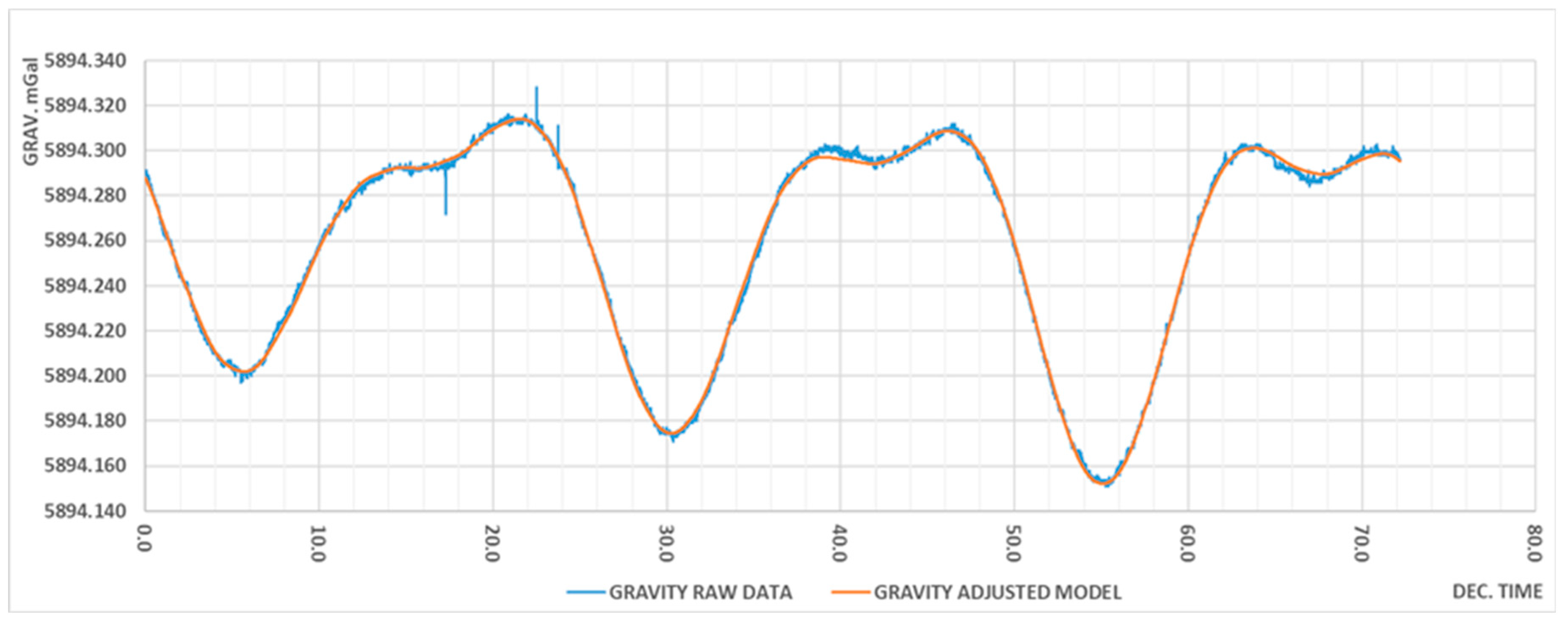
Some smoothing techniques have been applied to filter time series data to find the reliable function for cleaning up the raw gravity dataset (Figure 1). A moving average is an effective tool for adjusting a short-term time-series variation [9]. Several moving averages in time series analysis differ with the placement of the adjusted value. A simple “moving average” (MA) or one-sided moving average is placed at the end of values being averaged:
where index i changes from k + 1 to n, n is the number of data and k is the order or size of the sampling window. Two-sided MA is centered in the middle of the values being averaged:
where index i changes from k + 1 to n − k. While a two-sided moving average can estimate or see the trend, the one-sided moving average can be used as a simple forecasting method. Both types of moving averages use an odd number of periods. However, when working with time series, seasonality effects must be smoothed, which requires the period to be equal to seasonal length. “Centred moving average” (CMA) is often applied for this purpose, which distinguishes from others by using an even number of values:
If the user wants to get the average of all data up until the current datum point, “cumulative moving average” (CuMA) is suitable. In CuMA, the data arrive in an ordered datum stream, and the user would like to get the average of all of the data up until the current datum point
where t changes from 1 to n. In the case of robust statistics, “Moving median” (MM) is the most suitable to smooth or remove the time series noise. The moving median is not so popular as the moving average, but it provides a more robust estimate of a trend compared to the moving average. It is not affected by outliers, and it removes them. The moving median in a sampling window is calculated from linear approximation defined in the interval:
and is defined as robust statistics corresponding to 50% quantile (α = 0.5):
An overview of the values of the particular moving averages at critical points of gravity dataset is in Table 1, in which the column SMOOTHED GRAV. represents the adjusted data estimated by the least-squares method
“Weighted moving average” (WMA) is often applied in technical analysis of financial data with the specific meaning of weights that decrease arithmetical progression. In a p-day of WMA, the latest day has weight p, the second latest p − 1, etc., down to one:
where index i means the time and p is the weight. The weighted moving average has not been applied in the smoothing analysis of gravity data because of the unreasoning use of weights in gravity time series.
“Exponential moving average” (EMA) is also weighted toward the most recent value, but the rate of decrease between one value and its preceding value is not consistent. The difference in the decrease is exponential. The formula for EMA [10] is as follows:
where k changes from 0 to n. The weight of the general datum point is . WMA and EMA techniques seem to be more suitable for comparing more grav observed in various time intervals.
3. Abrupt Error Identifying
Scientists use many methods to identify outliers or gross errors in observation. Most of them utilize statistical hypothesis testing based on comparing the testing value with the critical one, which is represented by the quantile of a probability distribution. Abrupt error is assumed to be an outlier of the gravity dataset, which is indicated by comparing the corresponding residual value with the critical value estimated from the equation:
where σGRAV is the standard deviation of gravimeter SCINTREX Autograv CG-5 [13] defined by producer by the value 0.5 mGal and t is a confidential coefficient defined as a quantile of Student distribution dependent on specified probability. Quantitatively is t equal to 2.
Experimental measurements were obtained from three days of static observation of gravity acceleration realized by autograph with the setup read time of 60 s, which responded to 4331 observation cycles. From the Autograv optional parameters, tide and terrain corrections have been disallowed to perform the requisite functions in the processing phase.
Statistical hypothesis testing has been applied to confirm the existence of the abrupt error. It compares the testing value represented by the corresponding residual ei (Table 2) with the critical value Tα = 0.010 mGal by defining the probability value p = 0.95. As illustrated in Figure 1, three abrupt errors have been identified in the gravity dataset with the appropriate values of residuals and moving averages.
4. Regression Function as the Smoothing and Estimating Function
The smoothed method depends on the amount and character of time series data or the operator’s possibilities and preferences. However, the simplest way to avoid the abrupt error seems to be to apply the reliable smoothing and estimating technique to adjust raw gravity data and estimate the unknown parameters. Time series gravity data assumes to use nonlinear regression function used to estimate unknown parameters. The advantage of combining both moving average and regression function in gravity dataset (Figure 1) leads to computation of the reliable earth tide parameters from the mathematical model:
where Δg0, g1, g2, g3 are estimated unknown parameters of a gravimeter drift a, b, c, d are unknown parameters of earth tides depending on time changes ti − t0, which are needed to compute amplitude Ai and phase pi of a particular tidal wave with its period Ti according to the following formulas [14]:
The appropriate coefficients of gravimeter drift, the earth tides parameters estimated by the periods T1 = 1.075806 and T2 = 0.517525 defined for tidal wave components O1 and M2, and calculated values of amplitude and phase are displayed in Table 3.
The last symbol of Equation (10) represents a random gravitational noise that can be linear or harmonic, in nature and represents the unused rest of the harmonic series. The unknown regression parameters as the drift and tidal parameters of gravity data and their relevant variance components were estimated by the least square method.
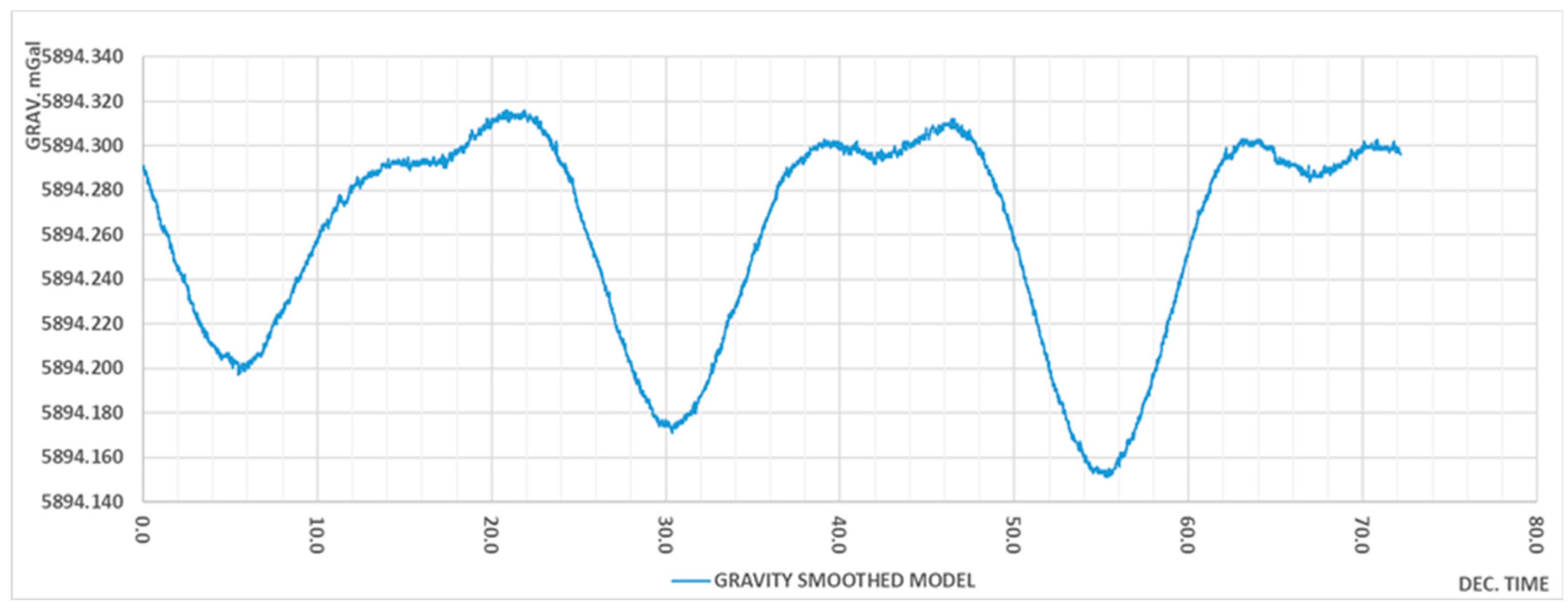
The gravity preprocessing finishes with the creation of the smoothed gravity model, displayed in Figure 2, which was prepared for the data processing to apply nominal gravity corrections.
5. Discussion
The paper‘s main topic is to apply the reliable smoothing technique for the time series analysis of the gravity dataset. While the moving average, moving median, and centred moving average seems to be very useful in the process of gross error identification, the cumulative moving average appears to be not so sensitive to smooth abrupt errors in the gravity data. Weighted and exponential smoothing techniques appear to be not suitable to use in gravity data preprocessing. Mathematics provides another smoothing technique based on data adjustment and estimation. The most suitable for gravity data seems to be the nonlinear regression with the least square restriction.
6. Conclusions
The smoothed gravity model was then subjected to the implementation of the nominal gravity corrections to find out the mathematical model of gravity acceleration at the station. The processing phase consists of involving external and internal influences represented by earth and ocean tides, hydrogeological forces, atmospheric pressure and temperature changes, seismic and terrain corrections, tilt and calibration corrections, and instrumental drift, which occurs due to the stress relaxation in the elastic quartz system of modern relative gravimeters. The most mathematical model involves random noise, representing random disturbances of gravity data.
Besides the mentioned effects, other disturbances influence the actual gravity acceleration value at the station as polar motion, instrument and station origin, earthquakes, tectonics, etc. Most of these influences are system parameters and are involved as firmware filters.
The widely used processing method of gravity data is a remove-restore technique [15,16]. This general method of gravity data processing is based on two phases. The first one, called the remove phase, is based on making nominal corrections for the largest influences, such as tides and pressure. Then, the problems are fixed in the residual signal and returned to the removed signals in the second restore phase.
Another approach to gravity data preprocessing seems to be finding the causes of abrupt error occurrences, which can have various origins consisting of external, instrumental, or human sources.
Author Contributions
Practical outputs, solution, analysis, D.B. and J.C.; Conceptualization, S.H.; Methodology, writing J.I.; All authors have read and agreed to the published version of the manuscript.
Funding
This research was funded by Ministry of education, science, research and sporz of the Slovak Republic, grant number: VEGA 1/0643/21.
Institutional Review Board Statement
Not applicable.
Data Availability Statement
There is only a part of data from own direct measurements in the manuscript. No conflict with their using.
Acknowledgments
This article is the result of the implementation of the project VEGA 1/0643/21, “Analysis of spatial deformations of a railway track observed by terrestrial laser scanning”, supported by the Scientific Grant Agency of the Ministry of Education, Science, Research and Sport of the Slovak Republic and Slovak Academy of Sciences. This article is the result of implementing the project KEGA 038ŽU-4/2020,“New approaches to teaching physical geodesy in higher education”, supported by the Scientific Grant Agency of the Ministry of Education, Science, Research and Sport of the Slovak Republic.
Conflicts of Interest
The authors declare no conflict of interest.
References
- Torge, W. Gravimetry; Walter de Gruyter: Berlin, Germany; New York, NY, USA, 1989; 465p, ISBN 3110107023. [Google Scholar]
- Lederer, M. Accuracy of the relative gravity measurements. Acta Geodyn. Geomater. 2009, 6, 383–390. [Google Scholar]
- Anderson, O.D. Time series analysis and forecasting: Another look at the Box-Jenkins approach. J. R. Stat. Soc. 1977, 26, 285–303. Available online: https://0-www-jstor-org.brum.beds.ac.uk/stable/2987813 (accessed on 1 January 2020). [CrossRef]
- Kendall, M.; Stuart, A. The Advanced Theory of Statistics—Volume 2: Inference and Relationship; Charles Griffin & Co. Limited: London, UK, 1979; 736p. [Google Scholar]
- Box, G.E.P.; Jenkins, G.M.; Reinsel, G.C. Time Series Analysis, 4th ed.; John Wiley & Sons, Inc.: Hoboken, NJ, USA, 2008; 746p, ISBN 9781118619193. [Google Scholar]
- Brockwell, P.J.; Davis, R.A. Time-Series: Theory and Methods; eBook; Springer: Berlin, Germany, 1991; 577p, ISBN 978-1-4419-0320-4. [Google Scholar]
- Montgomery, D.C. Design and Analysis of Experiments, 8th ed.; John Wiley & Sons: New York, NY, USA, 2013; 724p. [Google Scholar]
- Chatfield, C. The Analysis of Time Series—An Introduction, 5th ed.; Chapman and Hall CRC: London, UK, 2003; 352p. [Google Scholar]
- e-Handbook of Statistical Methods, NIST/SEMATECH. 2012. Available online: http://www.itl.nist.gov/div898/handbook/ (accessed on 24 April 2012).
- Hunter, J.S. The Exponentially weighted moving average. J. Qual. Technol. 2018, 18, 203–210. [Google Scholar] [CrossRef]
- El-Habiby, M.; Sideris, M.G. On the Potential of Wavelets for Filtering and Thresholding Airborne Gravity Data; The University of Calgary, 2500 University Drive, N.W.: Calgary, AB, Canada. Available online: https://www.isgeoid.polimi.it/Newton/Newton_3/El-Habiby.pdf (accessed on 21 January 2006).
- Zhao, L.; Wu, M.; Forsberg, R.; Olesen, A.V.; Zhang, K.; Caou, J. Airborne Gravity Data Denoising Based on Empirical Mode Decomposition: A Case Study for SGA-WZ Greenland Test Data. ISPRS Int. J. Geo-Inf. 2015, 4, 2205–2218. [Google Scholar] [CrossRef] [Green Version]
- Scintrex. CG-5 Operational Manual; Scintrex System—Part #867700 Revision 8; Scintrex: Concord, ON, Canada, 2012. [Google Scholar]
- Vanicek, P. The Earth Tides; Lecture Notes No. 36; University of New Brunswick: Fredericton, NB, Canada, 1973; p. 38. [Google Scholar]
- Torge, W.; Jürgen, M. Geodesy; De Gruyter: Berlin, Germany, 2012; 433p, ISBN 978-3-11-020718-7. [Google Scholar]
- Wellenhof, B.H.; Moritz, H. Physical Geodesy; Springer: Vienna, Austria; New York, NY, USA, 2006; 403p, ISBN 10 3-211-33544-7. [Google Scholar]
Figure 1.
Time series of gravity dataset (original figure).

Figure 2.
Smoothed gravity model (original figure).


Table 1.
A demonstration of the sensitivity of the particular smoothing techniques.
| DAY | RAW GRAV. | MA | CMA | CuMA | MM | SMOOTHED GRAV. |
|---|---|---|---|---|---|---|
| 0.7192 | 5894.2870 | 5894.2900 | 5894.2920 | 5894.2530 | 5894.2900 | 5894.2870 |
| 0.7200 | 5894.2720 | 5894.2830 | 5894.2530 | 5894.2870 | 5894.2910 | |
| 0.7207 | 5894.2930 | 5894.2840 | 5894.2860 | 5894.2530 | 5894.2870 | 5894.2930 |
| 0.7215 | 5894.2950 | 5894.2870 | 5894.2530 | 5894.2930 | 5894.2950 | |
| 0.7222 | 5894.2940 | 5894.2940 | 5894.2880 | 5894.2530 | 5894.2940 | 5894.2940 |
| 0.9374 | 5894.3100 | 5894.3100 | 5894.3110 | 5894.2660 | 5894.3100 | 5894.3100 |
| 0.9381 | 5894.3280 | 5894.3160 | 5894.2660 | 5894.3110 | 5894.3140 | |
| 0.9389 | 5894.3100 | 5894.3160 | 5894.3150 | 5894.2660 | 5894.3100 | 5894.3100 |
| 0.9396 | 5894.3110 | 5894.3160 | 5894.2660 | 5894.3110 | 5894.3110 | |
| 0.9404 | 5894.3110 | 5894.3110 | 5894.3150 | 5894.2660 | 5894.3110 | 5894.3110 |
| 0.9885 | 5894.3020 | 5894.2980 | 5894.2970 | 5894.2680 | 5894.2960 | 5894.3020 |
| 0.9893 | 5894.3110 | 5894.3030 | 5894.2680 | 5894.3020 | 5894.3010 | |
| 0.9900 | 5894.2920 | 5894.3020 | 5894.3010 | 5894.2680 | 5894.3020 | 5894.3010 |
| 0.9908 | 5894.2950 | 5894.2990 | 5894.2680 | 5894.2950 | 5894.3010 | |
| 0.9916 | 5894.2950 | 5894.2940 | 5894.2990 | 5894.2680 | 5894.2950 | 5894.3000 |
| Mean square error in mGal | 0.0009 | 0.0011 | 0.0468 | 0.001 | 0.0027 | |
Table 2.
An overview of the particular residuals estimated at critical points in the time series.
| DAY | RAW GRAV. | eMA | eCMA | eCuMA | eMM | eSMOOTH |
|---|---|---|---|---|---|---|
| 0.7192 | 5894.2870 | −0.0039 | −0.0049 | 0.0338 | −0.003 | −0.0039 |
| 0.7200 | 5894.2720 | −0.0189 | 0.0188 | −0.015 | −0.0189 | |
| 0.7207 | 5894.2930 | 0.0020 | 0.0075 | 0.0397 | 0.0060 | 0.0020 |
| 0.7215 | 5894.2950 | 0.0039 | 0.0417 | 0.0020 | 0.0039 | |
| 0.7222 | 5894.2940 | 0.0029 | 0.0064 | 0.0407 | 0.0000 | 0.0029 |
| 0.9374 | 5894.3100 | −0.0043 | −0.0005 | 0.0443 | 0.0000 | −0.0043 |
| 0.9381 | 5894.3280 | 0.0138 | 0.0623 | 0.0170 | 0.0138 | |
| 0.9389 | 5894.3100 | −0.004 | −0.0048 | 0.0442 | 0.0000 | −0.004 |
| 0.9396 | 5894.3110 | −0.0029 | 0.0452 | 0.0000 | −0.0029 | |
| 0.9404 | 5894.3110 | −0.0028 | −0.0039 | 0.0452 | 0.0000 | −0.0028 |
| 0.9885 | 5894.3020 | 0.0006 | 0.0048 | 0.0343 | 0.0060 | 0.0006 |
| 0.9893 | 5894.3110 | 0.0099 | 0.0433 | 0.0090 | 0.0099 | |
| 0.9900 | 5894.2920 | −0.0088 | −0.0087 | 0.0242 | −0.01 | −0.0088 |
| 0.9908 | 5894.2950 | −0.0056 | 0.0272 | 0.0000 | −0.0056 | |
| 0.9916 | 5894.2950 | −0.0053 | −0.0041 | 0.0272 | 0.0000 | −0.0053 |
Table 3.
Tidal parameters estimated in gravity model (8).
| ∆g | g1 | g2 | g3 | a | b | c | d | A | p |
| 5894.269 | −0.000193 | −0.000004 | 0.000000 | −0.004785 | −0.028121 | −0.013337 | 0.021867 | 0.028525 | 1.402253 |
Publisher’s Note: MDPI stays neutral with regard to jurisdictional claims in published maps and institutional affiliations. |
© 2022 by the authors. Licensee MDPI, Basel, Switzerland. This article is an open access article distributed under the terms and conditions of the Creative Commons Attribution (CC BY) license (https://creativecommons.org/licenses/by/4.0/).
Share and Cite
MDPI and ACS Style
Izvoltova, J.; Bacova, D.; Chromcak, J.; Hodas, S. Preprocessing of Gravity Data. Computation 2022, 10, 82. https://0-doi-org.brum.beds.ac.uk/10.3390/computation10060082
AMA Style
Izvoltova J, Bacova D, Chromcak J, Hodas S. Preprocessing of Gravity Data. Computation. 2022; 10(6):82. https://0-doi-org.brum.beds.ac.uk/10.3390/computation10060082
Chicago/Turabian StyleIzvoltova, Jana, Dasa Bacova, Jakub Chromcak, and Stanislav Hodas. 2022. "Preprocessing of Gravity Data" Computation 10, no. 6: 82. https://0-doi-org.brum.beds.ac.uk/10.3390/computation10060082
Note that from the first issue of 2016, this journal uses article numbers instead of page numbers. See further details here.