
One-Dimensional Thermomechanical Model for Additive Manufacturing Using Laser-Based Powder Bed Fusion


School of Technology, JAMK University of Applied Sciences, P.O. Box 207, 40101 Jyväskylä, Finland
*
Author to whom correspondence should be addressed.
Computation 2022, 10(6), 83; https://0-doi-org.brum.beds.ac.uk/10.3390/computation10060083
Submission received: 7 April 2022
/
Revised: 12 May 2022
/
Accepted: 24 May 2022
/
Published: 27 May 2022
Abstract
:We investigate the thermomechanical behavior of 3D printing of metals in the laser-based powder bed fusion (L-PBF) process, also known as selective laser melting (SLM). Heat transport away from the printed object is a limiting factor. We construct a one-dimensional thermoviscoelastic continuum model for the case where a thin fin is being printed at a constant velocity. We use a coordinate frame that moves with the printing laser, and apply an Eulerian perspective to the moving solid. We consider a steady state similar to those used in the analysis of production processes in the process industry, in the field of research known as axially moving materials. By a dimensional analysis, we obtain the nondimensional parameters that govern the fundamental physics of the modeled process. We then obtain a parametric analytical solution, and as an example, illustrate it using material parameters for 316L steel. The nondimensional parameterization has applications in real-time control of the L-PBF process. The novelty of the model is in the use of an approach based on the theory of axially moving materials, which yields a new perspective on modeling of the 3D printing process. Furthermore, the analytical solution is easy to implement, and allows fast exploration of the parameter space.
1. Introduction
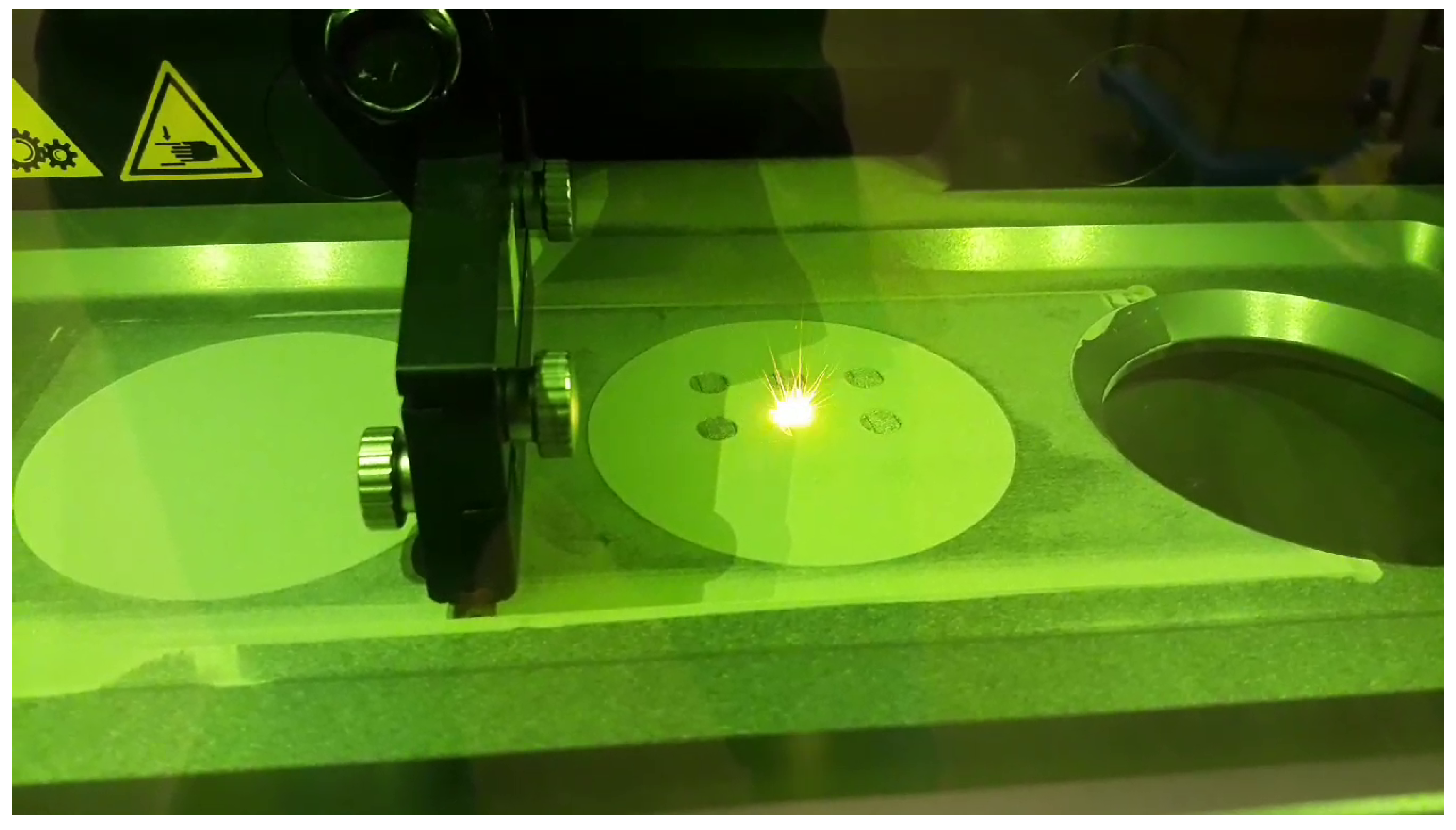
In the recent years, additive manufacturing processes for metals, including powder bed fusion (PBF) processes, have become a focus of both computational and experimental research. Additive manufacturing is attractive, because it provides the possibility to manufacture shapes not achievable by other methods [1], as well as offers operational flexibility and reduced production time [2]. In this study, we concentrate on laser-based powder bed fusion (L-PBF), also known as selective laser melting (SLM), see Figure 1.
Once a design is fed to the printer, the physical printing process begins by applying a thin layer of metal powder to the top of a solid baseplate, which forms the printable area. A laser then selectively heats the powder layer, melting the metal along the laser’s path. As the liquefied metal cools off and becomes solid, it fuses together, thus forming the first layer of the 3D printed object. Then another layer of powder is applied on top of the completed layer, and the melting process repeats for that layer. The second layer fuses onto the top of the first, and so on. Layer by layer, the printed object takes shape. In each layer, any powder that is not part of the shape being printed is left unused in the printable area, and must be removed once the printing is complete [1,3].
There are two avenues of research that have particularly received the attention of researchers in additive manufacturing of metal products. One is the characterization of the thermal response, and the other is the investigation of the effects of various process parameters and postprocessing techniques on the mechanical properties of the end product. In the following, we present some examples of each.
For example, de Moraes and Czekanski [4] studied the effects of the properties of the metal powder, such as grain diameter and packing density, on its thermal conductivity in the L-PBF process. In [5], the same authors considered the effects of laser power input on the thermal response of the material, using a transient finite element model.
Mirkoohi et al. [6] considered a multi-layer model for the temperature distribution in a semi-infinite solid during additive manufacturing, using a moving heat source approach. Irwin and Michaleris [7] suggested a line scan technique as a performance optimization for the classical moving heat source approach.
Denlinger et al. [3] considered the thermal response during the L-PBF process. The authors modeled both the powder and the solidified material, and observed that heat conduction into the powder bed is a significant heat transport mechanism. The authors ran variants of the model both with and without the powder, and concluded that the predicted temperatures are over 30% higher when the powder is not included in the simulation. The more complete model, which includes the powder, was found to better match experimental results.
Gusarov and Kovalev [8] investigated the thermal conductivity of the powder bed, considering the heat transfer both through contacts between spherical powder grains in various packing configurations, as well as across the gas gaps between them.
As for studies on the properties of the end product, Peng et al. [2] reviewed post-processing technologies in additive manufacturing, particularly in relation to improving the surface quality of the manufactured parts. Kahl et al. [9] suggested a computationally lightweight thermal model for real-time control of laser metal deposition, incorporating also data from a thermal camera. Kiran et al. [10] developed a thermomechanical model for residual stress prediction in the directed energy deposition (DED) process, which is an alternative to PBF.
Lu et al. [11] pointed out that residual stresses are one of the primary causes behind crack propagation and structural distortion, which lead to mechanical failure. The authors set out to uncover the mechanism that produces residual stresses in end products of additive manufacturing, noting that classically, residual stress mitigation in AM products has concentrated on the reduction of thermal gradients, although it has not been shown whether or not this is a significant contributor to residual stresses. They found that in the inner part of the printed product, reduction of the maximum thermal gradient produces satisfactory results, but in the first layers near the baseplate, decreasing the mechanical restraint between the baseplate and the printed material is more effective.
As for studies concentrating specifically on the end products of L-PBF, Sotiriou et al. [12] developed a coupled transient thermomechanical and microstructural model of the L-PBF process, determining the distribution of phases and alloying elements, and their effects on the mechanical properties of the end product.
Mokhtari et al. [13] considered the possibility of welding parts produced by L-PBF to overcome the size limitation of the manufacturing technique, and experimentally investigated the mechanical properties of the resulting welded product, comparing to a corresponding product welded from cold-rolled steel.
Letenneur et al. [14] investigated the density of the printed material produced in the L-PBF process. In the analysis, the authors combined the effect of the melt pool dimensions predicted by modeling, as well as the effects of laser power, scanning speed, hatching space, and layer thickness, which were accounted for experimentally. Kreitcberg et al. [15] reported experimental results concerning the microstructure and mechanical properties of an alloy processed by the L-PBF process and then subjected to post-treatment.
In the present study, we concentrate on the thermomechanical behavior of the L-PBF process. Heat transport away from the printed object is a limiting factor. As Milewski [1] has pointed out, in some cases it is necessary to print temporary support structures, not to support the weight of the upper layers, but to efficiently conduct heat away from them.
As is evident from the studies cited above, modeling the thermomechanical behavior of an object being printed by L-PBF is a complex task. The previous layer, on top of which the current layer is being printed, consists partly of the solidified printed object, and partly of unused powder. The already solidified part of the printed object is still hot, affecting the cooling of the current layer, while the powder technically is a viscous fluid consisting of macroscopic particles, in its undisturbed state, it can be considered as a porous solid, which transports heat primarily by conduction. The material properties depend on temperature, and the process involves a large range of temperatures, from room temperature up to the melting point of the metal.
With the goal of producing an analytical solution, we construct a radically simplified thermomechanical continuum model. To expose the fundamental phenomena, we abstract away the geometry of the design being printed, and consider printing in a straight line, at a constant velocity. This corresponds to printing a vertical thin fin. The setup shares some similarities with continuous casting; see, e.g., the study by Risso et al. [16].
In an actual L-PBF device, the laser scans a stationary material. Therefore, to an observer looking at the printable area, the temperature and displacement fields of the metal vary in time. However, if we switch to an Eulerian perspective, where our observer follows the focus spot of the laser, then some configurations, such as the one considered here, admit a non-stationary steady state, where temperature and displacement stay constant in time from the viewpoint of that observer even as the printing process proceeds.
The Eulerian perspective allows us to view the printing as a continuous process, and possibly see features that would be otherwise missed. A similar approach has been employed by Bugeda et al. [17] to the analysis of selective laser sintering, a relative of L-PBF without full melting, but to our knowledge, it has not been applied specifically to L-PBF.
In this study, we apply the approach from a theoretical perspective, and solve a simplified model analytically, to expose the fundamental behavior of the process. We leave open the expansion into more detailed computational and experimental studies later. This systematic approach allows the present study to act as a point of comparison, to clearly display which effects are introduced by each specific refinement of the model.
Traditionally, an Eulerian perspective to traveling solids has been extensively used in the process industry, for example the making of steel, textiles and paper. The first study to take this perspective was by Skutch [18], on the transverse vibrations of a string axially moving through two pinholes. The modern reader may want to look at the paper by Salonen and Koivurova [19]. The body of research is known as axially moving materials, or axially moving continua. Many specific studies concentrate on specific types of axially moving continua such as strings, membranes, beams, panels, or plates. A detailed introduction of the topic is beyond the scope of this paper; see for example Banichuk et al. ([20] ch. 5) for further references on some important avenues of research, and a systematic first-principles derivation of the equations of free vibration of an axially moving panel.
In this study, we consider only the region where the metal has solidified. Thus, the focus is more sharply on the printed material, when compared to existing studies, such as the aforementioned papers by Denlinger et al. [3], Sotiriou et al. [12], and de Moraes and Czekanski [5], in which the whole system was modeled, including the laser heat input.
We ignore the gap in the solidus and liquidus temperatures, and model the transition from liquid to solid as instantaneous, occurring when the temperature falls below a unique melting point. Since the analysis includes just one phase, we ignore the phase transition enthalpy; at all points in the solidified region, that energy has already dissipated. We treat material parameters as constants. Particularly, their dependence on temperature is ignored.
We use small-displacement kinematics, and the Kelvin–Voigt viscoelastic material model. We leave open the possibility for expansion in future studies, such as to the standard linear solid (SLS/Zener), and to nonlinear viscoplastic models such as those of the Chaboche family.
The rest of the paper is laid out as follows. After first introducing our problem setup, we discuss the governing equations. Then we specialize the equations into a steady state in one space dimension. We then solve the thermal problem, and then the mechanical problem, leading to a parametric analytical solution of the complete thermomechanical problem. We conclude with numerical examples, followed by a short discussion of the results and future directions.
The novelty of the model is in the use of an approach based on the theory of axially moving materials, which yields a new perspective on modeling of the 3D printing process. By a dimensional analysis, we have found the seven nondimensional parameters that govern the fundamental physics of the 3D printing process. Furthermore, the analytical approach lends itself to fast and efficient numerical solution, which has applications in real-time prediction and control.
2. Problem Setup
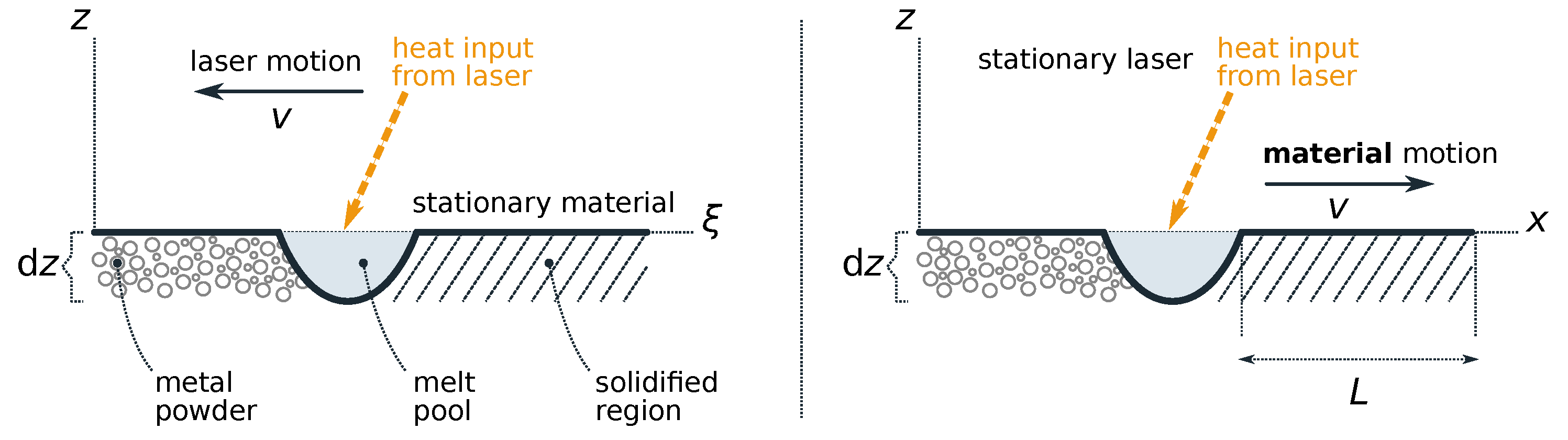
Consider the L-PBF process operating in a straight line. The laser scans toward the left, at a constant speed v, see Figure 2. By Galilean relativity, we consider the laser as remaining stationary, and the material as moving toward the right, at the same constant speed v. This allows us to apply the mixed Lagrangean–Eulearian formulation of axially moving materials [19]. We first consider the general dynamic situation, and then specialize to a steady state for the Eulerian observer.
For the Eulerian domain length L, unlike in typical process industry applications, in the present problem there is only one natural boundary that is stationary in the frame: the trailing edge of the melt pool, where the axially moving material enters the solidified region. The model thus naturally describes a semi-infinite solid. We place the trailing edge of the melt pool at . The other boundary, or in other words, the value of L, we may choose in whichever way it best facilitates our analysis.
It is useful to make L larger than the diameter of the printing area in a typical 3D printer, to see the fundamental physics of the undisturbed process up to thermal and mechanical equilibrium. We will later find that a natural way to choose L to facilitate this is to consider the ratio of timescales of different physical subprocesses; particularly, the time it takes a material parcel to travel through the domain (i.e., ), versus a characteristic cooling time.
By a material parcel, we refer to the continuum mechanics concept of a very small, essentially pointlike connected subset of the continuum material, but nevertheless large enough to exhibit macroscopic properties, such as density and temperature.
3. Governing Equations
To build our continuum model, we specify its three fundamental parts: balance laws, kinematic relations, and constitutive relations. Before reduction into one dimension, we develop the model in a tensor format. We use cartesian tensors, or in other words, we work in an orthonormal coordinate system, thus ignoring the metric, and the distinction between contravariant and covariant tensor components.
As the starting point, in tensor form, the continuum balance laws we need are (see, e.g., Allen et al. [21]) the balance of linear momentum,
and the balance of specific internal energy,
In Equation (1), is the density of the material (with SI unit ), is the material parcel velocity (), is the material derivative associated with the velocity field , is the stress tensor (), is a specific body force (), and is the transpose of a rank-2 tensor.
In Equation (2), e is the specific internal energy (), is the heat flux (; note the sign convention matching that of Allen et al. [21]; means heat flows into the material parcel), and h is an external specific heat source ().
For the symbol ∇, we use the prefix-partial (a.k.a. transpose jacobian) convention, which in a cartesian setting allows treating ∇ as a vector: . For example, the directional derivative is , and the gradient of a vector is . The dot product denotes the single contraction, and the double-dot product denotes the double contraction, no swap: .
Using Fourier’s law and the constitutive law of specific internal energy for a situation with no phase transitions, , Equation (2) becomes the generalized heat equation,
In Equation (3), c is the specific heat capacity (), T is the temperature (), and is the heat conductivity tensor (rank 2; ).
In the mixed Lagrangean–Eulerian description, the material derivative operator becomes
where is the velocity of the frame as measured in the frame, and is the displacement of the material, measured relative to a constant-velocity translation at velocity . The approximate equality comes from the approximate representation of , the material parcel velocity in the frame, as , where is the displacement as measured in the frame. This is valid as long as and its derivatives are first-order small. As is customary, we drop the last, bracketed term in (4), which is first-order small, and in the material derivative, consider only the effects of the frame motion.
Putting these considerations together, the momentum balance in the frame becomes
and the internal energy balance becomes, under the modeling assumption , and the approximation , a nonlinear generalized heat equation
In the internal energy balance, the stress term vanishes because .
In small-displacement kinematics, the total strain , in terms of the displacement , is
When is the Eulerian displacement field, instead of the true displacement field parameterized by the material coordinate, this is valid up to first order in the small quantities. As the constitutive stress–strain law, we choose the Kelvin–Voigt material,
where and are, respectively, the elastic and viscous stiffness tensors (rank 4; in general, allowed to depend on the temperature T), and is the viscoelastic strain. In the considered thermomechanical model, the total strain and viscoelastic strain are related by
where the thermal strain is
where is the thermal expansion tensor (rank 2; in general, allowed to depend on T; unit ), and is an arbitrary reference temperature where thermal expansion is considered to be zero.
As our goal is an analytical solution, in this paper we consider the equations in the strong form. After reduction to one dimension, and some algebraic manipulation, Equations (5)–(10) lead to the one-dimensional governing equations
and
In one dimension, the elastic and viscous stiffnesses become and .
Specializing to the case with constant material parameters, the momentum balance becomes
and the internal energy balance becomes a linear heat equation for an axially moving material,
Because the model is one-dimensional, there is an additional complication. Equation (14) models heat transport within the domain. Heat can escape only through a boundary, and the only boundaries in a one-dimensional model are the endpoints of the domain. Thus, if we use Equation (14) as-is, the cooling via the exposed surface of the physical 3D object is not accounted for, making the solution nonphysical. To remedy this, we model the cooling effect by artificially introducing a heat sink inside the 1D domain, via the external heat source term h. We use Newton’s law of cooling:
where r is a heat transfer coefficient across the exposed surface, and is the temperature of the printing chamber. This linear cooling law is typically used for modeling heat transfer across a solid-fluid interface by (forced) convection. Thus, the final internal energy balance in one dimension becomes
which accounts also for the cooling via the surface of the 3D object along the length of the 1D domain. It is also possible to use a radiative cooling law that scales as (Stefan–Boltzmann law). However, considering that to arrive at the one-dimensional model, we have already made many other physical simplifications, we leave this possibility open for later.
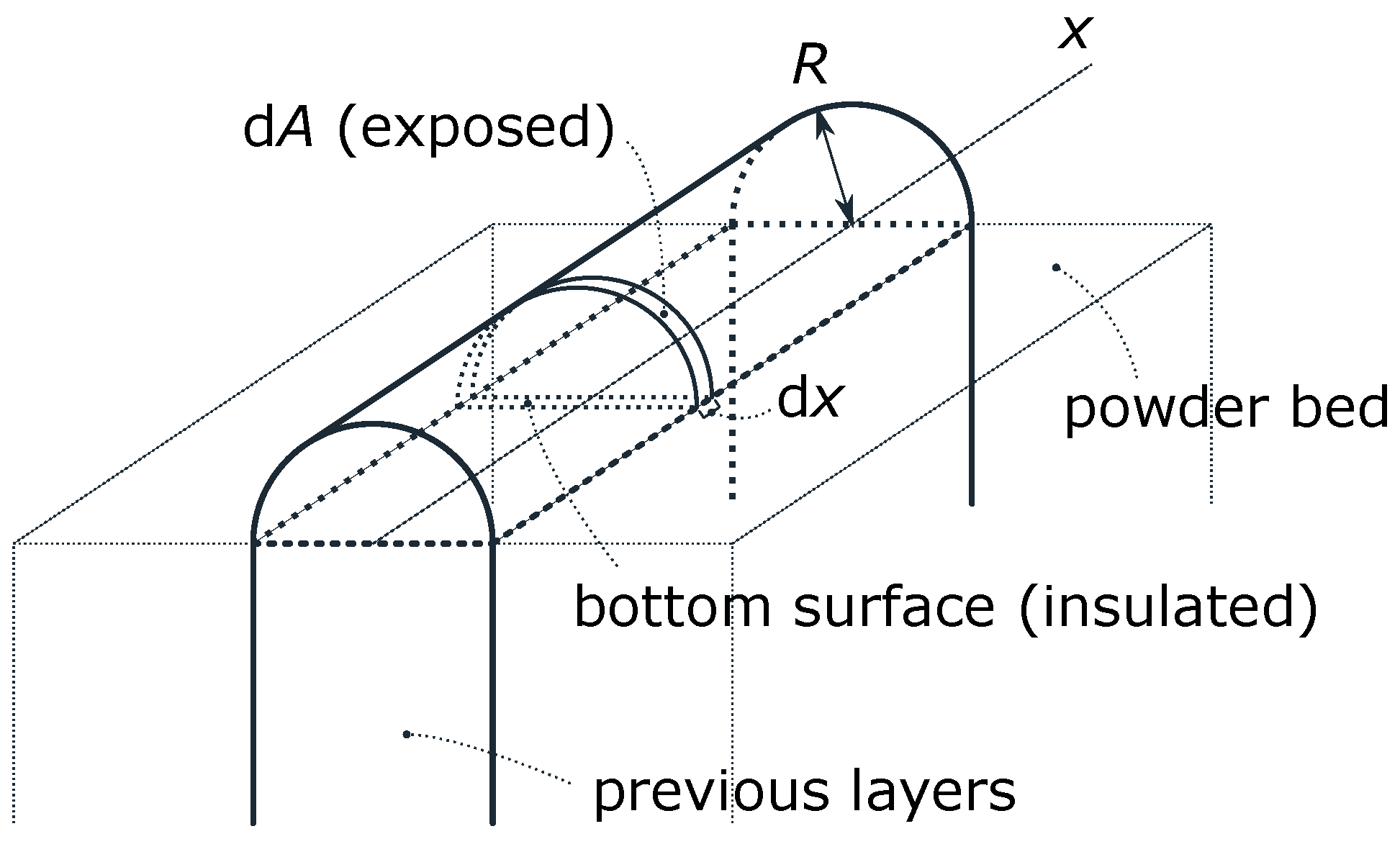
The SI unit of the heat source is , so the unit of r in (15) must be . However, a standard heat transfer coefficient, which we denote by , across a surface has the unit . To relate r to the standard format, as an example, let us consider the printed layer to have a semi-circular cross section with radius R, with the round part exposed to air.
The exposed surface area of a small but finite length of the semi-circular cross section in Figure 3, and the mass contained in the same length are, respectively,
In the ratio , which represents exposed surface area per unit mass, the cancels, so this ratio stays constant as we let :
Matching the units of r and , the heat transfer coefficients are related by
where for our example configuration is given by (18).
This example configuration underestimates the cooling, because the bottom surface that is in contact with the previous layer is treated as a perfect thermal insulator, and the powder bed is not accounted for. However, it is straightforward to modify the modeling assumptions. For example, given the appropriate standard heat transfer coefficients , it is possible to model a rectangular cross-section where the top is exposed to air, while the sides are in contact with the powder bed. The generalization of (19) to contact with multiple surfaces with different heat transfer coefficients (each at the same temperature ) is
where is the surface area (of length ) exposed to environment j, and as before, is the total surface area of the length , and is the mass contained in the length . For a surface that behaves as a thermal insulator, . Furthermore, to use a different temperature for each environment j, we may replace the cooling law (15) with a sum of such laws over the environments:
Thus, the only modification needed is to replace the term . For simplicity, in the following we use only one environment.
4. Nondimensional Equations for the Steady State
Let us now restrict our Eulerian description to the steady state, where . Inertial effects will remain in the form of the operator . To facilitate solution, we transform both (13) and (16) into a nondimensional form. Changing to nondimensional variables
we have
and
As is customary, we then drop the overbars from the notation. Each term of Equations (23) and (24) is dimensional, although the variables , and are nondimensional. We must normalize to bring the equations to a fully nondimensional form.
Normalizing Equation (23) by its highest-order coefficient leads to
Similarly, normalizing (24) by yields
Our problem has 11 dimensional parameters, namely , in 4 base units, namely . Therefore, by Buckingham’s theorem, there must exist exactly 7 independent nondimensional parameters. By solving for the null space of the dimension matrix, we find
Because the nondimensional parameters represent the null space of the dimension matrix, and the basis of a vector space can be chosen arbitrarily, the set of independent nondimensional parameters is not unique. We have chosen a basis that allows a physical interpretation for each parameter.
The independent nondimensional parameters through govern the fundamental physics of the system. In terms of the , the linear momentum balance (25) is expressed as
and the internal energy balance (26) becomes
The solution parameters P, and are not fully independent. In the thermal problem,
which is valid when . Furthermore, the thermal and mechanical solution parameters are coupled by
We will however keep the original in the energy balance equation to cover also the case ; keep in mind that does not depend on v, and in general, cannot be expressed in terms of the . However, if , then the parameterization is applicable, and .
Equations (34) and (35) form a unidirectionally coupled thermomechanical problem. We may first solve (35) for the temperature T, and then use that in (34) to determine the displacement u.
In a steady state, , so as a bonus, by rearranging (35), we obtain an expression for the material parcel cooling rate in the steady state (writing out the overbars for clarity):
which gives the dimensional cooling rate (unit ) as a function of the nondimensional temperature field .
5. Solution of the Thermal Problem
The solution of the second-order nonhomogeneous linear ordinary differential Equation (35) is the sum of a particular solution, which we may take to be , and the two linearly independent solutions of the corresponding homogeneous equation
By inserting and then factoring out the standard ansatz , the characteristic equation is
The roots of the characteristic equation are ()
where and are defined in (35). Provided that (i.e., , heat escapes via the exposed edge), the value is not a root. Therefore, both solutions are exponential functions; there is no solution as a linear function of x. Furthermore, since we always have , it follows (regardless of ) that the discriminant , so the two roots are always real, distinct, and nonzero. The roots merge only if both and (which leads, in the limit, to a double root at ).
Taking these considerations together, for , the nondimensional temperature field is
where are the roots of the characteristic polynomial, given by (41). Regardless of , we have and ; therefore, one of the exp saturates toward the right (for , cooling effect via the exposed surface) and one toward the left (for , heat escaping through the endpoint ).
For but (stationary material, ), the roots simplify to . The steady-state temperature profile can then be expressed as a linear combination of and . However, we prefer the general representation (42), because it can also deal with the asymmetry that is introduced when .
From (42), the nondimensional temperature gradient is
6. Solution of the Mechanical Problem
By defining the auxiliary variable
the linear momentum balance Equation (34) reduces to a linear first-order ordinary differential equation in w. It can be solved analytically (even with arbitrary function coefficients) using the standard formula; see, e.g., Kreyszig ([22] pp. 30–31). The nondimensional solution is
where is a constant of integration, to be determined from mechanical boundary conditions, and the effect of the external force on the solution is described by the function :
Inserting the thermal solution (42) and integrating (48) twice, the nondimensional displacement becomes
where and are constants of integration. The nondimensional solution parameters P and are defined in (34), and the thermomechanical coupling is represented by the parameters ()
where are the roots of the characteristic polynomial of the thermal problem.
For the mechanical problem, we take the boundary conditions
where , and are prescribed values. Thus, out of the parametric family of solutions of the mechanical problem, we pick the unique solution based on behavior at the inflow boundary only. In a sense, the outflow boundary is left free to develop.
However, this is very different from a free-of-traction boundary condition; we are not specifying any mechanical boundary condition at the outflow boundary. The displacement is described by a three-parameter family of functions, with three constants of integration ; we may use any three independent pieces of information to derive values for the constants. We are simply picking, out of all admissible solutions, the unique solution that, at the inflow boundary, has zero displacement, zero strain, and zero derivative of strain.
Using the expression (50) in (52), we obtain the following linear equation system for the constants of integration :
This system has a unique solution as long as and (so that the solution actually is (50)) and (so that the nondimensional solution parameter P is nonzero).
By Gaussian elimination, the constants of integration are given by
Keep in mind that these constants of integration are specific to the mechanical boundary conditions (52) and to the mechanical solution (50). Thus, if we wish to use different boundary conditions for the mechanical problem, we must derive new constants of integration accordingly.
Furthermore, to produce the mechanical solution (50), we have used our thermal solution, Equation (42). Therefore, the constants (54) relate not only to the mechanical part of the problem, but to the thermomechanical problem as a whole. However, we may change the boundary conditions of the thermal problem without affecting the result (54), because such modifications only change the expressions of and .
Inserting the constants (54) and the nondimensional parameters into (50), we obtain the nondimensional displacement . Converting back to dimensional variables, the dimensional displacement is . The strain is , where in the last step, the conversion factors cancel.
Finally, the stress is obtained from the constitutive law (8). Performing the replacements and , and using the fact that in a steady state, , the constitutive law becomes
7. Numerical Examples
In the following examples, we use parameter values for 316L steel, as listed in Table 1. The data for , , , c, and k is taken from [23]. The density and the coefficient of thermal expansion are reported as functions of temperature in Table 7 in the reference. Similarly, the specific heat capacity c can be found in Table 2 in the reference, and heat conductivity k in Table 10. Discussing the data for c, the author points out (in sec. II. A) that the tables are based on experimental data, but with smoothing, and with extrapolation to the melting range, reported as . Due to extrapolation, some caution may be needed, but the data quality is sufficient for the purposes of producing representative numerical examples. The distinction between solidus and liquidus temperatures is ignored, and a unique melting point is defined as . We also follow this choice.
The data for E is taken from ([24] table on p. 43, and Figure 27). The Young moduli of the different steel types discussed in the report are all close enough to use this data, measured for type 316, also for 316L steel.
We set as our reference temperature for nondimensionalization, . The temperature is also the reference temperature where we consider thermal expansion to be zero, so is a convenient reference temperature for our case where the metal solidifies and starts cooling.
As for the viscosity , steel in its solid phase is usually not considered a viscous material. Damping properties, especially for linear constitutive models, are in engineering sometimes given in terms of the loss factor (), which describes the damping of complex-valued harmonic vibrations as a function of the angular frequency (unit ).
Some of the damping comes from structural features of the experiment setup where the measurements are made, while some comes from the viscosity of the material being tested. We here consider all of the damping as coming from the viscosity of the material, thus leading to an upper limit for the viscosity.
The loss factor is defined as (see, e.g., Lewandowski and Chorazyczewski ([25] remark after Equation (9)))
where is the loss modulus (representing viscous dissipation), and is the storage modulus (representing the elastic response, which is fully recoverable). The loss factor is a nondimensional quantity. Specifically for the Kelvin–Voigt model, these moduli are related to E and by (see the review by Banks et al. ([26] p. 31))
where f is the vibration frequency in . Thus, the viscosity and Kelvin–Voigt retardation time are, respectively,
Sarlin et al. [27] have measured the loss factor of plain cold rolled steel sheets and bare stainless steel sheets in the frequency range from to . The ratio varies as varies, and it is not a monotonic function of . The minimum and maximum values of the ratio are obtained as and , respectively. Note that these differ by a factor of .
We use the representative value , motivated by both the results of Sarlin et al. [27], as well as the references therein. The vibration frequency is set to a representative value ; making the frequency as low as reasonable maximizes the estimated value of viscosity. Evaluating the Kelvin–Voigt retardation time yields the value given in Table 1, so that the viscosity of 316L steel becomes
The retardation time is on the order of , so even by this cautious estimate, steel in its solid phase is almost purely elastic (in the stress range below the plastic yield stress).
As for Newton’s law of cooling, the convective heat transfer coefficient across a solid-fluid interface into air varies significantly depending on the experiment conditions. For free convection, Kosky et al. ([28] Table 14.2) give the range , and for forced convection, . In our examples, we use a representative value of .
Taking for our semi-circular cross section to obtain a printing line width, and using our average density , the heat transfer coefficient per unit mass becomes, by Equation (19),
For the thermal problem, we take to represent material that has just solidified; and as was mentioned, thermal equilibrium at outflow, i.e., . The temperature is nondimensionalized by , so for the nondimensional temperature, .
As for the process parameters, we take there to be no external mechanical forces, . We take the length of the Eulerian domain as , and the frame velocity as . Thus, the material parcel travel time across the domain is . In reality, this is the laser travel time across the chosen length L; but in our Eulerian view, the laser remains stationary at , while the material parcels move through the domain.
Because our thermal boundary conditions specify thermal equilibrium at the outflow point, in order for the model to be valid, we must make large enough compared to , to allow sufficient cooling to occur for each material parcel before it hits the outflow boundary. With the parameter values given, we have , which is much larger than 1, as required.
The numerical examples are shown in Figure 4, Figure 5, Figure 6, Figure 7 and Figure 8. Computations have been performed using software-based arbitrary-precision floating point, because with the parameters used in the examples, some arguments to the exp function become so large that the result overflows the standard IEEE 754 double-precision floating point representation. Results can nevertheless be obtained in real time, because the number of calculations to evaluate the solution at one point is very small, and points per curve is sufficient to produce a visualization that looks smooth.
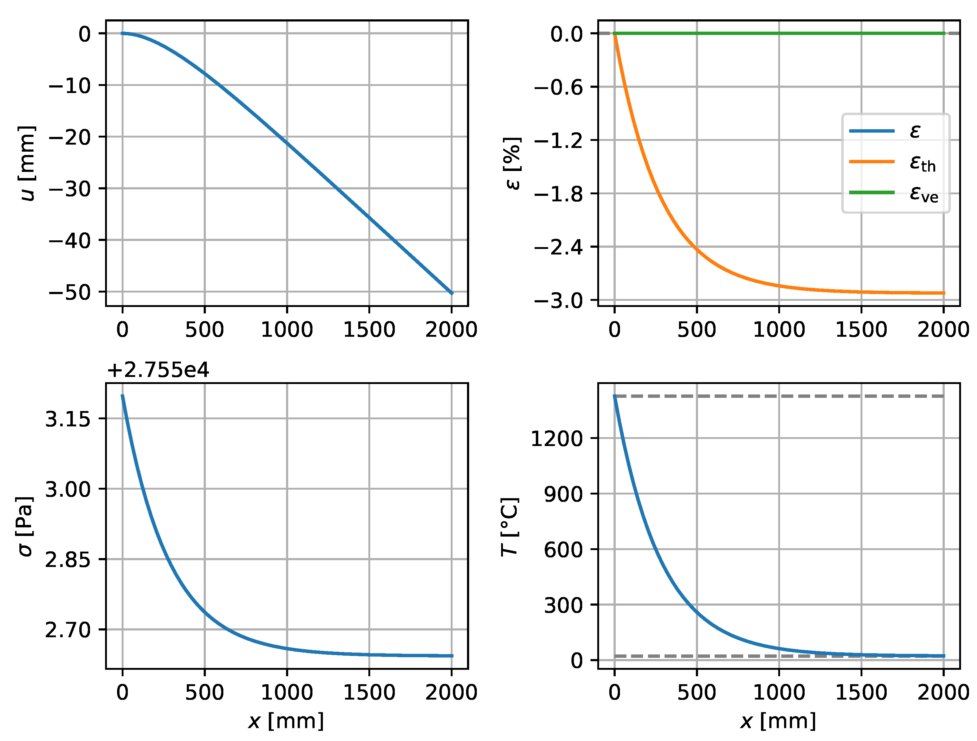
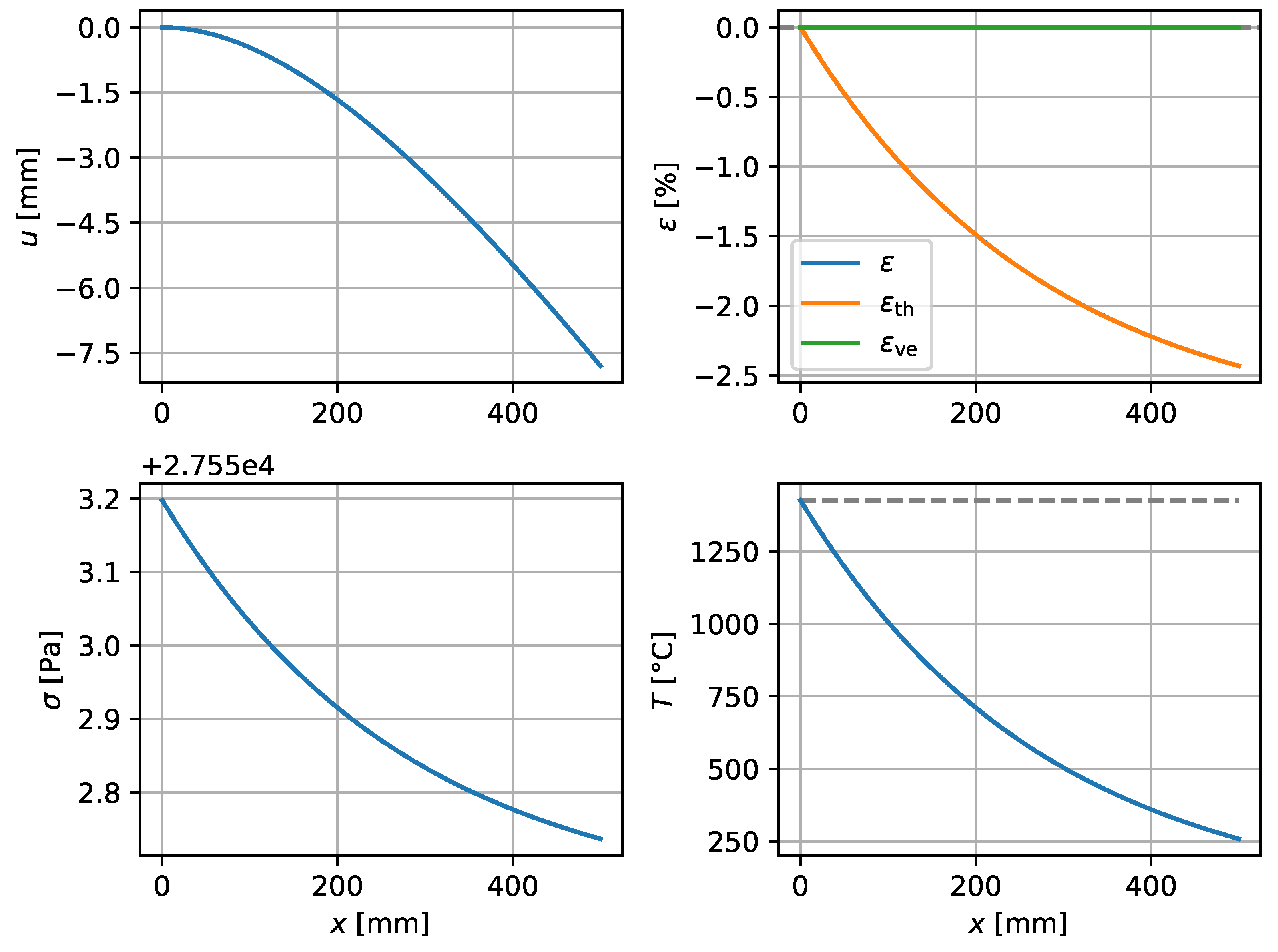
Figure 4 presents the results for 316L steel. As is seen in the figure, the total strain saturates at . Almost all of this is thermal shrinkage; the viscoelastic strain saturates at (note exponent). The viscoelastic strain is tensile, while the thermal and total strains are compressive. At the lower left subfigure displaying the stress, note the range of ; stress is generated only by the viscoelastic strain. The maximum stress is (positive, tensile) at , and the stress varies across the domain from this value by less than one pascal. In the lower right subfigure displaying the temperature, the upper marked temperature is the melting point at ; the lower marked temperature is the temperature of the environment at .
All mechanical boundary conditions are given at the inflow point at . The solution is valid for any shorter domain, simply by cutting the figures at the desired value of x. Figure 5 shows a zoomed detail of Figure 4 up to .
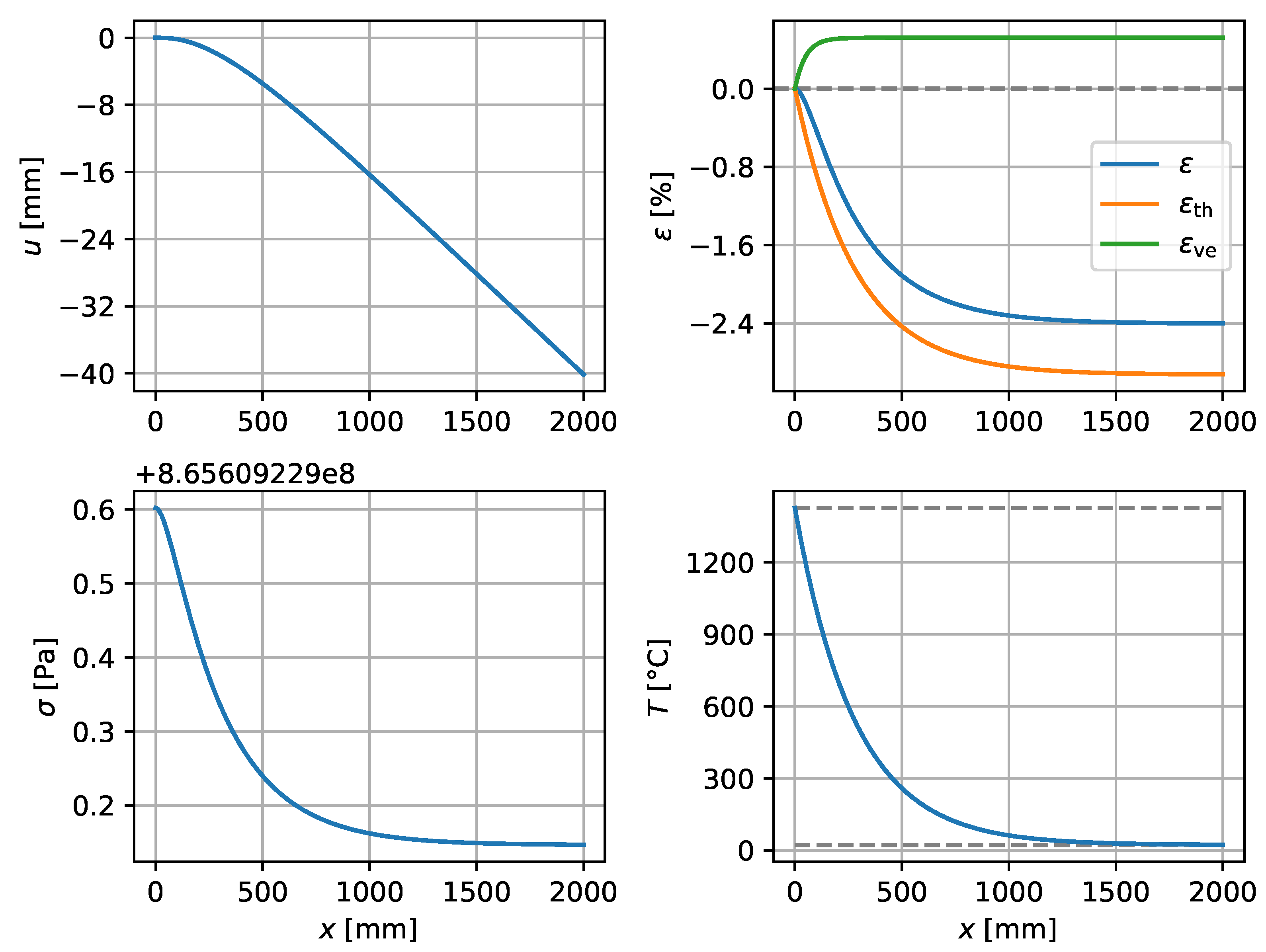
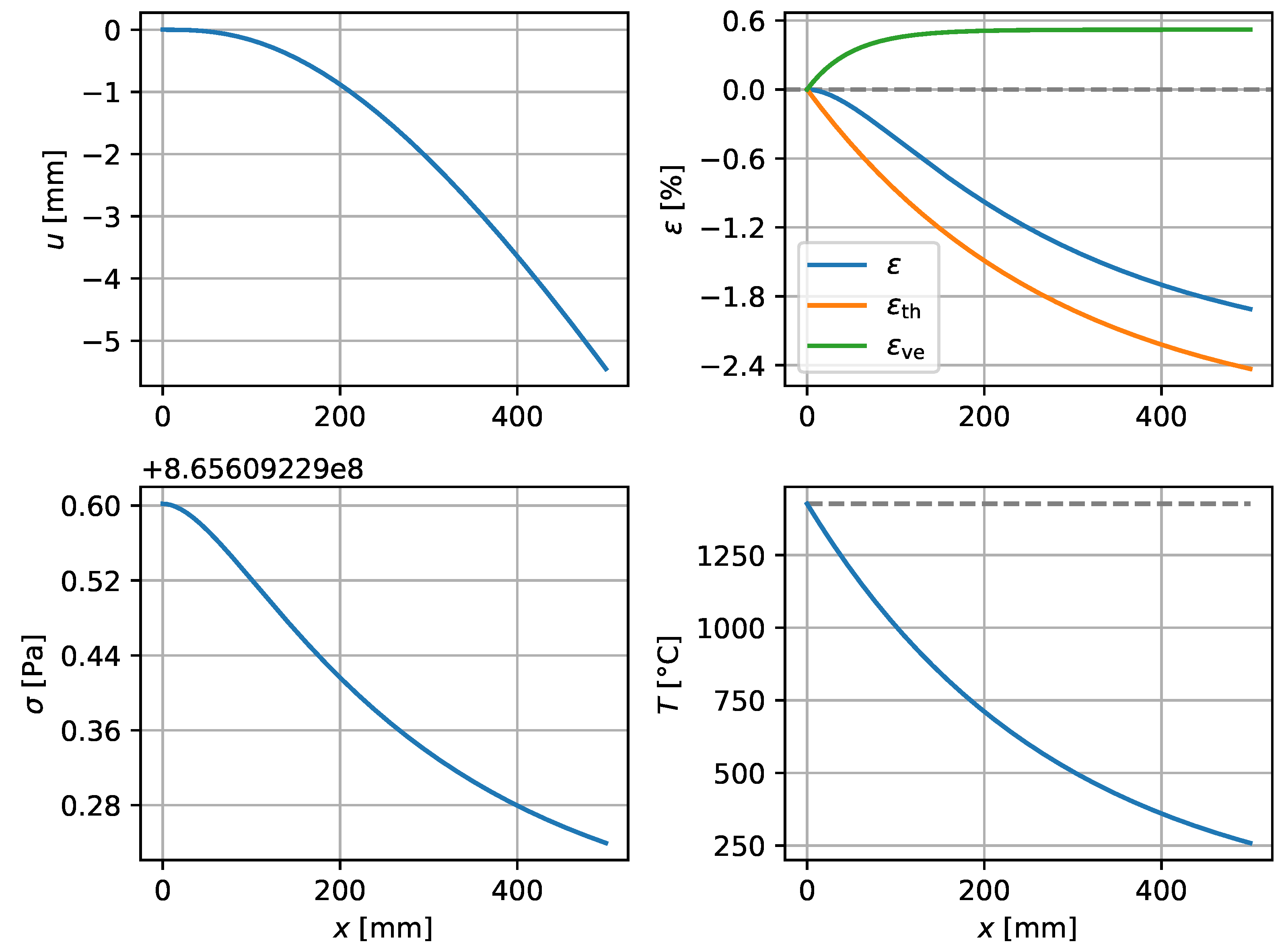
Figure 6 and Figure 7 similarly show the behavior of the model at an artificially high viscosity, for comparison. The material is otherwise exactly like 316L steel, but with viscosity significantly increased to have a Kelvin–Voigt retardation time of , which is approximately times higher than for steel. The temperature field remains the same as for 316L steel. Now the viscoelastic strains saturate at , , and . As before, the viscoelastic strain is tensile, while the thermal and total strains are compressive. The stress level is now high; , but the variation in the stress across the domain still remains at less than one pascal. This indicates that the almost constant stress predicted for 316L steel cannot be due to the short retardation time of the material.
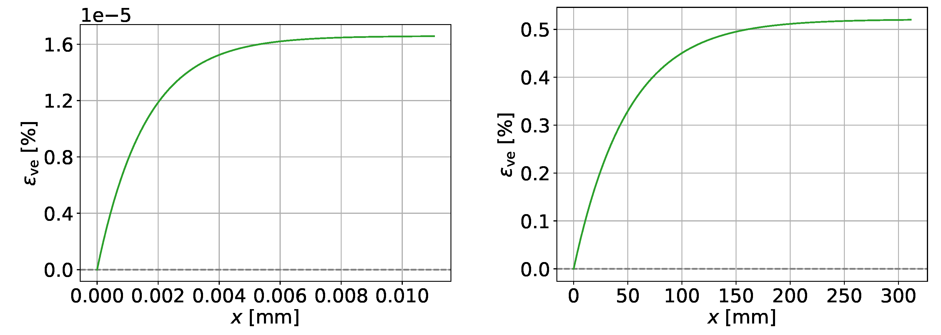
Figure 8 shows the viscoelastic strain, which causes the stress. With the parameters used in our examples, for 316L steel, the viscoelastic strain saturates at approximately (note scale), whereas in the artificially viscous example, saturation is reached at approximately . At , these correspond to a saturation time of and , respectively. These differ by a factor of 30,000, as expected for a Kelvin–Voigt material, given the ratio of the retardation times.
8. Conclusions
In this study, we considered the thermomechanical behavior of the laser-based powder bed fusion (L-PBF) additive manufacturing process during the printing of a layer of a vertical fin at constant velocity. Using an approach from analyses in process industry applications, we considered the laser as stationary and the material as moving, and applied an Eulerian perspective to the axially moving solid. With the goal of finding an analytical solution, we proceeded to construct a radically simplified one-dimensional thermomechanical model. Its parametric analytical solution was obtained.
The approach was applied from a theoretical perspective, to expose the fundamental behavior of the process. Expansion into more detailed computational and experimental studies was left open for later. This systematic approach allows the present study to act as a point of comparison, to clearly display which effects are introduced by each specific refinement of the model.
The main advantages of the analytical solution are the ease of implementation, and the speed at which the parameter space of the model can be explored. The main drawback compared to a more complex numerical simulation is the accuracy. Particularly, as Denlinger et al. [3] point out, heat conduction via the powder bed should be included in models of the L-PBF process in order to avoid overestimating the temperature. However, given the appropriate heat transfer coefficients and geometric modeling assumptions, the cooling model can be easily adjusted to account for this.
By a dimensional analysis, the seven nondimensional parameters that govern the fundamental physics of the considered system were obtained. These parameters allow generalization into multiple space dimensions, by performing an analogous nondimensionalization of the multidimensional tensor equations.
Even with more complex models, it is possible to produce a representative computational atlas of solutions in different regions of the nondimensional parameter space. Then, by mapping the physical parameters into nondimensional parameters, one may look up the solution in the pre-computed atlas that most closely corresponds to a given real-world application. This has applications in real-time control of the L-PBF process.
The material parameters were treated as constants independent of temperature mainly in order to produce an analytically solvable model. In the slightly more complex case where the material parameters are modeled as linear functions of temperature, in the absence of the cooling term, it is actually possible to derive an analytical solution for the internal energy balance. This results in a separable Abel equation of the second kind for the temperature field , for which an analytical solution exists as an explicit inverse function ; see Polyanin and Zaitsev ([29] p. 10, and Section 1.3.4). The integral that appears in the explicit solution can itself be explicitly solved using a partial fraction decomposition of the integrand. The function can be inverted numerically to obtain for the right-hand side when computing the displacement . With the appropriate transformations, the displacement is analytically solvable in terms of the temperature field. This results in a semi-analytical solution algorithm for the coupled problem. However, if the cooling term is added to this modified model, the internal energy balance no longer admits such a straightforward reduction to an analytically solvable form; hence this variant was not considered here.
For any model of the considered situation that is more complex than the one that was solved, a numerical solution strategy is recommended. When solving the governing equations numerically, it must be kept in mind that the linear momentum balance in the Eulerian formulation of a Kelvin–Voigt solid includes a third derivative, so when using finite elements, either continuous elements or a mixed-form strategy must be employed. This is also true for the next more complex material model, the standard linear solid (SLS).
Possible future directions include numerical studies in two and three space dimensions, more complex material models, and a more realistic cooling model. It will also be interesting to consider the contributions of the powder bed and the melt pool to the thermomechanical response of the printed object.
Author Contributions
Conceptualization, M.K.; Data curation, J.J. and M.K.; Formal analysis, J.J.; Funding acquisition, T.T. and M.K.; Investigation, J.J. and M.K.; Methodology, J.J. and M.K.; Project administration, T.T. and M.K.; Resources, M.K. and T.T.; Software, J.J.; Supervision, M.K.; Validation, J.J. and M.K.; Visualization, J.J.; Writing—original draft, J.J. and M.K.; Writing—review and editing, J.J., T.T. and M.K. All authors have read and agreed to the published version of the manuscript.
Funding
This research was funded by the European Regional Development Fund (projects Additive/A76103 and iADDVA/A77069).
Institutional Review Board Statement
Not applicable.
Informed Consent Statement
Not applicable.
Data Availability Statement
Not applicable.
Conflicts of Interest
The authors declare no conflict of interest. The funders had no role in the design of the study; in the collection, analyses, or interpretation of data; in the writing of the manuscript, or in the decision to publish the results.
References
- Milewski, J.O. Additive Manufacturing of Metals; Springer Series in Materials Science; Springer: New York, NY, USA, 2017; Volume 258. [Google Scholar] [CrossRef]
- Peng, X.; Kong, L.; Fuh, J.Y.H.; Wang, H. A review of post-processing technologies in additive manufacturing. J. Manuf. Mater. Process. 2021, 5, 38. [Google Scholar] [CrossRef]
- Denlinger, E.R.; Jagdale, V.; Srinivasan, G.V.; El-Wardany, T.; Michaleris, P. Thermal modeling of Inconel 718 processed with powder bed fusion and experimental validation using in situ measurements. Addit. Manuf. 2016, 11, 7–15. [Google Scholar] [CrossRef]
- de Moraes, D.A.; Czekanski, A. Parametric thermal FL analysis on the laser powder input and powder effective thermal conductivity during selective laser melting of SS304L. J. Manuf. Mater. Process. 2018, 2, 47. [Google Scholar] [CrossRef] [Green Version]
- de Moraes, D.A.; Czekanski, A. Thermal modeling of 304L stainless steel for selective laser melting: Laser power input evaluation. In Proceedings of the ASME 2017 International Mechanical Engineering Congress and Exposition, Tampa, FL, USA, 3–9 November 2017. [Google Scholar]
- Mirkoohi, E.; Ning, J.; Bocchini, P.; Fergani, O.; Chiang, K.; Liang, S.Y. Thermal modeling of temperature distribution in metal additive manufacturing considering effects of build layers, latent heat, and temperature-sensitivity of material properties. J. Manuf. Mater. Process. 2018, 2, 63. [Google Scholar] [CrossRef] [Green Version]
- Irwin, J.; Michaleris, P. A line heat input model for additive manufacturing. In Proceedings of the ASME 2015 International Manufacturing Science and Engineering Conference, Charlotte, NC, USA, 8–12 June 2015. [Google Scholar]
- Gusarov, A.V.; Kovalev, E.P. Model of thermal conductivity in powder beds. Phys. Rev. B 2009, 80, 024202. [Google Scholar] [CrossRef]
- Kahl, M.; Schramm, S.; Neumann, M.; Kroll, A. Identification of a spatio-temporal temperature model for laser metal deposition. Metals 2021, 11, 2050. [Google Scholar] [CrossRef]
- Kiran, A.; Hodek, J.; Vavřík, J.; Urbánek, M.; Džugan, J. Numerical simulation development and computational optimization for directed energy deposition additive manufacturing process. Materials 2020, 13, 2666. [Google Scholar] [CrossRef]
- Lu, X.; Cervera, M.; Chiumenti, M.; Lin, X. Residual stresses control in additive manufacturing. J. Manuf. Mater. Process. 2021, 5, 138. [Google Scholar] [CrossRef]
- Sotiriou, M.P.P.; Aristeidakis, J.S.S.; Tzini, M.-I.T.T.; Papadioti, I.; Haidemenopoulos, G.N.; Aravas, N. Microstructural and Thermomechanical Simulation of the Additive Manufacturing Process in 316L Austenitic Stainless Steel. Mater. Proc. 2021, 3, 20. [Google Scholar] [CrossRef]
- Mokhtari, M.; Pommier, P.; Balcaen, Y.; Alexis, J. Laser welding of AISI 316L stainless steel produced by additive manufacturing or by conventional processes. J. Manuf. Mater. Process. 2021, 5, 136. [Google Scholar] [CrossRef]
- Letenneur, M.; Kreitcberg, A.; Brailovski, V. Optimization of laser powder bed fusion processing using a combination of melt pool modeling and design of experiment approaches: Density control. J. Manuf. Mater. Process. 2019, 3, 21. [Google Scholar] [CrossRef] [Green Version]
- Kreitcberg, A.; Inaekyan, K.; Turenne, S.; Brailovski, V. Temperature- and time-dependent mechanical behavior of post-treated IN625 alloy processed by laser powder bed fusion. J. Manuf. Mater. Process. 2019, 3, 75. [Google Scholar] [CrossRef] [Green Version]
- Risso, J.M.; Huespe, A.E.; Cardona, A. Thermal stress evaluation in the steel continuous casting process. Int. J. Numer. Methods Eng. 2006, 65, 1355–1377. [Google Scholar] [CrossRef]
- Bugeda, G.; Cervera, M.; Lombera, G. Numerical prediction of temperature and density distributions in selective laser sintering processes. Rapid Prototyp. J. 1999, 5, 21–26. [Google Scholar] [CrossRef]
- Skutch, R. Über die Bewegung eines gespannten Fadens, weicher gezwungen ist durch zwei feste Punkte, mit einer constanten Geschwindigkeit zu gehen, und zwischen denselben in Transversal-Schwingungen von gerlinger Amplitude versetzt wird. Ann. Der Phys. Und Chem. 1897, 61, 190–195. [Google Scholar] [CrossRef] [Green Version]
- Salonen, E.-M.; Koivurova, H. Comments on non-linear formulations for travelling string and beam problems. J. Sound Vib. 1999, 225, 845–856. [Google Scholar]
- Banichuk, N.; Barsuk, A.; Jeronen, J.; Neittaanmäki, P.; Tuovinen, T. Stability of Axially Moving Materials; Solid Mechanics and Its Applications; Springer: Cham, Switzerland, 2020; Volume 259. [Google Scholar]
- Allen, M.B., III; Herrera, I.; Pinder, G.F. Numerical Modeling in Science and Engineering; John Wiley & Sons: New York, NY, USA, 1988; ISBN 0-471-80635-8. [Google Scholar]
- Kreyszig, E. Advanced Engineering Mathematics, 7th ed.; John Wiley & Sons: Hoboken, NJ, USA, 1993; ISBN 0-471-59989-1. [Google Scholar]
- Kim, C.S. Thermophysical Properties of Stainless Steels; Report ANL-75-55; Argonne National Laboratory: Argonne, IL, USA, 1975.
- Nickel Institute. High Temperature Characteristics of Stainless Steel; A Designers’ Handbook Series No 9004; Committee of Stainless Steel Producers, American Iron and Steel Institute: Durham, NC, USA, 2020. [Google Scholar]
- Lewandowski, R.; Chorazyczewski, B. Identification of the parameters of the Kelvin-Voigt and the Maxwell fractional models, used to modeling of viscoelastic dampers. Comput. Struct. 2010, 88, 1–17. [Google Scholar] [CrossRef]
- Banks, H.T.; Hu, S.; Kenz, Z.R. A Brief Review of Elasticity and Viscoelasticity for Solids. Adv. Appl. Math. Mech. 2011, 3, 1–51. [Google Scholar] [CrossRef] [Green Version]
- Sarlin, E.; Liu, Y.; Vippola, M.; Zogg, M.; Ermanni, P.; Vuorinen, J.; Lepistö, T. Vibration damping properties of steel/rubber/composite hybrid structures. Compos. Struct. 2012, 94, 3327–3335. [Google Scholar] [CrossRef]
- Kosky, P.; Balmer, R.; Keat, W.; Wise, G. Exploring Engineering: An Introduction to Engineering and Design, 5th ed.; Academic Press: Cambridge, MA, USA, 2020; ISBN 978-0-12-815073-3. [Google Scholar] [CrossRef]
- Polyanin, A.D.; Zaitsev, V.F. Handbook of Exact Solutions for Ordinary Differential Equations, 2nd ed.; Chapman & Hall/CRC Press: Boca Raton, FL, USA, 2003; ISBN 1-58488-297-2. [Google Scholar]
Figure 1.
3D printing of steel using laser-based powder bed fusion (Trumpf TruPrint 1000).

Figure 2.
Problem setup for printing one line of metal. (Left): In the frame, the laser scans toward the left, at a constant speed v, over a stationary material. The effects of the scan angle are ignored, approximating the scan as linear motion. (Right): The setup used in the analysis. In the frame, the material moves toward the right, at the same constant speed v, under a stationary laser. We consider a length L of the axially moving material, starting from the trailing edge of the melt pool, where the material has just solidified.

Figure 3.
Example configuration for the cooling model: printed layer with semi-circular cross section.
Figure 3.
Example configuration for the cooling model: printed layer with semi-circular cross section.

Figure 4.
316L steel, , .

Figure 5.
316L steel, up to . .

Figure 6.
Artificial high-viscosity example, . , .

Figure 7.
Artificial high-viscosity example, , up to . .

Figure 8.
Viscoelastic strain. Left: 316L steel; note scale. Right: Artificial high-viscosity example, .
Figure 8.
Viscoelastic strain. Left: 316L steel; note scale. Right: Artificial high-viscosity example, .


Table 1.
Material parameters of 316L steel, used in the numerical examples.
| Quantity | Symbol | Value | Unit | Notes |
|---|---|---|---|---|
| Melting point | 1700 | midpoint of melting range | ||
| Density | average, | |||
| Coefficient of thermal expansion | ” | |||
| Specific heat capacity | c | ” | ||
| Heat conductivity | k | ” | ||
| Young’s modulus | E | average, | ||
| Kelvin–Voigt retardation time | loss factor at | |||
| Heat transfer coefficient to air | free or forced convection |
Publisher’s Note: MDPI stays neutral with regard to jurisdictional claims in published maps and institutional affiliations. |
© 2022 by the authors. Licensee MDPI, Basel, Switzerland. This article is an open access article distributed under the terms and conditions of the Creative Commons Attribution (CC BY) license (https://creativecommons.org/licenses/by/4.0/).
Share and Cite
MDPI and ACS Style
Jeronen, J.; Tuovinen, T.; Kurki, M. One-Dimensional Thermomechanical Model for Additive Manufacturing Using Laser-Based Powder Bed Fusion. Computation 2022, 10, 83. https://0-doi-org.brum.beds.ac.uk/10.3390/computation10060083
AMA Style
Jeronen J, Tuovinen T, Kurki M. One-Dimensional Thermomechanical Model for Additive Manufacturing Using Laser-Based Powder Bed Fusion. Computation. 2022; 10(6):83. https://0-doi-org.brum.beds.ac.uk/10.3390/computation10060083
Chicago/Turabian StyleJeronen, Juha, Tero Tuovinen, and Matti Kurki. 2022. "One-Dimensional Thermomechanical Model for Additive Manufacturing Using Laser-Based Powder Bed Fusion" Computation 10, no. 6: 83. https://0-doi-org.brum.beds.ac.uk/10.3390/computation10060083
Note that from the first issue of 2016, this journal uses article numbers instead of page numbers. See further details here.