Article

Improved Unsupervised Learning Method for Material-Properties Identification Based on Mode Separation of Ultrasonic Guided Waves

1
Institute for Mathematics, Mechanics and Informatics, Kuban State University, Krasnodar 350040, Russia
2
School of Mathematics and Statistics, Qingdao University, Qingdao 266071, China
*
Author to whom correspondence should be addressed.
Submission received: 1 May 2022 / Revised: 28 May 2022 / Accepted: 6 June 2022 / Published: 8 June 2022

Abstract

:
Numerical methods, including machine-learning methods, are now actively used in applications related to elastic guided wave propagation phenomena. The method proposed in this study for material-properties characterization is based on an algorithm of the clustering of multivariate data series obtained as a result of the application of the matrix pencil method to the experimental data. In the developed technique, multi-objective optimization is employed to improve the accuracy of the identification of particular parameters. At the first stage, the computationally efficient method based on the calculation of the Fourier transform of Green’s matrix is employed iteratively and the obtained solution is used for filter construction with decreasing bandwidths providing nearly noise-free classified data (with mode separation). The filter provides data separation between all guided waves in a natural way, which is needed at the second stage, where a more laborious method based on the minimization of the slowness residuals is applied to the data. The method might be further employed for material properties identification in plates with thin coatings/interlayers, multi-layered anisotropic laminates, etc.

1. Introduction

Non-invasive characterization of material mechanical properties is vital for condition monitoring to control the quality of samples and to identify possible damage or structural degradation during their service periods [1]. Vibration-based techniques have proven their efficiency for the evaluation of the elastic properties of small-scale samples [2]. However, due to the “global” nature of these approaches, their applicability for the characterization of certain structural parts, especially in large-scale engineering assemblies, might be restrained. Meanwhile, methods relying on ultrasonic guided waves (UGWs) provide an appropriate compromise between “global” and “local” structural evaluation and thus might serve as a suitable basis for corresponding non-destructive testing and structural health-monitoring applications [3,4,5,6,7,8,9]. UGWs are multi-modal waves and using them for material-properties identification often requires laborious signal processing. On the other hand, the benefit of the multi-modal nature is the availability of information on the wave characteristics in a wide frequency range, which improves the identification procedure. For instance, Cui and Lanza di Scalea [10] applied the advanced simulated annealing optimization algorithm to match pseudo-experimental phase velocity curves for fundamental modes (S0, A0, SH0) to computed velocity curves with varying constants in anisotropic laminate. It was shown in [11], where the fuzzy-based inversion technique was applied to the identification problem, that the inclusion of all UGWs better consolidates the identified uncertainties of the material properties compared to single-mode analysis in a broader frequency range. For identification algorithms, the UGWs’ separation is necessary, which is still challenging, since the dispersion effect leads to modal amplitudes of different levels and overlapping of the wave packages in the time-frequency domains. A significant number of researchers use the frequency–wavenumber representation, where the energy distributions of individual modes are naturally separated from each other. There are examples of the successful application of the matrix pencil method (MPM) and estimation of signal parameters via rotational invariance techniques (ESPRIT) based on the eigenvalue decomposition, such as singular value decomposition (SVD) [12,13,14]. Unfortunately, the number of modes is often not easily determined from thresholds using only eigenvalue intensities or singular values, and Okumura et al. [15] proposed an algorithm applying information-theoretic criteria efficient for SVD and ESPRIT methods. In [16], to obtain a time-frequency representation, an inverse synchronized wavelet transform was used, which makes it possible to automatically select individual modes after image processing. A time-frequency method of multi-modal dispatcher dispersion was also proposed for mode separation by Xu et al. [17]. However, the problem of automatic UGW separation has not been fully solved at the moment.
Machine-learning methods are now actively used in UGW propagation problems such as the mode separation related to unsupervised and self-supervised methods. For instance, Gaussian processes trained for different realizations of uncertain parameters were used for predicting the wave propagation with a convolutional neural network (CNN) to produce high-quality images of the wave patterns for new realizations of the uncertainty [18]. Non-negative matrix factorization was employed for mode separation with a subsequent classic clustering algorithm (DBSCAN) [19]. CNN were applied for the automatic selection of dispersion curves for the fundamental and higher modes of the 2D seismic profile [20], while a deep neural network (DNN) was trained to reconstruct plane wave ultrasound images from an RF channel [21]. The clustering of a series of data-points algorithms based on the feature extraction from multi-dimensional data was used for estimating complex frequencies and amplitudes of signals [14]. For machine-learning algorithms related to the identification of waveguide parameters, supervised learning methods have been also used recently, for instance, in [9,22,23,24], where the learning took place on synthetic data.
The principle of the method discussed in the current paper is based on the algorithm of the clustering of multivariate data series obtained as a result of the application of the MPM to the experimental data. In the proposed technique, multi-objective optimization is employed, which is usually used to improve the accuracy of particular-parameter identification [25]. At the first stage, the computationally efficient method based on the calculation of the Fourier transform of Green’s matrix (GMM) is employed (see [26] and references therein) iteratively, and the obtained solution is used for the filter construction with a decreasing bandwidth, which allows us to obtain nearly noise-free classified data (with mode separation). The filter provides data separation between all UGWs in a natural way, which is needed at the second stage, where a slower method based on the minimization of the slowness residuals (SRM) is applied to the data. The second step is important, since the SRM is more accurate than the GMM. On the other hand, the first step is indispensable to providing the mode separation needed for the SRM. Thus, the improved unsupervised learning method presented here is a multi-stage algorithm employing SRM at the second stage. Since SRM has the best convergence, the proposed method provides the same accuracy with lower computational costs reduced at the first stage, where the fast GMM is applied.

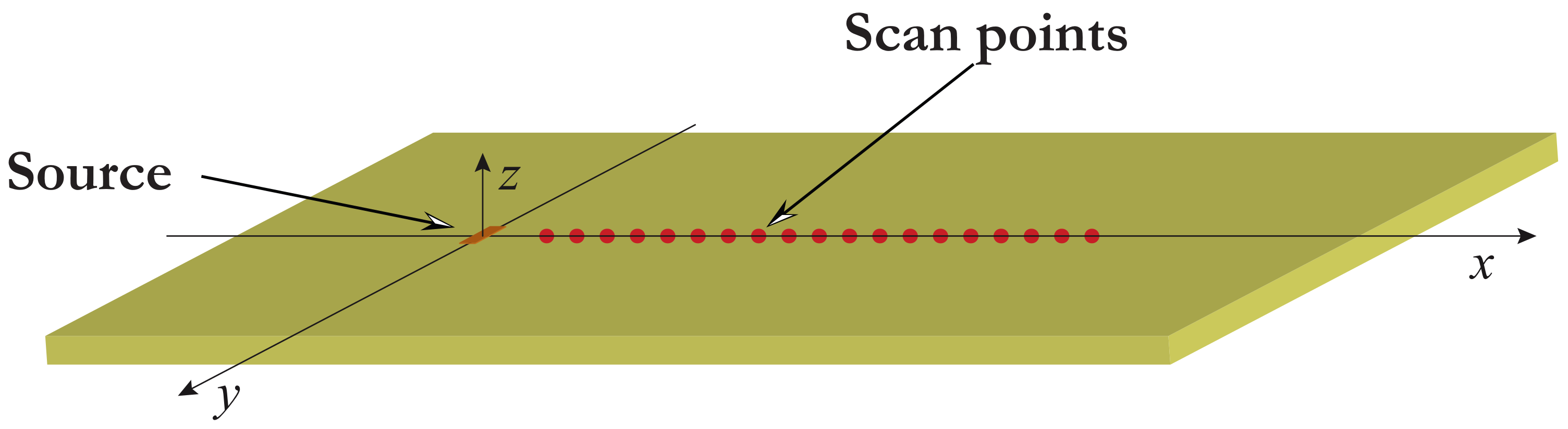
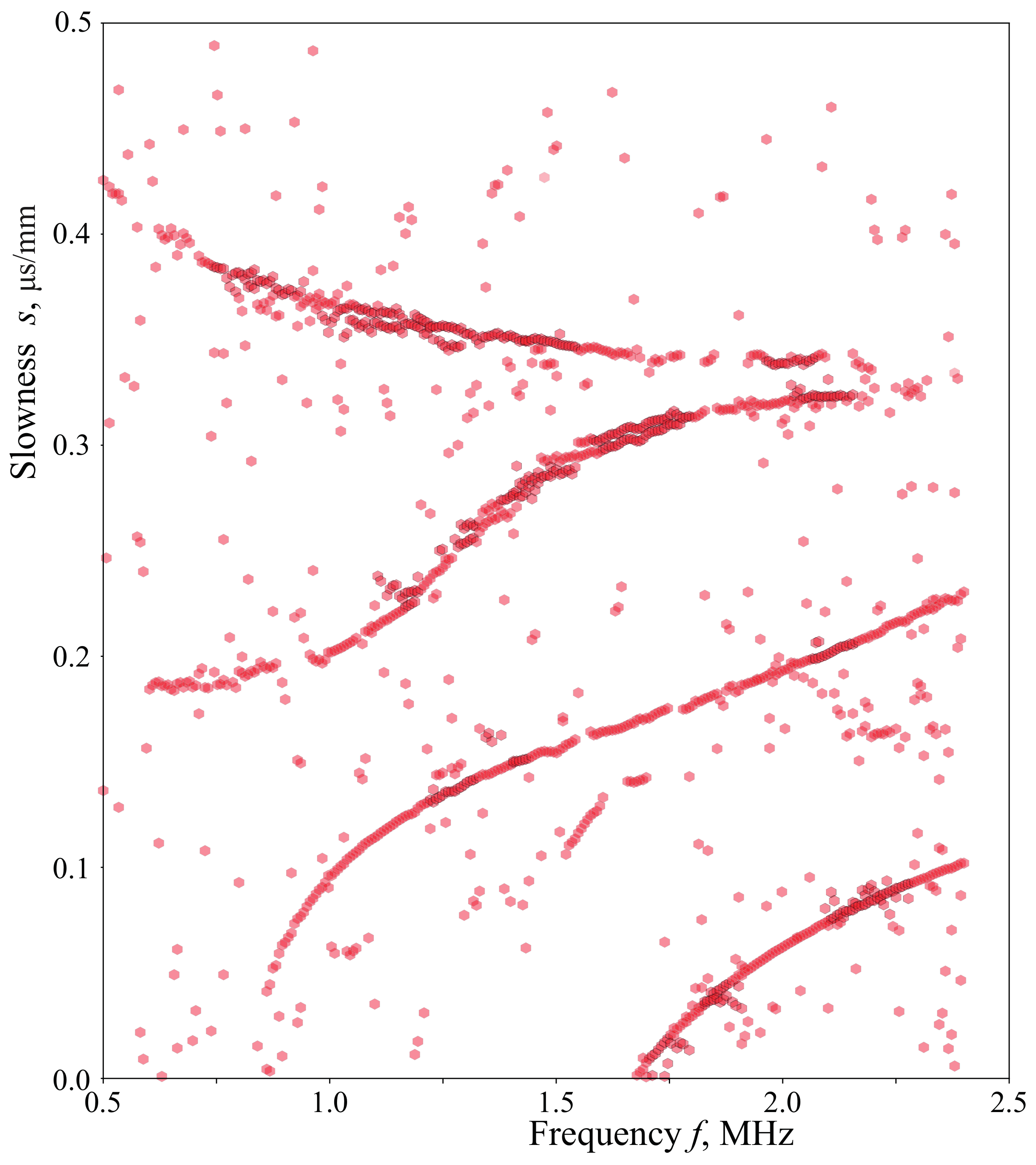
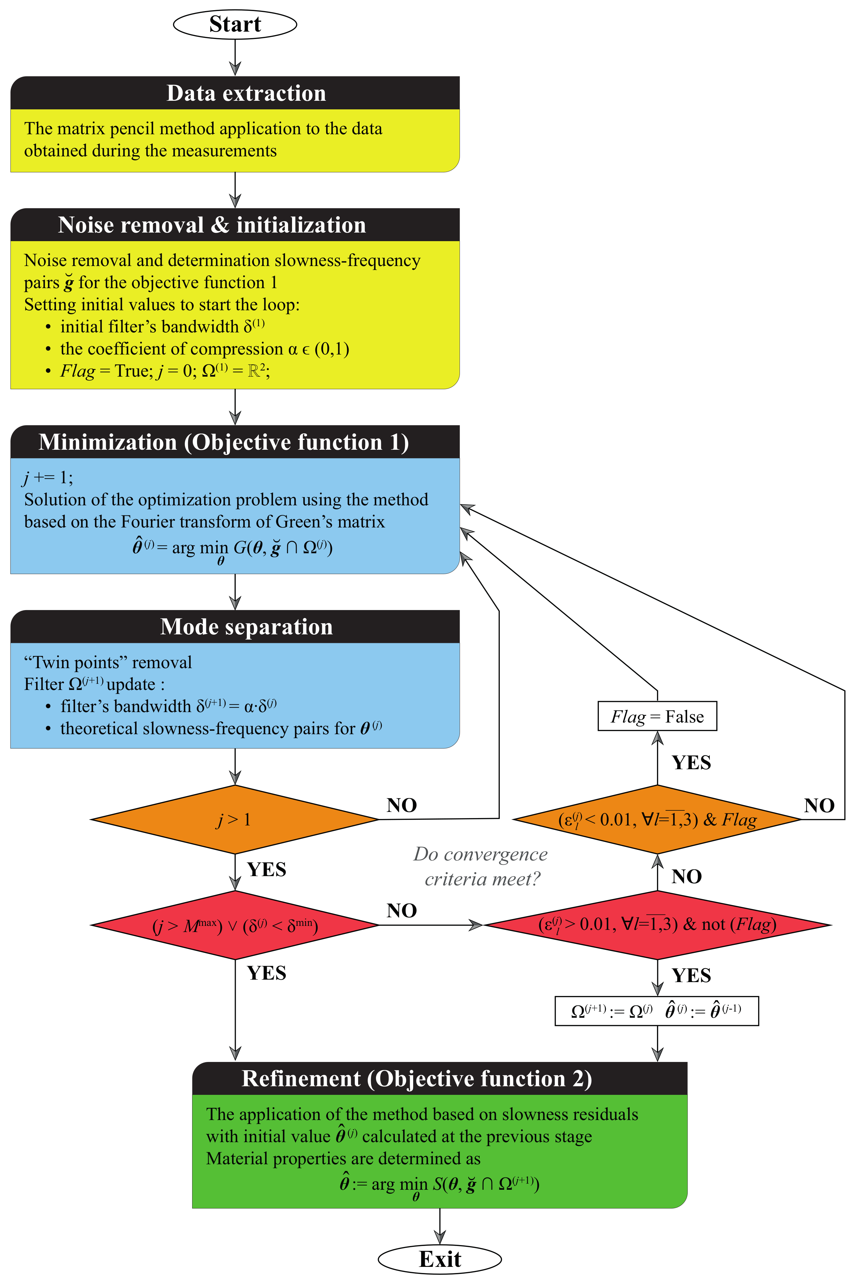
2. Data Extraction and Initialization

Various scanning techniques (laser Doppler vibrometry, phased arrays, air-coupled transducers) can be applied to obtaining data in the form of B-scans, which is necessary for data extraction in the first step. Let us consider an elastic plate, where the Cartesian coordinates are introduced so that the scan line goes along the O x axis, and the source exciting GWs is situated at the origin (Figure 1). Further on, it is assumed that the laser Doppler vibrometry is employed as a method for data acquisition at the surface z = 0 of the specimen, since it provides minimal distortion to the measured wavesignals [27] (out-of-plane velocities or displacements).
It should be noted here that the method of data acquisition at the surface z = 0 of the specimen (out-of-plane velocities or displacements) is not important for the proposed method (see Figure 1). Let us assume that velocities or displacements, denoted for simplicity as v ( x , 0 , 0 , t ) , are measured at N p points ( x i = x 0 + i Δ x , 0 , 0 ) at the moments of time t k = t 0 + k Δ t , and v ( x i , t k ) = v i k . These data is further processed with the MPM method, which allows to determine the relation between the wavenumbers k of propagating and evanescent guided waves and the frequency f. According to the MPM, the Fourier transform is applied to v ( x i , t k ) with respect to the time variable for a certain set of frequencies f n , n = 1 , N f ¯ , which gives V ( x i , f n ) = V i n .
Thus, for a certain frequency f n and a given set of scan points x i , the following approximation is to be constructed:
V i n m = 1 M A m n z m n i 1 = m = 1 M A m n e i k m n Δ x ( i 1 ) ,
where Δ x is the spatial step in the line scan, A m n are amplitudes related to poles z m n , which correspond to guided waves with wavenumbers k m n propagating at frequency f n .
Therefore, for the n-th frequency f n from a certain set of frequencies, the matrix pencil of two Hankel matrices X and Y are composed from the values V i n . Employing the singular value decomposition, for X = U · Λ · V , where U and V are unitary matrices and Λ ˜ = diag ( λ 1 , ) is a rectangular diagonal matrix. Then, the eigenvalues of the matrix pencil ( X , Y ) are determined using the reduced singular value decomposition of matrix X = U ˜ · Λ ˜ · V ˜ , which is obtained via the reduction of the first largest M singular values in Λ , i.e., Λ ˜ = diag ( λ 1 , , λ M ) , and U ˜ and V ˜ are corresponding unitary matrices. Therefore, the problem can be reduced to the eigenvalue problem for
U ˜ · X · V ˜ z Λ ˜
with respect to z values, which gives values of k n j . It should be mentioned that the number of poles M can be chosen specifically for each frequency.
The experimental setup described in detail in [28,29] was employed to gain experimental data in this study. Moreover, 3 MHz low-pass filtering was introduced with LDV software and a 7.8125 MHz sampling frequency was chosen to meet the Nyquist criterion. The LDV measurements were performed with Δ t = 10 7 s, Δ x = 0.25 mm, and N p = 200 . An example of the MPM application to determine the dispersion properties of an aluminium plate of 2 mm thickness is depicted in Figure 2, where slownesses s n m = k n m / f n were calculated for N f = 250 frequencies f n [ 0.5 , 2.4 ] MHz.
Thus, the MPM described in this section is applied at the first step to extract slowness–frequency pairs g ˘ = ( s ˘ n m , f n ) , m = 1 , M ¯ from the raw experimental signals (the parameter M of the MPM should be chosen with an assurance that it is larger than the number of propagating guided waves). Unfortunately, the data is usually noisy, and certain noise removal is needed.
The amplitudes A m n obtained after decomposition (1) are normalized for each frequency:
A m n : = A m n / max m ( A m n ) , n = 1 , N f ¯ .
Here, N f is the total number of frequencies f n in the set g . Further, the points with amplitudes A m n < 0.1 are removed from the dataset to clean up the noise. It should be noted that the increase in this threshold of 0.1 leads not only to the removal of the noise but also deletes the points belonging to the dispersion curves themselves (it could lead to the full disappearance of some modes that have not been intensively excited in the experiment). Such a noise removal gives the set of slowness–frequency pairs
g ˘ : = { ( s n m , f n ) , m B n , n = 1 , N f ¯ } ,
where the fact that the number of pairs varies from frequency to frequency is taken into account via the introduction of sets B n = { m | A ˘ n m > 0.1 } .

3. Objective Functions

3.1. Method Based on the Calculation of the Fourier Transform of Green’s Matrix

At the first stage of the proposed identification procedure, the GMM avoiding time-consuming root search procedures is applied. In the GMM, the minimization of the objective function G ( θ , g ) is performed so that the estimate is determined as follows:
θ ^ = arg min θ Θ G ( θ , g ˘ ) .
Here, θ is the vector of the parameters of the model and Θ denotes the bounds of the model parameters. The correctness was controlled using the bounds Θ = { 0.1 GPa < E < 300 GPa, 0.05 < ν < 0.499 , H > 0 } . The objective function G ( θ , g ˘ ) for the GMM is defined via the replacement of frequency f and slowness s into the inversion of the Fourier transform of Green’s matrix component K 33 1 ( f , s , 0 , θ ) :
G ( θ , g ) = 1 N n = 1 N f m B n min | K 33 1 ( f n , s ˘ n m , 0 , θ ) | , 1 ,
N = n = 1 N f | B n | .
An upper limit is introduced to avoid large values of objective function (2), which improves the effectiveness of the inversion procedure, since extremely large values could strongly influence the objective function [26]. For the examples considered in this study, the Fourier transform of Green’s matrix of an elastic homogeneous layer was used, but the proposed identification approach is also applicable for other kinds of waveguides.
Let us briefly describe the scheme of Green’s matrix composition in the case of a homogeneous stress-free elastic layer V = { | x | < , H z 0 } of thickness H with the mass density ρ , Young’s modulus E and Poisson’s ratio ν (see Figure 1). At least one parameter must be already determined for identification; otherwise, the solution is not unique. For the steady-state motion with the angular frequency ω = 2 π f , the displacement vector u in an elastic homogeneous isotropic media satisfies the governing equations:
1 ν 1 2 ν · u 1 2 × × u + ( 1 + ν ) ρ E ω 2 u = 0 .
The stress-free boundary conditions (Hooke’s law relates the components of the displacement vector u and the stress tensor σ i k ) are assumed at the surfaces of the waveguide
σ i 2 ( x , 0 ) = σ i 2 ( x , H ) = 0 , x .
The application of the Fourier transform to governing Equation (3) with respect to x 1 and boundary conditions (4) leads to the system of ordinary differential equations, where the unit vector is given on the right-hand side. The solution of the obtained system allows calculating the Fourier transform of Green’s matrix (see [30] for more details).

3.2. Method Based on the Slowness Residuals

In the second approach, the minimization of the residuals between measured slownesses s ˘ n m and theoretical slownesses s n m ( θ , f n ) is calculated employing the mathematical model (e.g., described in Section 3.1) with parameter θ at given frequency f n , see [26] for more details. To calculate the objective function
S ( θ , g ) = 1 N n = 1 N f m B n | s ˘ n m s n m ( θ , f n ) | ,
an accurate procedure for the mode separation is needed, since the distance between the theoretical and experimental slownesses corresponding to the same certain guided wave should be compared. Another disadvantage of the use of typical for objective function (5) is related to the numerical search of the roots of the dispersion equation, which are obtained via the application of the Fourier transform with respect to x 1 to governing Equation (3) and boundary conditions (4) for each frequency f n . The latter makes solution of the optimization problem
θ ^ = arg min θ Θ S ( θ , g ˘ )
computationally expensive.

4. Multi-Stage Algorithm for Material-Properties Characterization

The method proposed here is a combination of two approaches for material-properties identification, for which convergence and accuracy was demonstrated and analysed in [26]. The method based on the slowness residuals (SRM) is time-consuming, since it needs multiple calls for mode separation and search-root procedures. The computational time for the second method based on the calculation of the Fourier transform of Green’s matrix (GMM) is a hundred times smaller than for the SRM, whereas the computational time for one GMM call with 200 frequencies is ≈9 s on a laptop with Intel Core i3. The accuracy of the SRM is better (the GMM usually overestimates parameter values). All the stages of the proposed algorithm for waveguide-properties identification are briefly described in the flowchart shown in Figure 3, whereas a detailed description of the stages can be found in Section 2 and Section 3.
Step 1. In the first step, extraction of the information on dispersion characteristics of an inspected waveguide is performed. To this end, the MPM is applied to the experimental signal and some noise is removed, as described in Section 2. Before starting the loop at the next step, the bandwidth of filter δ ( 1 ) , the coefficient of filter bandwidth compression α ( 0 , 1 ) and bounds Θ , where the solution is allowed, are chosen. In addition, initial values Ω ( 1 ) = R 2 , g ˘ ( 1 ) = g ˘ and j = 0 , necessary for the first stage of the identification procedure, are determined at this step.
Step 2. An iterative procedure is repeated at the second step until the convergence criteria described further are met. According to the GMM, the solution of the optimization problem
θ ^ ( j ) = arg min θ Θ G ( θ , g ˘ ( j ) )
is obtained at the j-th iteration using the Broyden–Fletcher–Goldfarb–Shanno (BFGS) method. Here, Ω ( j ) describes the action of the filter
g ˘ ( j + 1 ) = g ˘ Ω ( j + 1 )
extracting from g ˘ only the pairs laying in the δ ( j ) vicinity of the theoretical slowness curves, i.e.,
Ω ( j + 1 ) ) = ( s , f ) | s ( θ ^ ( j ) , f ) δ ( j ) s s ( θ ^ ( j ) , f ) + δ ( j ) .
The bandwidth of the filter decreases at each iteration:
δ ( j + 1 ) = α · δ ( j ) .
The process is repeated at least two times. At the first iteration, no criteria are checked; then, relative error
ε l ( j ) = θ ^ l ( j ) θ ^ l ( j 1 ) θ ^ l ( j )
is considered to break the loop. A two-step criteria is proposed, and logical variable Flag (initial value is Flag = True) is used in the flowchart to explain the algorithm. Starting from the second loop, the condition ε l ( j ) < 0.01 is checked, and as soon it is satisfied, the logical variable changes it value (Flag = False). This condition is demanded to assure that the search becomes stable. The second condition is checked only if the first one is satisfied. The condition examines whether the search procedure is still stable and if the condition ε l ( j ) < 0.01 is not satisfied anymore, the loop is finished at the j-th iteration setting θ ^ l ( j ) : = θ ^ l ( j 1 ) and Ω ( j + 1 ) ) : = Ω ( j ) ) . Of course, the criteria related to the largest number of iterations ( j > M max ) and the minimum bandwidth of the filter ( δ ( j ) < δ min ) are also checked before continuing each loop for j > 2 .
Step 3. The converged solution θ ^ l ( j ) obtained at Step 2 applying the GMM in (6) is subsequently refined at the last step using the SRM method:
θ ^ = arg min θ Θ S ( θ , g ˘ ( j ) ) .
Since filter Ω ( j + 1 ) ) separates modes, a number of guided waves are easily distinguished in the SRM. To obtain better estimates, the optimization can be run several times using θ ^ ( j ) with a random additive less than 1% as an initial value for the minimization procedure. In this case, mean or median can be chosen to obtain a statistically accurate estimate for the material properties.

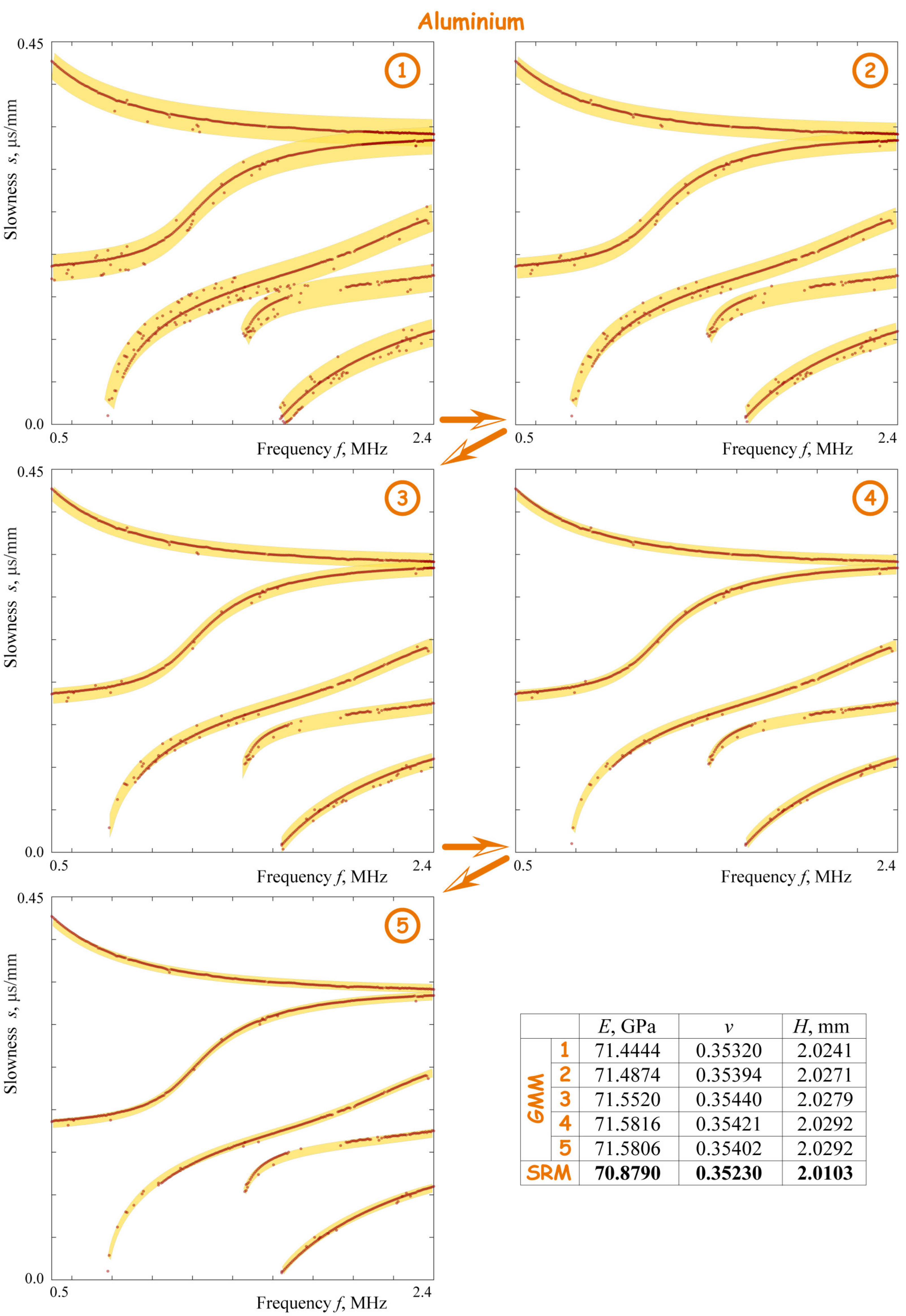
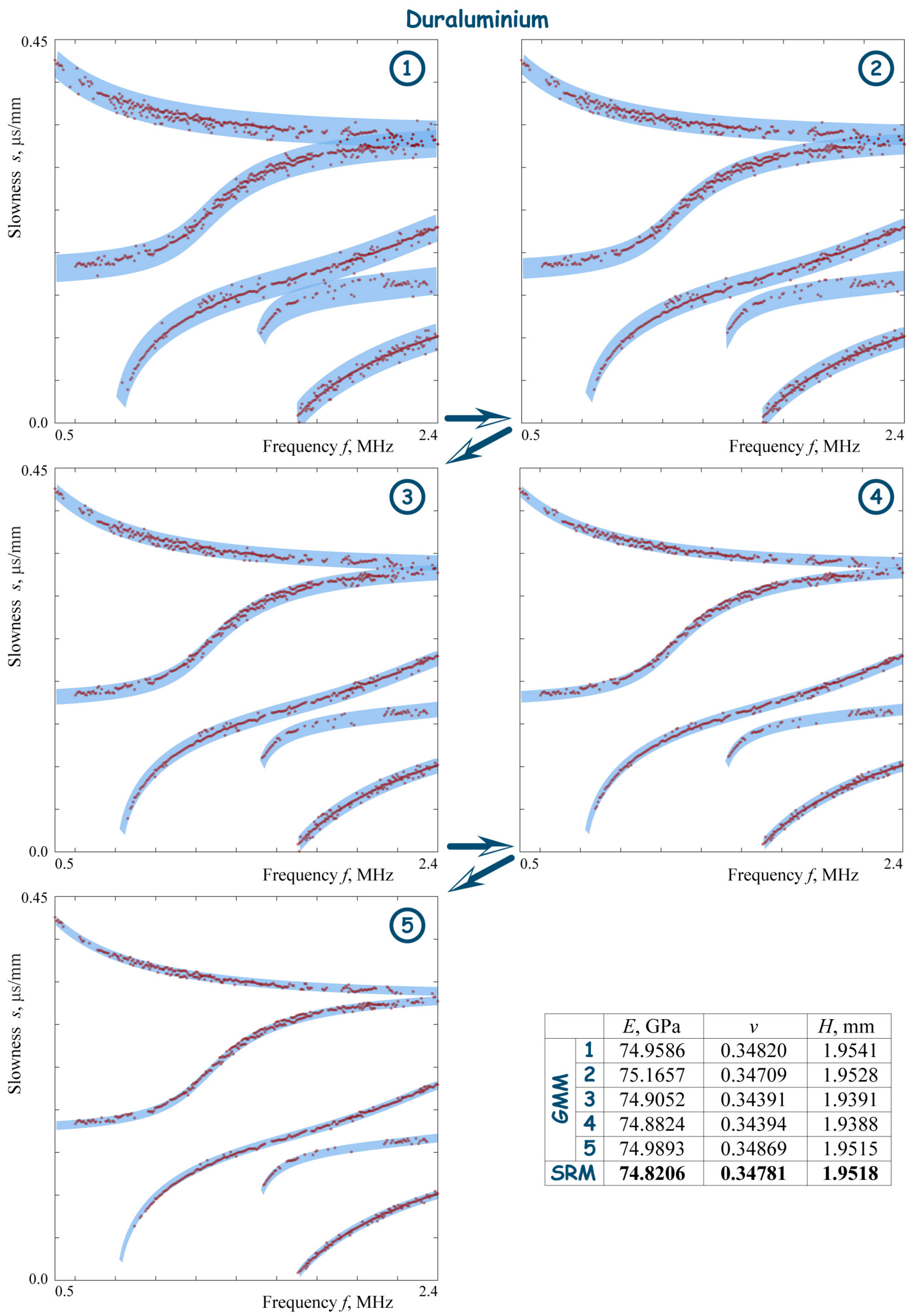
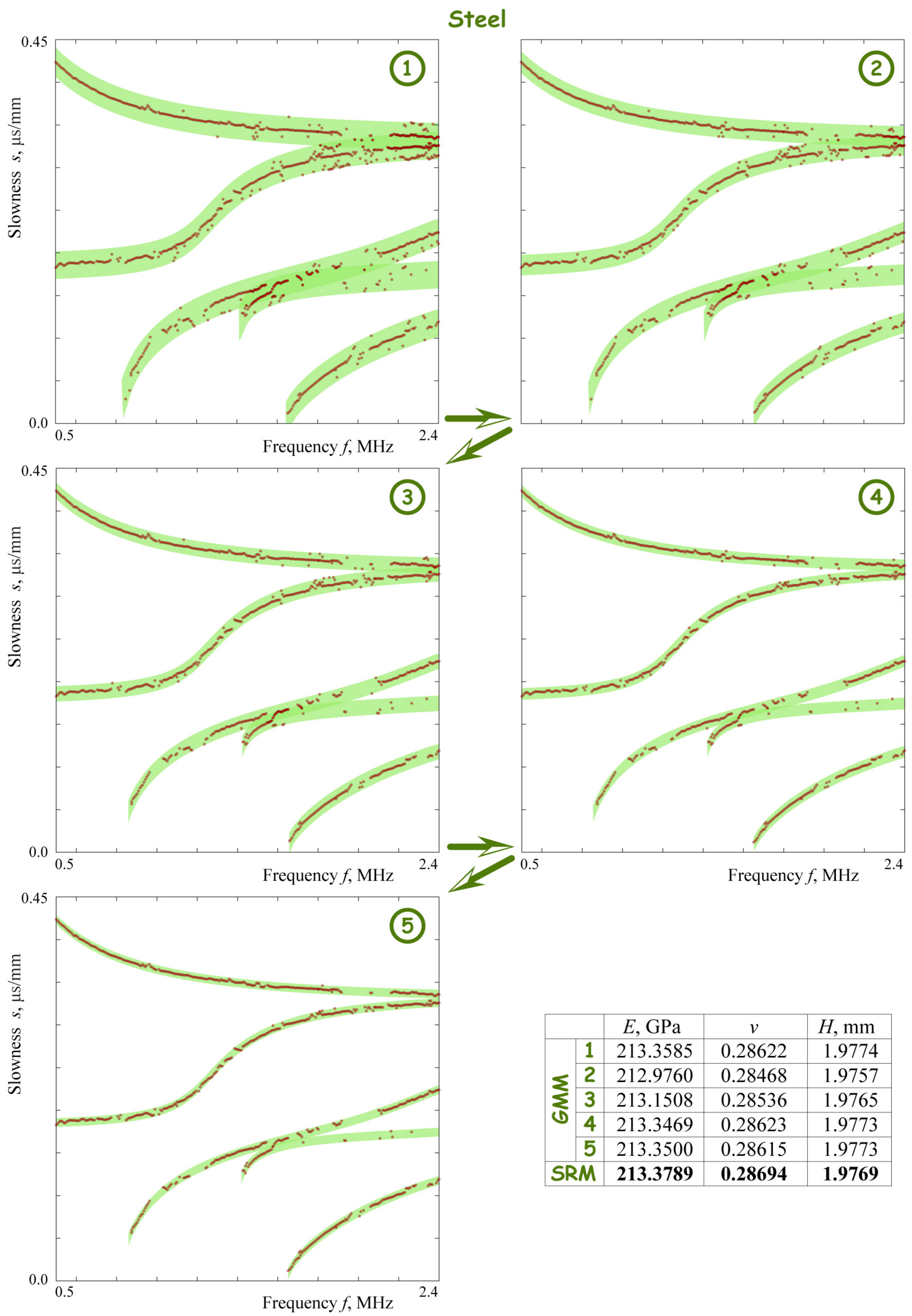
5. Examples of Material-Properties Identification Using Experimental Data

The proposed algorithm was verified and tested using experimental data measured for three different plates. Their thickness H and elastic properties, i.e., Young’s modulus and Poisson’s ratio, are unknown while density ρ is assumed to be known in advance. Ultrasonic GWs were excited in rectangular plates made of aluminium ( ρ = 2660 kg/m 3 and H = 2 mm), duralumin ( ρ = 2721 kg/m 3 and H = 1.9 mm) and steel ( ρ = 7843 kg/m 3 and H = 1.975 mm) by a circular piezoelectric actuator of a 5 mm radius and 0.5 mm thickness manufactured from PZT PIC 151 (PI Ceramic GmbH, Lederhose, Germany Germany). The out-of-plane velocities of propagating wave packages were measured at the surface of the specimen by PSV-500-V laser Doppler vibrometer (Polytec GmbH, Waldbronn, Germany) [31]. The actuator was driven by a broadband 0.5 μ s rectangular pulse tone burst voltage whose spectrum is non-zero for frequencies up to 3 MHz. It should be mentioned that material properties might be different at different temperatures [32], so the experimental data allows to identify the material properties of the specimen at the given temperature. In this study, the measurements were performed at 24 ° C.
Figure 4, Figure 5 and Figure 6 exhibit experimental slownesses g ˘ ( j ) filtered during the iterative process of Step 2 for the three considered plates with the known mass density. All the five iterations of the first stage of the improved algorithm are illustrated in Figure 4, Figure 5 and Figure 6, to exhibit the filtering and stability of the method. In these figures, the work stages of the proposed algorithms are demonstrated. One can see that the quality of data is different for all the specimens. The experimental data for aluminium has the best quality, see Figure 4. The data for duraluminium, as clearly seen in Figure 5, is usually blurred, so that it is hard to distinguish between two chains of points. Curves for GW4 disappear at frequencies higher than 1.55 MHz, see Figure 6. One can see that the improved algorithm had no difficulties to complete the identification procedure. The parameter values θ ^ l ( j ) for all the stages are shown in the table at the bottom of the figures. The solution of the optimization problems was implemented in the Python programming language, whereas the calculation of the Fourier transform of Green’s matrix and the search-root procedure was implemented in the FORTRAN programming language to speed up the computations. In [26], the SRM and the GMM were separately applied to the experimental data for the same aluminium plate, cf. Figure 4, and it was shown that the SRM provides more accurate results from a statistical point of view. The improved algorithm gives estimations of parameters θ ^ for the aluminium sample, which are very close to the SRM in [26]. Though Step 2, where the GMM is used, already provides quite good estimations, the SRM at Step 3 improves the results of the identification procedure.

6. Comparison of Various Numerical Approaches for Material-Properties Characterization

Three material-properties identification procedures were validated using synthesized data generated from the theoretical data for known values of θ . The synthesized data are generated following [26], with different levels of white noise with the standard deviation σ and the corruption level δ . Here, white noise ϵ ˘ N ( 0 , σ ) σ is added to the theoretical values, i.e.,
s ˘ n m = s n m ( θ , f n ) ( 1 + ϵ ˘ ) ,
and then a given percentage δ of the points is removed. More details on the data synthesis can be found in [26]. It should be noted that the GMM and the SRM were run multiple times for each dataset to gain enough statistics, which allows us to control the accuracy of the method.
Numerical analysis was provided with the synthesized data generated based on the theoretical dispersion curves calculated for the following values of the parameter vector:
θ , 1 = { 210 GPa , 0.28 , 2 mm } ,
θ , 2 = { 90 GPa , 0.245 , 2 mm } ,
θ , 3 = { 16 GPa , 0.43 , 2 mm }
using the standard deviation σ [ 0.0025 , 0.015 ] and the corruption level δ [ 10 % , 80 % ] , chosen randomly. The average computational times and the statistics estimated for Young’s modulus E, Poisson’s ratio ν and plate thickness H using the SRM, the GMM and the proposed improved multi-stage algorithm (IMSA) employing 100 synthesized datasets are given in Table 1 and Table 2, respectively. Here, the relative error
ϵ ^ = E ( θ ^ ) θ θ
is introduced in terms of the estimate for the expectation E ( θ ^ ) . Table 1 also illustrates the computational times for the experimental data discussed in Section 5. For experimental and synthesized data, the SRM is the most computationally expensive, whereas the GMM is the fastest method. One can see that, though the GMM is the fastest, it cannot provide the same accuracy as the SRM and the proposed improved multi-stage algorithm, which is assumed to be the optimal choice providing almost the same accuracy as the SRM, but with sufficiently less computational expense.

7. Discussion

The proposed numerical method of material-properties identification allows for the processing of experimental line scans automatically with the minimal manual tuning of the parameters. In addition, its core functionality is not limited by the MPM as a tool for the evaluation of dispersion curves (i.e., the latter might be replaced by conventional wave-number frequency analysis [33] with further image processing to extract particular ( s ˘ n m , f n ) pairs) and laser Doppler vibrometry as an experimental technique for UGW sensing (some other types of laser interferometers, as well as broad-band air-coupled transducers, could be adopted). Of course, the method might be improved by involving the parallel computing of (7) for various initial values at Step 3, which is the most computationally expensive part. Another extension might be related to the data extraction using the MPM, where adaptive schemes are possible to reduce noise and smooth dispersion curves.
The employment of multi-objective optimization allowed for the reduction in computational costs with the optimal accuracy of particular-parameter identification. Efficient algorithms are available within the boundary integral equation method used in the present study [30,34,35] for the calculating the Fourier transform of Green’s matrix and dispersion characteristics of multi-layered waveguides. In addition, the semi-analytical finite element method (SAFEM), which is one of the most popular techniques for computing the dispersion of guided waves, is also very effective for modelling guided waves propagation in laminates. Therefore, the improved unsupervised learning method presented here might be extended for inverse problem solutions involving multi-layered structures. The possible applications of the method include material-properties identification in plates with thin coatings/interlayers anisotropic and laminates with a large number of sub-layers [29] as well as the characterization of the severity of the degradation in laminates with degraded adhesive bondings [36].

Author Contributions

Conceptualization, M.V.G. and O.V.D.; methodology, M.V.G., O.V.D. and A.A.E.; software, M.A.A., O.V.D. and M.V.G.; validation, I.A.B., O.V.D., M.A.A. and A.A.E.; formal analysis, O.V.D. and M.V.G.; investigation, O.V.D., M.V.G., Y.G. and A.A.E.; resources, A.A.E. and M.V.G.; data curation, I.A.B., O.V.D., M.A.A. and A.A.E.; writing—original draft preparation, M.V.G., O.V.D., A.A.E. and Y.G.; writing—review and editing, M.V.G., O.V.D., A.A.E. and Y.G.; visualization, M.V.G. and M.A.A.; project administration, M.V.G.; funding acquisition, M.V.G. and Y.G. All authors have read and agreed to the published version of the manuscript.

Funding

The research was carried out with the financial support of the Kuban Science Foundation in the framework of the project No. 20.1/118.

Institutional Review Board Statement

Not applicable.

Informed Consent Statement

Not applicable.

Data Availability Statement

Data sharing not applicable to this article as no datasets were generated or analyzed during the current study.

Acknowledgments

The authors express their deep gratitude to Rolf Lammering (Helmut Schmidt University, Hamburg, Germany) for the comprehensive support of the experimental investigations.

Conflicts of Interest

The authors declare no conflict of interest.

Abbreviations

The following abbreviations are used in this manuscript:
MPM matrix pencil method
UGWs ultrasonic guided waves
SRM method based on the minimization of the slowness residuals
GMM the method based on the calculation of the Fourier transform of Green’s matrix
IMSA the improved multi-stage algorithm

References

  1. Cui, R.; Lanza di Scalea, F. Identification of Elastic Properties of Composites by Inversion of Ultrasonic Guided Wave Data. Exp. Mech. 2021, 61, 803–816. [Google Scholar] [CrossRef]
  2. Tam, J.; Ong, Z.; Ismail, Z.; Ang, B.; Khoo, S. Identification of material properties of composite materials using nondestructive vibrational evaluation approaches: A review. Mech. Adv. Mater. Struct. 2017, 24, 971–986. [Google Scholar] [CrossRef]
  3. Lugovtsova, Y.; Bulling, J.; Boller, C.; Prager, J. Analysis of guided wave propagation in a multi-layered structure in view of structural health monitoring. Appl. Sci. 2019, 9, 4600. [Google Scholar] [CrossRef] [Green Version]
  4. Kralovec, C.; Schagerl, M. Review of Structural Health Monitoring Methods Regarding a Multi-Sensor Approach for Damage Assessment of Metal and Composite Structures. Sensors 2020, 20, 826. [Google Scholar] [CrossRef] [Green Version]
  5. Klyuchinskiy, D.; Novikov, N.; Shishlenin, M. A Modification of Gradient Descent Method for Solving Coefficient Inverse Problem for Acoustics Equations. Computation 2020, 8, 73. [Google Scholar] [CrossRef]
  6. Aabid, A.; Parveez, B.; Raheman, M.A.; Ibrahim, Y.E.; Anjum, A.; Hrairi, M.; Parveen, N.; Mohammed Zayan, J. A Review of Piezoelectric Material-Based Structural Control and Health Monitoring Techniques for Engineering Structures: Challenges and Opportunities. Actuators 2021, 10, 101. [Google Scholar] [CrossRef]
  7. Hughes, J.M.; Mohabuth, M.; Khanna, A.; Vidler, J.; Kotousov, A.; Ng, C.T. Damage detection with the fundamental mode of edge waves. Struct. Health Monit. 2021, 20, 74–83. [Google Scholar] [CrossRef]
  8. Bai, L.; Le Bourdais, F.; Miorelli, R.; Calmon, P.; Velichko, A.; Drinkwater, B.W. Ultrasonic Defect Characterization Using the Scattering Matrix: A Performance Comparison Study of Bayesian Inversion and Machine Learning Schemas. IEEE Trans. Ultrason. Ferroelectr. Freq. Control 2021, 68, 3143–3155. [Google Scholar] [CrossRef]
  9. Ewald, V.; Sridaran Venkat, R.; Asokkumar, A.; Benedictus, R.; Boller, C.; Groves, R.M. Perception modelling by invariant representation of deep learning for automated structural diagnostic in aircraft maintenance: A study case using DeepSHM. Mech. Syst. Signal Process. 2022, 165, 108153. [Google Scholar] [CrossRef]
  10. Cui, R.; Lanza di Scalea, F. On the identification of the elastic properties of composites by ultrasonic guided waves and optimization algorithm. Compos. Struct. 2019, 223, 110969. [Google Scholar] [CrossRef]
  11. Araque, L.; Wang, L.; Mal, A.; Schaal, C. Advanced fuzzy arithmetic for material characterization of composites using guided ultrasonic waves. Mech. Syst. Signal Process. 2022, 171, 108856. [Google Scholar] [CrossRef]
  12. Chen, Q.; Xu, K.; Ta, D. High-resolution Lamb waves dispersion curves estimation and elastic property inversion. Ultrasonics 2021, 115, 106427. [Google Scholar] [CrossRef]
  13. Chang, C.; Yuan, F. Dispersion curve extraction of Lamb waves in metallic plates by matrix pencil method. SPIE 2017, 10168, 1016807. [Google Scholar] [CrossRef]
  14. Pogorelyuk, L.; Rowley, C.W. Clustering of Series via Dynamic Mode Decomposition and the Matrix Pencil Method. arXiv 2018, arXiv:1802.09878. [Google Scholar]
  15. Okumura, S.; Nguyen, V.H.; Taki, H.; Haïat, G.; Naili, S.; Sato, T. Rapid High-Resolution Wavenumber Extraction from Ultrasonic Guided Waves Using Adaptive Array Signal Processing. Appl. Sci. 2018, 8, 652. [Google Scholar] [CrossRef] [Green Version]
  16. Liu, Z.; Xu, K.; Li, D.; Ta, D.; Wang, W. Automatic mode extraction of ultrasonic guided waves using synchrosqueezed wavelet transform. Ultrasonics 2019, 99, 105948. [Google Scholar] [CrossRef]
  17. Xu, K.; Ta, D.; Moilanen, P.; Wang, W. Mode separation of Lamb waves based on dispersion compensation method. J. Acoust. Soc. Am. 2012, 131, 2714–2722. [Google Scholar] [CrossRef]
  18. De, S.; Hai, B.S.M.E.; Doostan, A.; Bause, M. Prediction of Ultrasonic Guided Wave Propagation in Fluid–Structure and Their Interface under Uncertainty Using Machine Learning. J. Eng. Mech. 2022, 148, 04021161. [Google Scholar] [CrossRef]
  19. Gu, M.; Li, Y.; Tran, T.N.; Song, X.; Shi, Q.; Xu, K.; Ta, D. Spectrogram decomposition of ultrasonic guided waves for cortical thickness assessment using basis learning. Ultrasonics 2022, 120, 106665. [Google Scholar] [CrossRef]
  20. Ren, L.; Gao, F.; Wu, Y.; Williamson, P.; Wang, W.; McMechan, G.A. Automatic picking of multi-mode dispersion curves using CNN-based machine learning. In SEG Technical Program Expanded Abstracts 2020; Nedorub, O., Swinford, B., Eds.; Society of Exploration Geophysicists: Houston, TX, USA, 2020; pp. 1551–1555. [Google Scholar] [CrossRef]
  21. Zhang, J.; He, Q.; Xiao, Y.; Zheng, H.; Wang, C.; Luo, J. Self-Supervised Learning of a Deep Neural Network for Ultrafast Ultrasound Imaging as an Inverse Problem. In Proceedings of the 2020 IEEE International Ultrasonics Symposium (IUS), Las Vegas, NV, USA, 7–11 September 2020; pp. 1–4. [Google Scholar] [CrossRef]
  22. Rautela, M.; Gopalakrishnan, S.; Gopalakrishnan, K.; Deng, Y. Ultrasonic Guided Waves Based Identification of Elastic Properties Using 1D-Convolutional Neural Networks. In Proceedings of the 2020 IEEE International Conference on Prognostics and Health Management (ICPHM), Detroit, MI, USA, 8–10 June 2020; pp. 1–7. [Google Scholar] [CrossRef]
  23. Gopalakrishnan, K.; Rautela, M.; Deng, Y. Deep Learning Based Identification of Elastic Properties Using Ultrasonic Guided Waves. In European Workshop on Structural Health Monitoring; Rizzo, P., Milazzo, A., Eds.; Springer International Publishing: Cham, Switzerland, 2021; pp. 77–90. [Google Scholar]
  24. Li, Y.; Xu, K.; Li, Y.; Xu, F.; Ta, D.; Wang, W. Deep Learning Analysis of Ultrasonic Guided Waves for Cortical Bone Characterization. IEEE Trans. Ultrason. Ferroelectr. Freq. Control 2021, 68, 935–951. [Google Scholar] [CrossRef]
  25. Tam, J.H. Identification of elastic properties utilizing non-destructive vibrational evaluation methods with emphasis on definition of objective functions: A review. Struct. Multidiscip. Optim. 2020, 61, 1677–1710. [Google Scholar] [CrossRef]
  26. Golub, M.V.; Doroshenko, O.V.; Arsenov, M.; Bareiko, I.; Eremin, A.A. Identification of material properties of elastic plate using guided waves based on the matrix pencil method and laser Doppler vibrometry. Symmetry 2022, 14, 1077. [Google Scholar] [CrossRef]
  27. Nozato, H.; Kokuyama, W.; Shimoda, T.; Inaba, H. Calibration of laser Doppler vibrometer and laser interferometers in high-frequency regions using electro-optical modulator. Precis. Eng. 2021, 70, 135–144. [Google Scholar] [CrossRef]
  28. Wilde, M.V.; Golub, M.V.; Eremin, A.A. Experimental and theoretical investigation of transient edge waves excited by a piezoelectric transducer bonded to the edge of a thick elastic plate. J. Sound Vib. 2019, 441, 26–49. [Google Scholar] [CrossRef]
  29. Wilde, M.V.; Golub, M.V.; Eremin, A.A. Elastodynamic behaviour of laminate structures with soft thin interlayers: Theory and experiment. Materials 2022, 15, 1307. [Google Scholar] [CrossRef]
  30. Glushkov, E.V.; Glushkova, N.V. On the efficient implementation of the integral equation method in elastodynamics. J. Comput. Acoust. 2001, 9, 889–898. [Google Scholar] [CrossRef]
  31. Neumann, M.N.; Hennings, B.; Lammering, R. Identification and Avoidance of Systematic Measurement Errors in Lamb Wave Observation With One-Dimensional Scanning Laser Vibrometry. Strain 2013, 49, 95–101. [Google Scholar] [CrossRef]
  32. Moll, J.; Eremin, A.A.; Golub, M. The influence of global and local temperature variation on elastic guided wave excitation, propagation and scattering. In Proceedings of the 9th European Workshop on Structural Health Monitoring EWSHM 2018, Manchester, UK, 10–13 July 2018; p. 0264. [Google Scholar]
  33. Alleyne, D.N.; Cawley, P. A two-dimensional Fourier transform method for the measurement of propagating multimode signals. J. Acoust. Soc. Am. 1991, 89, 1159–1168. [Google Scholar] [CrossRef]
  34. Glushkov, E.; Glushkova, N.; Eremin, A. Forced wave propagation and energy distribution in anisotropic laminate composites. J. Acoust. Soc. Am. 2011, 129, 2923–2934. [Google Scholar] [CrossRef]
  35. Fomenko, S.I.; Golub, M.V.; Doroshenko, O.V.; Wang, Y.; Zhang, C. An advanced boundary integral equation method for wave propagation analysis in a layered piezoelectric phononic crystal with a crack or an electrode. J. Comput. Phys. 2021, 447, 110669. [Google Scholar] [CrossRef]
  36. Golub, M.V.; Doroshenko, O.V.; Wilde, M.V.; Eremin, A.A. Experimental validation of the applicability of effective spring boundary conditions for modelling damaged interfaces in laminate structures. Compos. Struct. 2021, 273, 114141. [Google Scholar] [CrossRef]
Figure 1. Geometry of the problem considered.
Computation 10 00093 g001
Figure 2. The slownesses calculated for 2 mm thickness aluminium plate using the MPM at M = 6 .
Computation 10 00093 g002
Figure 3. Flowchart of the proposed multi-stage algorithm.
Computation 10 00093 g003
Figure 4. Experimental slownesses g ˘ ( j ) filtered during the iterative process of Step 2 for aluminium plate with the mass density ρ = 2660 kg/m 3 and thickness H = 2 mm.
Computation 10 00093 g004
Figure 5. Experimental g ˘ ( j ) filtered during the iterative process of Step 2 for duraluminium plate with the mass density ρ = 2721 kg/m 3 and thickness H = 1.9 mm.
Computation 10 00093 g005
Figure 6. Experimental slownesses g ˘ ( j ) filtered during the iterative process of Step 2 for steel plate with the mass density ρ = 7843 kg/m 3 and thickness H = 1.975 mm.
Computation 10 00093 g006
Table 1. The average computational time (in seconds) for the three methods applied to the synthesized and the experimental data.
MethodComputational Time, s
Synthesized data
θ , 1 θ , 2 θ , 3
GMM2.32.54.4
SRM9104984816,652
IMSA73811932120
Experimental data
AluminiumDuraluminiumSteel
GMM12.714.815.9
SRM868092579784
IMSA108811251226
Table 2. The average relative error estimated for the three methods via the application to the synthesized data.
MethodDataset
ϵ 1 ( E ) ϵ 2 ( ν ) ϵ 3 ( H )
GMM0.380%0.265%0.242%
SRM0.133%0.153%0.096%
IMSA0.168%0.158%0.115%
Publisher’s Note: MDPI stays neutral with regard to jurisdictional claims in published maps and institutional affiliations.

