
Pattern Recognition for Human Diseases Classification in Spectral Analysis


Faculty of Science and Natural Resources, Universiti Malaysia Sabah, Jalan UMS, Kota Kinabalu 88400, Sabah, Malaysia
*
Authors to whom correspondence should be addressed.
Computation 2022, 10(6), 96; https://0-doi-org.brum.beds.ac.uk/10.3390/computation10060096
Submission received: 8 April 2022
/
Revised: 13 May 2022
/
Accepted: 13 May 2022
/
Published: 14 June 2022
Abstract
:Pattern recognition is a multidisciplinary area that received more scientific attraction during this period of rapid technological innovation. Today, many real issues and scenarios require pattern recognition to aid in the faster resolution of complicated problems, particularly those that cannot be solved using traditional human heuristics. One common problem in pattern recognition is dealing with multidimensional data, which is prominent in studies involving spectral data such as ultraviolet-visible (UV/Vis), infrared (IR), and Raman spectroscopy data. UV/Vis, IR, and Raman spectroscopy are well-known spectroscopic methods that are used to determine the atomic or molecular structure of a sample in various fields. Typically, pattern recognition consists of two components: exploratory data analysis and classification method. Exploratory data analysis is an approach that involves detecting anomalies in data, extracting essential variables, and revealing the data’s underlying structure. On the other hand, classification methods are techniques or algorithms used to group samples into a predetermined category. This article discusses the fundamental assumptions, benefits, and limitations of some well-known pattern recognition algorithms including Principal Component Analysis (PCA), Kernel PCA, Successive Projection Algorithm (SPA), Genetic Algorithm (GA), Partial Least Square Regression (PLS-R), Linear Discriminant Analysis (LDA), K-Nearest Neighbors (KNN), Decision Tree (DT), Random Forest (RF), Support Vector Machine (SVM), Partial Least Square-Discriminant Analysis (PLS-DA) and Artificial Neural Network (ANN). The use of UV/Vis, IR, and Raman spectroscopy for disease classification is also highlighted. To conclude, many pattern recognition algorithms have the potential to overcome each of their distinct limits, and there is also the option of combining all of these algorithms to create an ensemble of methods.
1. Introduction
In the era of technological growth, interest in data analysis techniques has increased significantly, particularly computer-based approaches such as pattern recognition and machine learning (ML). According to [1], pattern recognition is a discipline concerned with automatically detecting patterns in data using computer algorithms and using those patterns for purposes such as categorization or grouping. Ref. [2], on the other hand, described machine learning as a computer program that gains knowledge via experience (E) with respect to a set of tasks (T) and a performance parameter (P). This is true only if its performance on tasks in (T), as determined by (P), increases over time (E). Chemometrics employs both pattern recognition and machine learning. As defined by the International Chemometrics Society, Chemometrics was founded in 1974. It is a chemical discipline that employs mathematical and statistical methods to design or choose the optimal measurement procedures and experiments to obtain the maximum amount of chemical information through data analysis [3].
A disease is defined as any abnormality or inability of the body to function properly that may demand medical treatment. Each illness has specific features, including a cause, associated clinical symptoms, a distinct course, as well as functional and morphological changes in the patient. In 2007, a research study by [4] stated that spectroscopy is one method for detecting biological changes in the human body. Spectroscopy methods provide multidimensional spectra data that are densely packed with information. It entails the generation, measurement, and analysis of spectra as a result of electromagnetic radiation’s interaction with matter. Numerous spectroscopic approaches have been developed over the years to categorize and characterize various types of illnesses, since this technique is incredibly informative and is often used for both quantitative and qualitative evaluations [5].
To the best of our knowledge, we believe that there is one article [6] that touches on the topic of the use of pattern recognition algorithms in conjunction with spectroscopic methods for illness categorization that have been examined. However, the emphasis was on virology investigations from 2006 to 2016. The fact that humans have a diverse range of viruses circulating in their bodies and that each person has a distinct microbiome adds to the expected difficulties of using biospectroscopy in virology. The author’s goal is to introduce an excellent tool to the virology community for identifying the biochemical changes generated by the presence of viruses in biological materials.
The majority of the present study focuses on classical classification methods. Classification and categorization of data is a typical issue in a variety of academic subjects. Even with the emergence of more advanced classification techniques such as deep learning and transfer learning, the classical approach is still relevant in the present day. The majority of researchers, particularly those with no theoretical background in this field, will likely select the classical technique since it is considerably simpler and more uncomplicated to comprehend. Initially, the purpose of this review is to provide a comprehensive overview and a solid basis for newcomers, as well as to assist professionals in modifying the well-known classification method in this area of research.
Hence, the purpose of this research is to demonstrate the assumptions, advantages, and limitations of the most widely used pattern recognition approach in analyzing spectra data together. This article will also discuss numerous algorithms and strategies and their underlying ideas. Moreover, some insight and fundamental knowledge of the commonly employed algorithm in this area of research are also discussed. As far as this research is concerned, the discussion will portray and offers a decent understanding of how the algorithm handles the classification issue since various algorithms tackle it in different ways. The evaluation metric that is usually used to determine the performance of the classifier is also provided. Then, this research will outline several previous studies that used ultraviolet-visible (UV/Vis), infrared (IR), and Raman spectroscopy to use pattern recognition for human illness categorization. Finally, an experiment using selected algorithms is also included as an example of the steps for the classification of spectra data in general.
2. Exploratory Data Analysis (EDA)
In the majority of research investigations involving pattern recognition, Exploratory Data Analysis (EDA) is often used prior to the classification technique. It is a technique for doing a preliminary analysis of data that includes identifying anomalies, extracting important variables, and showing the underlying structure of the data. Dimensionality Reduction is a significant technique in EDA. Typically, each dataset has its own set of features, which are sometimes referred to as dimensions. A point with multiple dimensions in an n-dimensional space may represent an item with n attributes. Consequently, transferring an n-dimensional point to a k-dimensional space is known as dimensionality reduction [7]. Despite the fact that machine learning algorithms can handle enormous quantities of data, their efficiency decreases as the number of dimensions in the data rises. By reducing the dimensionality of the dataset, the algorithm’s complexity may be reduced, and it becomes more effective due to the availability of just important data. Usually, dimensionality reduction methods are categorized as either linear or nonlinear. In a review article by [8], “linear dimensionality reduction” refers to data enclosed inside a linear subspace. Comparatively, non-linear dimensionality reduction is used when the data in the original high-dimensional data has a non-linear relationship.
2.1. Principal Component Analysis (PCA)
Principal Component Analysis (PCA) is the most widely used and well-established technique for dimensionality reduction. It is a linear approach for reducing data dimensionality by determining the linear combination of the variables with the most significant variance. PCA is a non-iterative technique that saves time and effectively eliminates over-fitting. However, one critical disadvantage of PCA is that it does not perform well on non-linear data due to the non-optimal subspace created. To keep in mind, data standardization is required prior to using PCA. Otherwise, the ideal PCs would be difficult to be acquired since the directions are very sensitive to the feature scales [9].
PCA is performed in the following steps [10]:
- (i)
- Standardize the -dimensional dataset
- (ii)
- Compute the covariance matrix of the whole dataset using Equation (1):
- (iii)
- Compute the covariance matrix to obtain its eigenvectors and corresponding eigenvalues. A scalar is called an eigenvalue of a square matrix if there is a non-zero vector, called eigenvector [11]:
And is an eigenvalue of matrix if and only if is a solution to the characteristic equation:
where .
- (iv)
- Sort the eigenvalues in decreasing order and choose the associated eigenvectors with the biggest eigenvalues for a d × k dimensional matrix
- PCA projects the feature space onto a smaller subspace, where the eigenvector will form the axes of this new feature subspace.
- Remove the eigenvectors with the lowest eigenvalues since it bears the least information about the data distribution.
- (v)
- Construct a projection matrix, , from the top k eigenvectors.
- (vi)
- Transform the -dimensional input dataset, , using the projection matrix to obtain the new k-dimensional feature subspace:
To obtain valid, useful, and accurate findings, the PCA approach requires adherence to previous assumptions. However, if the facts contradict specific assumptions, there is typically a solution to resolve the conflict. Ref. [12] state the following assumptions of PCA:
- (a)
- The dataset should have multiple continuous variables such as ratios or intervals. On the other hand, Ordinal variables can also be employed as well.
- (b)
- The chosen variables should be in a linear relationship since this approach is based on Pearson correlation coefficients.
- (c)
- The sample size should be sufficient and large enough to yield a valid result. The Kaisere-Meyere-Olkin (KMO) and Bartlett’s test of Sphericity are two methods for determining sample adequacy.
- (d)
- Data reduction should be possible to be applied to the data. In order to reduce variables to a smaller number of principal components, adequate correlations between variables are required.
- (e)
- There should be no significant outliers in the data.
2.2. Kernel Principal Component Analysis (KPCA)
One of the disadvantages of the classical PCA mentioned before is that it does not perform well on non-linear data. Thus, a modification of this approach namely Kernel Principal Component Analysis (KPCA), is particularly beneficial because it employs kernel to project data to a higher feature space ensuring the data is linearly separable. The inner products of the data point are mapped into a feature space where linear PCA may be utilized using the well-known kernel method [13]. The capacity to employ numerous kernel mappings and potentially adapt to different nonlinearities is KPCA’s key feature. A kernel matrix may be any symmetric positive definite matrix. KPCA reduces dimensionality by using eigen-decomposition on the kernel matrix. It chooses the kernel matrix’s most important eigenvectors and eigenvalues to generate a low-dimensional representation of the data items. The goal of the approach is to transfer the non-linear data to a higher dimensional space where it can be separated linearly [10].
KPCA can be performed as below [14]:
- Compute and the centered kernel using Equation (5).
- Compute the centered matrix as in Equation (6) and normalize so that
- Compute the eigenvectors, of :
- For every data point x, compute its ith nonlinear principal component using Equation (8) for
KPCA may choose the kernel function to be utilized, which can be linear, polynomial, or Gaussian. Kernels may be used to calculate the main components in high-dimensional feature space effectively.
2.3. Successive Projection Algorithm (SPA)
According to Araujo et al. (2001), the Successive Projection Algorithm (SPA) is a variable selection approach that employs basic operations in a vector space to minimize variable collinearity. It is a forward selection strategy that begins with one variable and integrates another variable in each interaction until it reaches a set of more discriminating N variables. SPA chooses the wavelength with the least collinearity for spectral data to combine to have the least duplicated information. This approach is efficient and easy, but since the values of variables might be tiny and the variance is significant, the representation of characteristic wavelength is weak.
SPA can be executed by the following steps [15]:
- Before the first iteration , let th column of ; .
- Let be the yet unselected set of wavelengths. That is,
- Compute the projection of on the sub-space orthogonal to
- Let
- Let
- Let . If , return to step 2.
- The resulting wavelength is
The disadvantage of SPA is that the total number of wavelengths available cannot exceed the total number of calibration samples. However, this was not a substantial disadvantage in this case. Additionally, many calibration samples are needed if a high number of spectral variables are needed.
2.4. Genetic Algorithm (GA)
J H. Holland (1992) presented the genetic algorithm (GA) as another approach for variable selection. This method makes use of biological genetics and evolutionary processes. A population is constructed using n subgroups, each of which has a random mix of variables. Each subset is composed of m (the maximum number of variables that may be chosen), 1′s (variables picked by the model), and 0′s (unselected variables), which resulted in each variable representing a gene in genetic terms, and a set of variables to represent a chromosome [16].
The general steps to perform GA are as follow [17]:
- Create initial population
- Evaluate initial population
- Select the subpopulation from the initial population
- Produce offspring of these pairs using the genetic operator of crossover and mutation
- Evaluate the offspring and replace the worst parents with the best offspring
- Repeat until the stopping criteria are satisfied
The criteria for termination may be set in several different ways. For instance, it may be defined simply as a maximum number of generations, a maximum objective result value for fitness, or a fixed number of generations during which the fittest individual’s fitness value remained constant [17].
2.5. Partial Least Square Regression (PLS-R)
Partial Least Square Regression (PLS-R) is a widely used chemometric technique that tries to build a generic model that describes response variables in terms of observed variables from a training data set. It reduces the dimension by repeatedly regressing the response variable on each predictor: the response variable contributes to the dimensionality reduction. The least-squares model is defined by an equation system with the measured variables as its dependent variables. The independent variables are regressed against the dependent variables using the regression parameter, resulting in adequate residuals for assessing the predictive model’s quality and optimizing the model parameters [18].
- Set to the first column of
- Let
- Scaleto be of length one
- Let
- Let
- Scaleto be of length one
- If convergence then 9, else 2
- -loadings:
- -loadings:
- Regression ( upon ):
- Residual matrices: and
The new X and Y matrices as the residual matrices from the previous iteration are used in the following set of iterations. Iterations can continue until a stopping criterion is reached or X becomes the zero matrix. The matrices may be scaled or centered before the algorithm begins [19].
Both PLSR and PCA generate components entirely based on the variance of the data matrix. In comparison, PLSR takes the goal and the data matrix into account, guaranteeing that the components correlate with the target variable. In PLSR, the variables are regressed concurrently, maximizing the covariance between the two matrices and directly correlating the spectra and the goal [18].
The benefit of this strategy is that it is concerned with the constraints imposed by principal component regression and discriminant analysis models. As a result, this model may be used in situations where traditional models cannot. Again, this approach enables the identification of outliers. It is the most appropriate technique when many predictors are needed [20].
3. Classification Algorithm
Classification, sometimes referred to as supervised pattern recognition, is the process of associating unknown samples with a previously determined sample class based on their pattern of observed properties. The bulk of methods for pattern recognition is also referred to as machine learning (ML) models. ML is a subset of Artificial Intelligence (AI), which is typically described as the use and development of a computer system capable of self-learning and adaptation. ML normally evaluates and infers according to the assigned problem from data patterns using algorithms and mathematical models.
3.1. Linear Discriminant Analysis (LDA)
Linear Discriminant Analysis (LDA), usually referred to as Fisher’s linear discriminant, is a supervised classification approach that maximizes the ratio of intra-class to inter-class variability in a given collection of data. LDA is well-known for being a straightforward and quick method. However, it requires that the features have a normal distribution. This approach may be used to reduce the dimension of a dataset as well as to classify it. LDA may be used to reduce the dimension of a dataset using the following procedures [1]:
- Calculate the d-dimensional mean vectors, for the different classes from the dataset.
- Construct and evaluate the scatter matrices:
- Interclass (within-class) scatter matrix, SWwhere the scatter matrix for each classand the mean vector
- Intraclass (between-class) scatter matrixwhereis the overall mean, andandare the sample mean and sizes of each class.
- Solve the generalized eigenvalue problem for the matrix using Equation (2) where , is the eigenvalue and is the eigenvector
- Select the linear discriminant for the new feature subspace by arranging the eigenvector by decreasing the eigenvector and choose k eigenvectors with the most significant eigenvalues
- Transform into a new subspace:where is the matrix is the n sample and Y is the transformed samples in the new subspace.
On the other hand, classification in LDA relies on the Bayes theorem as shown below according to [21]:
From Equation (8), K is the number of classes. is known as the posterior probability, which gives the probability that the observation is in the kth class. The overall or prior probability that a randomly chosen observation is represented by originates from the kth class and is the density function of X for an observation that originates from the kth class. If there is just one predictor, it can be assumed that came from a normal distribution:
Once Equation (13) is plugged into Equation (12) and rearranging the terms,
where
The LDA classifier then assigns an observation to the class for which Equation (14) is the largest.
3.2. K-Nearest Neighbors (KNN)
The K-Nearest Neighbors (KNN) algorithm is a supervised classification technique. It classifies objects by calculating the distance between their distinct feature values. It is non-parametric since it makes no assumptions about the data distribution and is also termed a lazy learning method. It generates models without requiring any training data points. The notion is that if the majority of the k comparable samples or the sample’s closest neighbors in the feature space belong to a certain category, the sample must likewise belong to that category [22].
In general, KNN can be performed simply by the following steps [22]:
- Calculate the distance metric between the new data and every training sample
- Locate the k sample from the training samples nearest to the new data.
- Sort by distance to the new data in descending order and select the top k
- Assign the new data to the majority class
In step (1), although classical KNNs frequently use Euclidean distance as their distance metric, they are not limited to it; other distance metrics such as Manhattan distance, Minkowski distance, Cosine distance, Jaccard distance, and Hamming distance can also be used depending on the type of data being used [22].
Even though KNN makes no assumptions, the data must be free of outliers or samples with uncertain classification. Furthermore, the classes should be roughly similar in size to minimize bias when an unknown sample is allocated to a class. The simplest k is 1, however, it may be advantageous to utilize many values of k. If changing k-values causes changes in an object’s classification, the latter is clearly not a secure choice. In a more advanced version of this approach, other voting schemes beyond the simple majority can be employed, which may be useful if, for example, the different classes in the training set have very different variances [23].
3.3. Decision Tree (DT)
In general, a decision tree (DT) is a tree structure where each internal node reflects an attribute judgment. Each branch indicates the outcome of a judgment. Each leaf node is the classification result (Safavian et al., 1991). One variant of the decision tree commonly used is the Classification and Regression Tree (CART). A CART tree is a binary decision tree that builds a tree by repeatedly splitting nodes in half, resulting in two offspring nodes for each split. The tree is built from the root node, which contains all of the learning samples. If the data in a node is of mixed classes, it should be divided. The algorithm’s splitting method is to find all potential variables and values in order to identify the optimum split that ensures maximal homogeneity, or purity, in the data in child nodes [24].
The following are steps to perform the CART decision tree [24]:
- Begin from the root node
- Convert each ordered variable to an unordered variable by categorizing its values in the node into a small number of intervals.
- If is unordered, let
- Perform a chi-square test of independence of each variable versus Y on the data in the node and calculate its significance probability.
- Choose the variable associated with the that has the smallest significance probability.
- Search and split set that minimizes the sum of Gini indexes and uses it to split the node into two child nodes.
- Gini is a measure of impurity calculated by counting the frequency of events that a randomly selected data instance is incorrectly labeled, assuming that that instance is to be labeled randomly based on the distribution of class labels. For binary classification with class positive and negative, is the probability that data instance in class positive is being chosen, and is the probability that that instance is incorrectly labeled as negative. Hence the Gini index can be calculated as below:
- If the stopping criterion is reached, break the loop. Otherwise, repeat steps 2–5 to each child node until the stopping criterion is finally reached.
- Prune the tree with the CART method.
- Occasionally in step (6), stopped splitting suffers from the horizon effect phenomenon. In stopped splitting, a node may be deemed a leaf, preventing the possibility of beneficial splits in subsequent nodes. As a result, a stopping condition may be satisfied “too soon” for overall optimal recognition accuracy. As a result, pruning is done when a tree has reached full maturity and has the least amount of impurity in its leaf nodes. Then, for elimination, all pairs of neighboring leaf nodes are evaluated. Any combination that results in an insignificant increase in impurity is removed, and the shared antecedent node is deemed a leaf [25].
When decision trees are condensed, they are self–explanatory and easy to understand. In other words, if the decision tree has a significant number of leaves, non–professional users will be able to comprehend it. Aside from that, it may be converted into a set of rules. As a consequence, this portrayal is considered understandable. Decision trees can accept both nominal and numeric input characteristics. Because decision trees are a non-parametric approach, they make no assumptions about the distribution of space or the structure of the classifier. Because decision trees use the “divide and conquer” strategy, they operate best when there are just a few highly relevant traits, but not so well when there are many intricate relationships. The other classifiers may explain a classifier that would be difficult to express using a decision tree in a more compact manner [26]. Another disadvantage of decision trees is their greedy behavior due to their over-sensitivity to the training set, irrelevant attributes, and noise [27].
3.4. Random Forest (RF)
The Random Forest (RF) algorithm consists of a collection of DTs that are unrelated to one another. Once a classification job is executed, a fresh input sample is entered, and each decision tree in the forest makes a choice independently. The conclusion will be chosen by the classification choice that occurs the most often across all classification results. RF is also a sort of ensemble modeling technique, more precisely, bagging, since it comprises many DTs serving as base learners. RF has a lower likelihood of overfitting the data than DTs.
Steps to perform random forest are shown below [28]:
- denote the training data, with
- For j = 1 to J: Take a bootstrap sample D of size N from D.
- Using the bootstrap sample, as the training data fit a tree.
- Start with all observations in a single node and recursively repeat the following procedures for each node until the stopping criterion is reached: From the p available predictors, choose m predictor at random.
- Find the best binary split among all binary splits in the predictors from step (1).
- split the node into two descendant nodes using the split from step (2).
- Then predict a new point x using Equation (18).where is the prediction of the response variable at using the th tree.
3.5. Support Vector Machine (SVM)
The Support Vector Machine (SVM) is a supervised machine learning algorithm that is widely regarded as one of the most significant classification techniques [29,30]. It classifies data by determining a hyperplane, also known as a maximum margin hyperplane, that satisfies the classification criteria and minimizes the distance between the nearest points in each class [31]. The SVM is based on the linear function . It is a non-probabilistic function, which means that if the linear function is positive, the class will also be positive, and vice versa [32].
According to [33], the SVM classifier rests on a five-step concept:
- Identify the class function from which the decision boundary is to be chosen.
- For linear SVM, a linear function is used as follows:
- Define the margin that includes the minimal distance between a candidate decision boundary and the point in each class as in Equation (20).
- Choose the class’s decision boundary (usually the hyperplane) in step (1).
- Compute the performance of the chosen decision boundary on the training set.
- Compute the expected classification performance on the new data point.
The data that must be processed, on the other hand, is not necessarily linearly separable. As a result, finding a hyperplane that meets the criteria is difficult. As a result, to tackle non-linear issues, the technique is to choose a kernel function for the SVM. The kernel function translates the input in low-dimensional space to high-dimensional space, known as kernel space, where the data may be separated linearly. Table 1 shows the example of kernels used in SVM together with its corresponding formula [34].
3.6. Partial Least Squares Discriminant Analysis (PLS-DA)
PLS-DA is a version of PLS-R that used the categorical response variable Y. Hence, the steps to perform PLS-DA are similar to the steps for PLS-R in part 2.5. It is a compromise between traditional discriminant analysis and discriminant analysis on the main components of the predictor variables. PLS-DA, for example, instead of locating hyperplanes of greatest variance between the response and independent variables, discovers a linear regression model by projecting the predicted and observed variables into a new space [35]. This approach is intriguing since it can be used for dimensionality reduction, feature selection, and even classification [36].
PLS-DA may be used in many situations when traditional DA cannot be used. For example, when the number of observations is insignificant, and the number of explanatory factors is significant. PLS-DA may be applied to the available data when there are missing values. Furthermore, PLS-DA is a form of parametric approach that is used to data that is known to have a normal distribution [37].
3.7. Artificial Neural Network (ANN)
Neural network learning techniques may estimate target functions that are real, discrete, or vector values. Artificial neural networks (ANN) are among the most efficient learning techniques presently accessible for certain tasks, such as learning to grasp complicated real-world sensor data. The discovery that biological learning systems are composed of highly intricate webs of linked neurons sparked interest in ANNs. In a rough analogy, ANNs are made up of a heavily connected collection of basic units, each of which receives several real-valued inputs that may be the outputs of other units and gives a single real-valued output that could be the input to many other units [2]. To date, numerous different types of ANN have been produced. Some networks are better at dealing with perceptual difficulties, while others are better at data modeling and function approximation.
ANNs are made up of node layers comprised of an input layer, one or more hidden layers, and an output layer. Each node, or artificial neuron linked to others, has its own weight and threshold. If the output of the node surpasses a specified threshold value, the node will be activated, and the data will be transferred to the network’s next tier. Otherwise, no data is transferred to the next tier of the network. Some of the appealing aspects of ANN are as follows [38]:
- (i)
- Nonlinearity for a better fit to the data
- (ii)
- Noise-insensitivity offers precise prediction in the existence of uncertain data and measurement errors,
- (iii)
- High parallelism means rapid processing and hardware failure-tolerance
- (iv)
- Learning and adaptivity enable the system to update its internal structure in response to changing environment
- (v)
- Generalization allows utilization of the model to be applied on unlearn data.
In practice, ANN is prone to overfitting because of the high number of training parameters, which happens when the training sample size is limited or the complexity of latent correlations between the input and output is low, as in a linear relationship. The training parameters might be significantly increased if the input data is high dimensional. The ANN model is incapable of directly processing high-dimensional sequences.
4. Performance Metrics for Classification Model
The criteria used to assess the machine learning model are critical because they determine how the performance of machine learning algorithms is evaluated and compared. An important way to visualize the performance of a classification model is by constructing a table layout known as a confusion matrix. An N × N matrix is used to evaluate a classification model’s performance, with N being the number of target classes. The matrix compares the actual target values to the prediction of the classification model [39]. A 2 2 confusion matrix for binary or two-class classification will have four outcomes: true positive (TP), true negative (TN), false positive (FP), and false-negative (FN).
TP is a result where the model predicts the positive class correctly and TN is an outcome where the model predicts the negative class correctly. FP and FP on the other hand are the vice versa for TP and TN respectively. The confusion matrix’s results are used to construct a number of measures. The usual metrics used for calculating the performance of classification models are mainly accuracy-focused and there are lots of other evaluation metrics as well. However, this paper will discuss only accuracy, sensitivity, specificity, precision, F1-score, and AUC curve.
4.1. Accuracy
Accuracy is one of the most utilized metrics for assessing the classification performance, and it is defined as the number of accurate predictions produced by the model across all sorts of predictions, as shown below [7]:
The advantage of accuracy is that it is easy to compute with less complexity and easy to understand by a human. When the target variable classes in the data are almost balanced, it indicates a good measuring technique. However, aside from being unable to distinguish between the type of error it makes ( versus ), if the data are skewed or imbalanced, accuracy would not work well in such a situation and the use of other evaluation metrics should be considered [40].
4.2. Sensitivity
Sensitivity, also known as the true positive rate, indicates how well a classification algorithm classifies data points into the positive category. Sensitivity has the following definitions [7]:
Sensitivity is normally paired with specificity in certain domains to measure the predictive performance of a classification model or a diagnostic test. For example, in binary classification, sensitivity measures the fraction of obtaining positive examples while specificity measures the fraction of obtaining negative examples [7].
4.3. Specificity (Recall)
Specificity, also called true negative rate, indicates how well a classification algorithm classifies data points into the negative category. The definition of specificity is as follows [7]:
Recall is a metric normally used to select the best model when there is a high cost associated with a false negative. However, unlike accuracy, specificity does not place any judgment on whether the negative example in a binary classification is truly negative [40].
4.4. Precision
Precision is defined as a ratio of true positives and the total number of positives predicted by a model. In general, it checks how precise the predictions are. Below shows the definition of precision according to [7]:
Precision is a good measure for situations where False Positive’s costs are high when using the classification model. Same as specificity, precision also does not place any judgment on whether the negative example in a binary classification is truly negative [40].
4.5. F1-Score
F1-score, also known as F-measure, is a metric that represents the harmonic mean between Recall and Precision values, sometimes also known as F-measure. It checks how many patterns in a given class are correctly identified. Below shows how to calculate the F1-score of a classifier [7]:
F1-score is a better choice than accuracy when a balance between precision and recall is needed and when there is an imbalanced class distribution. This indicates that a classifier with a high F1-score has strong precision as well as recall. In practice, there is normally a trade-off between precision and recall such as increasing recall at the expense of precision by making the classifier more likely to predict positive, while increasing precision at the expense of recall by making it less likely to predict positive [7].
4.6. Area under the ROC Curve (AUC)
Receiver Operating Characteristic (ROC) is the primary tool used in ROC analysis to solve a range of problems such as [7]:
- (i)
- Choosing a decision threshold that minimizes error rate or misclassification cost in a particular class and cost distribution.
- (ii)
- Finding a region where one classifier outperforms another
- (iii)
- Identifying regions where classifiers perform worse than chance
- (iv)
- Obtaining calibrated class posterior estimates
The area under the ROC curve (AUC) is one of the important and often used ranking metrics related to the ROC curve. It was utilized to create an optimized learning model and to compare different learning algorithms. The AUC values indicated a classifier’s overall ranking performance. The AUC value for a binary problem can be determined as follows [7,41]:
where, is the sum of all positive (class 0) examples ranked, while and represents the number of positive (class 0) and negative (class 1) examples respectively.
The AUC has been shown to be superior to the accuracy metric for measuring classifier performance and discriminating an optimal solution during classification training, both theoretically and experimentally [42].
5. Application of Pattern Recognition for Disease Classification in Spectral Analysis
The wavelength (λ) is the distance between one point on a wave (e.g., the peak or trough) and the same position on the adjacent wave. Depending on the kind of radiation, different length units are employed. When electromagnetic radiation touches a molecule, it absorbs certain wavelengths. This is related to the fact that molecules have distinct energy levels. Quantized, not continuous, are the energies associated with their electronic, vibrational, and nuclear spin states. Light absorption in a medium results in a transition from a low-energy ground state to a higher-energy excited state. In nature, excited states may take on a wide variety of shapes and forms depending on the energy of the incident light and the chemical makeup of the interacting substance [43]. The different quantum changes associated with each area of the electromagnetic spectrum are shown in Figure 1.
The infrared spectral range is used to excite rotations and vibrations. UV/Vis light absorption generates electrical and vibrational excitations. Emission or luminescence may occur as a consequence of the relaxation of excited states to their ground states, which can be quantified spectroscopically [43].
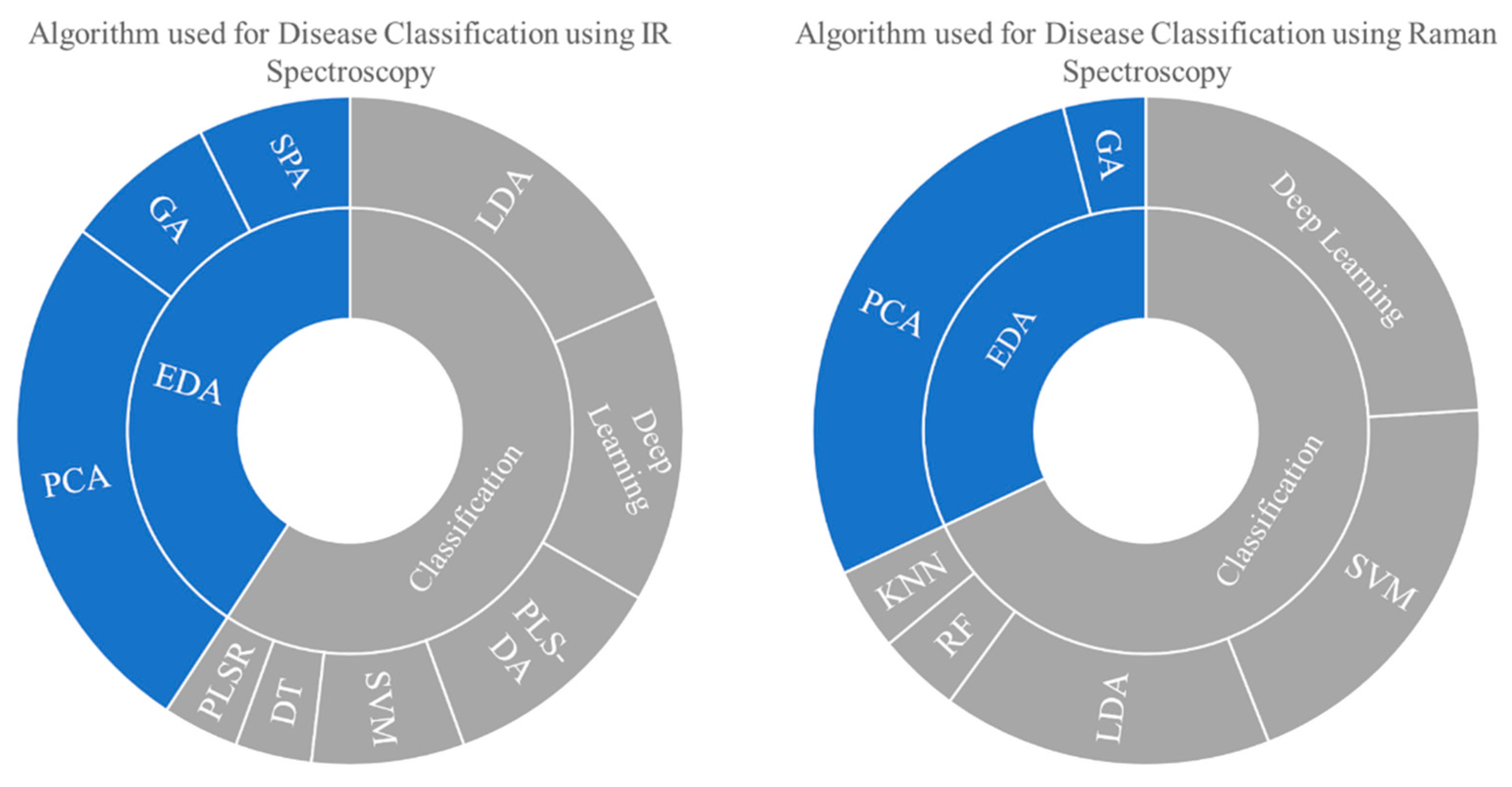
There are other spectroscopic methods; however, only the pattern recognition algorithms utilized in ultraviolet/visible (UV/Vis), infrared (IR), and Raman spectroscopy are covered here, including its general theories and past study within this domain. Due to the lack of relevant past studies on UV spectroscopy, Figure 2 only shows the algorithm mentioned for disease classification using IR and Raman spectroscopy.
5.1. Ultraviolet-Visible (UV/Vis) Spectroscopy
UV/Vis spectroscopy is used to determine the absorbance spectrum either in solution or as a solid. In actuality, it detects the absorption of light energy or electromagnetic radiation that excites electrons from their ground state to their initial singlet excited state.
5.1.1. General Theory of UV/Vis Spectroscopy
The ultraviolet/visible region of the electromagnetic spectrum spans 1.5–6.2 eV, corresponding to a wavelength range of 800–200 nm. UV/Vis spectroscopy data may provide qualitative and quantitative information about a particular substance or molecule. Regardless of whether quantitative or qualitative information is desired, it is critical to zero the instrument for the solvent in which the molecule is dissolved. UV/Vis spectroscopy works well on liquids and solutions, however, if the sample is a suspension of solid particles in a liquid, the sample will scatter more light than it absorbs, resulting in highly skewed results. UV/Vis equipment is often the most efficient in analyzing liquids and solutions.
5.1.2. Past Studies on UV/Vis Spectroscopy for Disease Classification
In contrast to other spectroscopy approaches, there has been a dearth of studies on sickness classification using UV/Vis spectroscopy. However, in the presence of agglutinating antibodies, this spectroscopic approach is often used to characterize blood, with predictable changes in the UV and visible light spectra of blood identifying the blood groups and types.
5.2. Infrared (IR) Spectroscopy
The infrared region of the mid- (fundamental) infrared (IR or MIR) has a wavenumber ranging from 4000 cm−1 (2.5 m) to 400 cm−1 (25 m). It is bounded by the far-IR region (FIR) spanning the wavelength range 400 cm−1 (25 m) to 10 cm−1 (1 mm) and the critical near-IR region (NIR) spanning the wavelength range 12,500 cm−1 (800 nm) to 4000 cm−1 (2.5 m). The most often used technique of spectroscopy is infrared spectroscopy. Numerous factors contribute to its enormous popularity and spread. The approach is speedy, sensitive, and simple to use, and it enables the sampling of gases, liquids, and solids using a variety of various procedures. Notable characteristics include the ease with which the spectra may be evaluated qualitatively and quantitatively [43].
5.2.1. General Theory of FTIR Spectroscopy
Infrared spectrometers or spectrophotometers of the modern era operated on a different principle. The architecture of the optical pathway creates a pattern. This is an interferogram because it is a complex signal with a wave-like pattern that spans the infrared spectrum. Individual absorption frequencies may be extracted from the interferogram using a mathematical procedure called the Fourier transform (FT), producing a virtually similar spectrum to that obtained by a dispersive spectrometer. A Fourier transform infrared (FTIR) spectrometer is a device that performs this function. The benefit of an FTIR instrument is that it takes less than a second to obtain the interferogram. Thus, hundreds of interferograms of the same sample may be collected and stored in a computer’s memory. A spectrum with a higher signal-to-noise ratio may be displayed when a Fourier transform is performed on the total of the collected interferograms. As a result, an FTIR instrument is more sensitive and faster than a dispersion instrument.
5.2.2. Past Study on IR Spectroscopy for Disease Classification
Table 2 shows an overview of selected past studies on pattern recognition for disease categorization through IR spectroscopy.
As shown in Table 2, almost all of the studies selected conduct exploratory data analysis prior to classification, with the exception of Yue et al. (2020), who used three deep learning models—a multilayer perceptron (MLP), a long-short-term memory network (LSTM), and a convolutional neural network (CNN)—to enable rapid diagnosis of abnormal thyroid function. As compared to typical machine learning algorithms, deep learning algorithms do not need data to be extracted artificially for features and perform better while processing big sample sets. The accuracy of the three models with the original data was 91.3 percent, 88.6 percent, and 89.3 percent, while the accuracy of the three models with the enhanced data was 92.7 percent, 93.6 percent, and 95.1 percent.
Ref. [16] researched the dengue virus’s concentration in blood and serum samples. Three distinct dimensional reduction techniques were applied (PCA, SPA, and GA) in conjunction with LDA. The research shows that, of the two samples, the blood sample provides the most accurate result, with 100% specificity and sensitivity. This finding prompted [45] to extend the work to the discrimination of various viruses in blood samples using similar algorithms. The findings indicated that the sensitivity and specificity of the healthy, dengue, and chikungunya classes were 100 percent, whereas zika had values close to 90 percent.
Ref. [47] conducted research on the diagnosis of Hepatitis B and Hepatitis C viruses by using three sample preparation procedures. Although ATR-FTIR appears to be a promising initial screening approach for detecting underlying infection and appears to be capable of discriminating HBV and HCV infected samples, the authors noted that the approach appears to detect the virus’s response to infection or the compounds synthesized by the virus, rather than the virus itself. As a result, further research is needed to determine the specificity of the response to various viruses and other infectious agents.
Ref. [48] use FTIR spectroscopy in conjunction with a machine learning approach to evaluate the characteristic spectra of salivary exosomes from oral cancer (OC) patients and healthy individuals (HI). This establishes a new platform for utilizing FTIR spectroscopy for the early detection of oral cancer. With a sensitivity of 100%, specificity of 89%, and accuracy of 95%, the PCA–LDA discrimination model accurately identified the samples, while the SVM had a training accuracy of 100% and cross-validation accuracy of 89%.
Ref. [54] also conducted research on the use of FTIR for dengue diagnosis; this is the first report of the use of freeze-dried human blood sera for FTIR analysis, according to the authors. They employed PCA to extract features and LDA to classify, resulting in a sensitivity and specificity of 89 and 95 percent, respectively. Following that, with an R2 = 0.9980 accuracy, the PLSR model was effectively employed to predict infection indications based on biochemical changes in blood samples. Then, in [52], another research was undertaken to discriminate typhoid and dengue illness using the same methodologies but without the PLSR, obtaining 100 percent accuracy between samples. Ref. [50] employed PCA as a dimensionality reduction technique in conjunction with three models to develop a method for rapidly detecting gliomas in human blood. In this research, a non-linear SVM with a radial basis function (RBF) kernel was used in conjunction with a Back Propagation Neural Network (BPNN) and DT. As a consequence, DT accuracy was determined to be quite poor, but PSO-SVM performed the best, with an accuracy of 92.00 percent and an AUC value of 0.919.
Ref. [51] uses two models based on PLS-DA to identify Aspergillus species in blood plasma in the presence of potential confounders found in patients at risk of invasive blood Aspergillosis, most notably the presence of commonly used drugs and common bloodstream pathogens in these patients. The basic model performs well in terms of prediction accuracy, with a total accuracy of 84.4 percent, while oversampling and autoscaling increase this to 93.3 percent.
Ref. [53] study the possibility of diagnosing Alzheimer’s disease (AD) utilizing spectral feature fusion technology and the PLS-DA classification approach. The accuracy, sensitivity, and specificity of the NIR-based PLS-DA model are 80.6 percent, 93.3 percent, and 93.7 percent, respectively, while the MIR-based PLS-DA model has values of 98.5 percent, 97.5 percent, and 100 percent. The equivalents for the PLS-DA model based on NIR-MIR spectral feature fusion are 100%, 97.5 percent, and 100%, respectively.
5.3. Raman Spectroscopy
Raman spectroscopy is a vibrational spectroscopic technique that is complementary to IR spectroscopy. Both have a similar wavelength range, but unlike IR spectroscopy which absorbs light by vibrating molecules, Raman on the other hand scatters light by vibrating molecules [5].
5.3.1. General Theory of Raman Spectroscopy
Raman spectroscopy, like other spectroscopy methods, identifies specific light-matter interactions. This approach, in particular, makes use of the fact that Stokes and anti-Stokes scattering exist to investigate molecule structure. Raman spectroscopy quantifies the energy difference between incoming and scattered photons caused by Stokes and anti-Stokes transitions. This is commonly expressed as a shift in the incident light source’s wavenumber. Because Raman detects changes in wavenumber, it may be utilized with any wavelength of light; however, near infrared and visible light are often employed. Ultraviolet photons may also be used; however, they often result in photodecomposition of the material. Infrared spectroscopy determines the wavenumber at which a functional group exhibits a vibrational mode, while Raman spectroscopy measures the vibrational shift caused by an incident source.
5.3.2. Past Studies on Raman Spectroscopy for Disease Classification
Table 3 shows the past studies on pattern recognition for disease classification using Raman spectroscopy.
As is the case with other spectroscopic approaches, PCA continues to dominate the EDA algorithm. Classification of Raman spectra data has been accomplished using a variety of techniques. SVM and LDA lead the other algorithms in the publications listed in Table 3.
Ref. [54] used Raman spectroscopy and SVM to analyze dengue infection in human blood sera. The SVM model was constructed using three distinct kernel functions: the RBF, polynomial, and linear. The polynomial kernel of order 1 exhibits the highest performance, with a diagnostic accuracy of around 85%, precision of 90%, sensitivity of 73%, and specificity of 93%. Then, Ref. [57] did a research study to distinguish between two distinct human pathogenic illnesses, typhoid, and dengue, that share certain clinical symptoms. Although the precise numbers are not provided in the research, the PCA-LDA model seems to provide adequate diagnostic accuracy and sensitivity.
Ref. [55] offers an investigation of hepatitis B virus (HBV) infection in human blood serum using Raman spectroscopy in conjunction with an SVM model with two alternative kernels (polynomial function and RBF) and two different optimization techniques (Quadratic programming and least square). The best classification performance is obtained with a second-order polynomial kernel which has a diagnostic accuracy of around 98 percent, precision of 97 percent, sensitivity of 100 percent, and specificity of 95 percent. Then, using Raman spectroscopy, Ref. [56] also explains how to analyze biochemical changes in human blood serum infected with HBV. The diagnostic accuracy of 99.3 percent, the sensitivity of 99.2 percent, the specificity of 99.4 percent, the positive predictive value of 99.2 percent, and the negative predictive value of 99.4 percent are achieved when a neural network classifier is used. Ref. [59] reported a technique for diagnosing HBV that incorporates serum Raman spectroscopy and a multiscale convolution independent circulation neural network (MSCIR). PCA was used to reduce the dimensions, and then the LDA, KNN, SVM, RF, ANN, and MSCIR algorithms were used, with their respective accuracies of 80.77%, 77.69%, 89.23%, 86.92%, 91.53%, and 96.15% demonstrating that the MSCIR is superior to the other.
Ref. [18] employed the PCA, LDA, and PLSR to predict viral load in human plasma samples for hepatitis C infection. Diagnostic sensitivity and specificity for the combined set of normal and variable viral load samples were 98.8 percent and 98.6 percent, respectively, for the combined set of normal and variable viral load samples, with a corresponding Positive Predictive Value of 99.2 percent and Negative Predictive Value of 98 percent.
With 99.8 percent accuracy, the PLSR model predicts the viral loads of HCV-infected plasma based on biochemical changes produced by viral infection. Another research was done on the detection of Hepatitis C in human blood serum, using SVM as the classification model. Despite the lack of an EDA method, the model achieves a total accuracy rate of 91.1 percent.
Ref. [60] performed a research study using Raman spectroscopy and a convolutional neural network to detect chronic renal failure.
The spectra were classified using a CNN and an Improved AlexNet, with an accuracy of 79.44% and 95.22%, respectively. Furthermore, the inclusion of noise had no discernible effect on categorization accuracy. This resulted in a conclusion that the accuracy of CNN in this research may be as high as 95.22 percent, a significant improvement above the previous study’s accuracy and dependability of 89.7 percent. A research study was also undertaken to distinguish echinococcosis and liver cirrhosis in healthy volunteers [21]. PCA and LDA were applied, and the algorithm’s total diagnosis accuracy was 87.7 percent. The diagnostic sensitivities to healthy volunteers, echinococcosis patients, and liver cirrhosis patients were 92.5 percent, 81.5 percent, and 89.1 percent, respectively, while the specificities were 93.2 percent, 96.1 percent, and 92.4 percent.
The majority of studies for illness categorization using spectroscopy employ blood or its components as the medium. However, different biofluids have also been employed. Ref. [62] conducted research to diagnose Alzheimer’s disease by analyzing cerebrospinal fluid. PCA and GA are employed as EDA algorithms, while ANN and SVM-DA are used for classification, yielding a sensitivity and specificity of 84%.
6. Initial Experimental Analysis of the Classification of Spectra Data
In order to obtain the best model, the classification analysis requires more than one step. The common pipeline used in classifying spectra data are data acquisition, data preprocessing, dimensionality reduction, modeling, and evaluation. As an example of the analysis of the classification algorithm in classifying spectral data, Attenuated Total Reflectance (ATR) FTIR dataset for ovarian cancer in urine was used. The dataset used was from a study by [63], which can be obtained from the publicly accessible data repository Figshare (https://figshare.com/articles/Potential_of_mid-infrared_spectroscopy_as_a_non-invasive_diagnostic_test_for_endometrial_or_ovarian_cancer_in_urine/5929516, accessed on 7 April 2022). The full data set consists of of 100 samples each from healthy individuals, patients with ovarian cancer and patient with endometrial cancer. In this paper, however, the preprocessed sample from healthy individuals and patients with ovarian cancer are used.
Throughout the experiments, the dataset was divided into training (n = 120 samples, 60 percent) and testing (n = 80 samples, 40 percent) sets. The practitioner determined the ratio of training to testing. In addition to the train-test split technique, any relevant cross-validation methodology may be used as an alternative to dividing the data. Then standard scaler was used on both sets in order to resize the distribution of data such that the mean of the observed values was 0 and the standard deviation was 1 respectively. LDA, SVM, and RF were selected among all classification models discussed in this study. PCA was also used to reduce dimensionality. This was due to the fact that LDA also functions as a dimensionality reduction method, PCA will only be done before SVM and RF. The RBF kernel will be implemented for SVM in the experiment conducted, and 100 estimators will be used in RF. After model training was complete, the testing set was used to compare the performance metrics of each model. Accuracy, sensitivity, and specificity were utilized as performance indicators. The results are shown in Table 4.
The classification performance achieved for the LDA, PCA-SVM, and PCA-RF models is shown in Table 4, and its graphical representation is depicted in Figure 3. LDA achieved 98.75 percent accuracy, 100 percent sensitivity, and 97.50 percent specificity. The accuracy, sensitivity, and specificity of PCA-SVM were all 97.50 percent. Finally, PCA-RF received a 95 percent accuracy rating, a 97.50 percent sensitivity rating, and a 92.50 percent specificity rating. Based on the results, LDA was superior to the other two classification models, PCA-SVM and PCA-RF, the latter being the weakest of the three.
7. Conclusions
In recent years, the application of pattern recognition in classifying human diseases using spectral analysis has increased. This study described a few of the most well-known and widely used methods for exploratory data analysis and classification. The advantages and disadvantages of the selected method were also briefly examined. Despite the fact that new algorithms have been developed throughout time, the majority of academics continue to employ the same set of algorithms that existed more than a decade ago. This is sensible, considering that the vast majority of researchers, especially those who are not experts in computer-related fields, would select a widespread and well-known technique.
A further justification for using the classical technique is that it performs better with smaller data sets. Currently, the most modern techniques are more data efficient. However, not all data are publicly accessible and may be accessed in vast quantities. Classical procedures are preferred over more complex techniques in this circumstance. In conclusion, classical methods are both computationally and financially inexpensive. The more complex a method is, the more resources will be necessary to implement it, both in terms of the amounts indicated before and the hardware used. This consists of a respectable high-end GPU, speedier RAMs, and a huge SSD storage capacity that meets the algorithm’s needs.
Consider the use of basic or traditional machine learning. In this scenario, it is recommended that the dimensionality of the data be decreased prior to enhancing the model’s overall performance using a classification technique. Dimensionality reduction may not be necessary for classification techniques such as ANN and deep learning. Regarding the categorization aspect of the study, each model has its own set of assumptions; hence, not every model will be appropriate for use with every dataset. Despite the fact that spectrum data have their characteristics, whether or not the model complements the dataset ultimately depends on the data.
Based on this review, a study to identify the presence of Coronavirus (COVID-19) positive utilizing spectrum analysis employing three spectroscopy techniques: IR Spectroscopy, UV Spectroscopy, and Raman Spectroscopy, in combination with pattern recognition algorithms, could be explored in the future. Each methodology revealed an excellent potential for creating alternative methods for identifying the presence of disease by utilizing the region of each radiation employed and classifying them using the best suitable algorithm based on the data provided. Apart from the algorithms mentioned in this paper, there are many other types of algorithms available today, resulting in an infinite number of ways to supplement spectroscopic approaches. An idea for a new way to detect the presence of COVID-19 disease would be a huge step forward in this field of research.
Author Contributions
Conceptualization, N.H.H. and A.B.; investigation, N.H.H.; writing—original draft preparation, N.H.H.; writing—review and editing, A.B., F.P.C. and M.I.R.; visualization, N.H.H.; supervision, A.B. and F.P.C.; project administration, A.B. and F.P.C.; funding acquisition, A.B., F.P.C. and M.I.R. All authors have read and agreed to the published version of the manuscript.
Funding
The research was funded by Universiti Malaysia Sabah grant number SDK0163-2020 and the APC was funded by Universiti Malaysia Sabah.
Institutional Review Board Statement
Not applicable.
Informed Consent Statement
Not applicable.
Data Availability Statement
Not applicable.
Acknowledgments
The authors would like to express their appreciation to Universiti Malaysia Sabah for funding this research study and publication through a grant with the code SDK0163-2020.
Conflicts of Interest
The authors declare no conflict of interest.
References
- Bishop, C.M. Pattern Recognition and Machine Learning; Springer: Berlin/Heidelberg, Germany, 2006. [Google Scholar]
- Mitchell, T.M. Machine Learning; McGraw-Hill: New York, NY, USA, 1997. [Google Scholar]
- Otto, M. Chemometrics: Statistics and Computer Application in Analytical Chemistry, 3rd ed.; Wiley-VCH Verlag GmbH & Co.: Weinheim, Germany, 2017. [Google Scholar]
- Ahmed, N.; Dawson, M.; Smith, C.; Wood, E. Biology of Disease, 1st ed.; Taylor & Francis Group: Abingdon-on-Thames, UK, 2007. [Google Scholar]
- Nielsen, S.S. Food Analysis, 5th ed.; Springer: Cham, Switzerland, 2017. [Google Scholar]
- Santos, M.C.D.; Nascimento, Y.M.; Araújo, J.M.G.; Lima, K.M.G. ATR-FTIR spectroscopy coupled with multivariate analysis techniques for the identification of DENV-3 in different concentrations in blood and serum: A new approach. RSC Adv. 2017, 7, 25640–25649. [Google Scholar] [CrossRef] [Green Version]
- Sammut, C.; Webb, G.I. Encyclopedia of Machine Learning; Springer: New York, NY, USA, 2010. [Google Scholar]
- Sumithra, V.S.; Surendran, S. A computational geometric approach for overlapping community (cover) detection in social network. In Proceedings of the 2015 International Conference on Computing and Network Communications (CoCoNet), Trivandrum, India, 16–19 December 2015; pp. 98–103. [Google Scholar]
- Anowar, F.; Sadaoui, S.; Selim, B. Conceptual and empirical comparison of dimensionality reduction algorithms (PCA, KPCA, LDA, MDS, SVD, LLE, ISOMAP, LE, ICA, t-SNE). Comput. Sci. Rev. 2021, 40, 100378. [Google Scholar] [CrossRef]
- Olver, P.; Shakiban, C. Applied Linear Algebra, 2nd ed.; Springer International Publishing AG: Cham, Switzerland, 2018. [Google Scholar]
- Raschka, S.; Mirjalili, V. Python Machine Learning, 3rd ed.; Packt Publishing Ltd.: Birmingham, UK, 2019. [Google Scholar]
- Kumar, R.; Sharma, V. Chemometrics in forensic science. Trends Anal. Chem. 2018, 105, 191–201. [Google Scholar] [CrossRef]
- Zimmer, V.A.M.; Fonolla, R.; Lekadir, K.; Piella, G.; Hoogendoorn, C.; Frangi, A.F. Patient-Specific Manifold Embedding of Multispectral Images Using Kernel Combinations. Mach. Learn. Med. Imaging 2013, 8184, 82–89. [Google Scholar] [CrossRef]
- Vidal, R.; Ma, Y.; Sastry, S.S. Generalized Principal Component Analysis; Springer: New York, NY, USA, 2016. [Google Scholar] [CrossRef]
- Araújo, M.C.U.; Saldanha, T.C.B.; Galvão, R.K.H.; Yoneyama, T.; Chame, H.C.; Visani, V. The successive projections algorithm for variable selection in spectroscopic multicomponent analysis. Chemom. Intell. Lab. Syst. 2001, 57, 65–73. [Google Scholar] [CrossRef]
- Santos, M.C.D.; Morais, C.L.M.; Nascimento, Y.M.; Araujo, J.M.G.; Lima, K.M.G. Spectroscopy with computational analysis in virological studies: A decade (2006–2016). Trends Anal. Chem. 2017, 97, 244–256. [Google Scholar] [CrossRef]
- Jarvis, R.M.; Goodacre, R. Genetic algorithm optimization for pre-processing and variable selection of spectroscopic data. Bioinformatics 2005, 21, 860–868. [Google Scholar] [CrossRef] [Green Version]
- Nawaz, H.; Rashid, N.; Saleem, M.; Asif Hanif, M.; Irfan Majeed, M.; Amin, I.; Iqbal, M.; Rahman, M.; Ibrahim, O.; Baig, S.M.; et al. Prediction of viral loads for diagnosis of Hepatitis C infection in human plasma samples using Raman spectroscopy coupled with partial least squares regression analysis. J. Raman Spectrosc. 2017, 48, 697–704. [Google Scholar] [CrossRef]
- Höskuldsson, A. PLS regression methods. J. Chemom. 1988, 2, 211–228. [Google Scholar] [CrossRef]
- Sharma, V.; Kumar, R. Trends of chemometrics in bloodstain investigations. Trends Anal. Chem. 2018, 107, 181–195. [Google Scholar] [CrossRef]
- James, G.; Witten, D.; Hastie, T.; Tibshirani, R. An Introduction to Statistical Learning; Springer: New York, NY, USA, 2013. [Google Scholar]
- Alfeilat, H.A.A.; Hassanat, A.B.A.; Lasassmeh, O.; Tarawneh, A.S.; Alhasanat, M.B.; Eyal Salman, H.S.; Prasath, V.B.S. Effects of Distance Measure Choice on K-Nearest Neighbor Classifier Performance: A Review. Big Data 2019, 7, 221–248. [Google Scholar] [CrossRef] [PubMed] [Green Version]
- Miller, J.N.; Miller, J.C. Statistics and Chemometrics for Analytical Chemistry, 6th ed.; Pearson Education Limited: Edinburgh Gate, UK, 2016. [Google Scholar]
- Boonamnuay, S.; Kerdprasop, N.; Kerdprasop, K. Classification and Regression Tree with Resampling for Classifying Imbalanced Data. Int. J. Mach. Learn. Comput. 2018, 8, 336–340. [Google Scholar] [CrossRef]
- Duda, R.O.; Hart, P.E.; Stork, D.G. Pattern Classification, 2nd ed.; Wiley: Somerset, NJ, USA, 2012. [Google Scholar]
- Maimon, O.; Rokach, L. Data Mining and Knowledge Discovery Handbook; Springer: New York, NY, USA, 2010. [Google Scholar]
- Quinlan, J.R. C4.5: Programs for Machine Learning; Morgan Kaufmann Publishers, Inc.: Los Altos, CA, USA, 1993. [Google Scholar]
- Zhang, C.; Ma, Y. Ensemble Machine Learning: Methods and Applications; Springer: New York, NY, USA, 2012. [Google Scholar]
- Boser, B.E.; Guyon, I.M.; Vapnik, V.N. A training algorithm for optimal margin classifiers. In Proceedings of the Fifth Annual Workshop on Computational Learning Theory, Pittsburgh, PA, USA, 27–29 July 1992; pp. 144–152. [Google Scholar] [CrossRef]
- Cortes, C.; Vapnik, V. Support-vector networks. Mach. Learn. 1995, 20, 273–297. [Google Scholar] [CrossRef]
- Lampropoulos, A.S.; Tsihrintzis, G.A. Machine Learning Paradigms; International Publishing: New York, NY, USA, 2015. [Google Scholar]
- Goodfellow, I.; Bengio, Y.; Courville, A. Deep Learning; The MIT Press: Cambridge, MA, USA, 2017. [Google Scholar]
- Clarke, B.; Fokoue, E.; Zhang, H.H. Principles and Theory for Data Mining and Machine Learning; Springer: New York, NY, USA, 2009. [Google Scholar]
- Zhang, Y.; Li, J.; Hong, M.; Man, Y. Applications of Artificial Intelligence in Process Systems Engineering; Elsevier: Amsterdam, The Netherlands, 2021. [Google Scholar]
- Fordellone, M.; Vichi, M. Finding groups in structural equation modeling through the partial least squares algorithm. Comput. Stat. Data Anal. 2020, 147, 106957. [Google Scholar] [CrossRef]
- Ruiz-Perez, D.; Guan, H.; Madhivanan, P.; Mathee, K.; Narasimhan, G. So you think you can PLS-DA? BMC Bioinform. 2020, 21, 2. [Google Scholar] [CrossRef]
- Popovic, A.; Morelato, M.; Roux, C.; Beavis, A. Review of the most common chemometric techniques in illicit drug profiling. Forensic Sci. Int. 2019, 302, 109911. [Google Scholar] [CrossRef]
- Basheer, I.A.; Hajmeer, M. Artificial neural networks: Fundamentals, computing, design, and application. Journal of Microbiological Methods 2001, 43, 3–31. [Google Scholar] [CrossRef]
- Tharwat, A. Classification assessment methods. Appl. Comput. Inform. 2020, 17, 168–192. [Google Scholar] [CrossRef]
- Japkowicz, N. Why question machine learning evaluation methods? In AAAI 2006 Workshop on Evaluation Methods for Machine Learning; AAAI: Menlo Park, CA, USA, 2006; pp. 6–11. [Google Scholar]
- Hand, D.J.; Till, R.J. A Simple Generalisation of the Area Under the ROC Curve for Multiple Class Classification Problems. Mach. Lang. 2001, 45, 171–186. [Google Scholar] [CrossRef]
- Jin Huang Ling, C.X. Using AUC and accuracy in evaluating learning algorithms. IEEE Trans. Knowl. Data Eng. 2005, 17, 299–310. [Google Scholar] [CrossRef] [Green Version]
- Gauglitz, G.; Vo-Dinh, T. Handbook of Spectroscopy; Wiley: Hoboken, NJ, USA, 2001. [Google Scholar]
- Banwell, C.N. Fundamentals of Molecular Spectroscopy; McGraw-Hill: London, UK, 1983. [Google Scholar]
- Santos, M.C.D.; Nascimento, Y.M.; Monteiro, J.D.; Alves, B.E.B.; Melo, M.F.; Paiva, A.A.P.; Pereira, H.W.B.; Medeiros, L.G.; Morais, I.C.; Fagundes Neto, J.C.; et al. ATR-FTIR spectroscopy with chemometric algorithms of multivariate classification in the discrimination between healthy vs. dengue vs. chikungunya vs. zika clinical samples. Anal. Methods 2018, 10, 1280–1285. [Google Scholar] [CrossRef]
- Naseer, K.; Ali, S.; Mubarik, S.; Hussain, I.; Mirza, B.; Qazi, J. FTIR spectroscopy of freeze-dried human sera as a novel approach for dengue diagnosis. Infrared Phys. Technol. 2019, 102, 102998. [Google Scholar] [CrossRef]
- Roy, S.; Perez-Guaita, D.; Bowden, S.; Heraud, P.; Wood, B.R. Spectroscopy goes viral: Diagnosis of hepatitis B and C virus infection from human sera using ATR-FTIR spectroscopy. Clin. Spectrosc. 2019, 1, 100001. [Google Scholar] [CrossRef]
- Zlotogorski-Hurvitz, A.; Dekel, B.Z.; Malonek, D.; Yahalom, R.; Vered, M. FTIR-based spectrum of salivary exosomes coupled with computational-aided discriminating analysis in the diagnosis of oral cancer. J. Cancer Res. Clin. Oncol. 2019, 145, 685–694. [Google Scholar] [CrossRef]
- Yue, F.; Chen, C.; Yan, Z.; Chen, C.; Guo, Z.; Zhang, Z.; Chen, Z.; Zhang, F.; Lv, X. Fourier transform infrared spectroscopy combined with deep learning and data enhancement for quick diagnosis of abnormal thyroid function. Photodiagnosis Photodyn. Ther. 2020, 32, 101923. [Google Scholar] [CrossRef]
- Chen, F.; Meng, C.; Qu, H.; Cheng, C.; Chen, C.; Yang, B.; Gao, R.; Lv, X. Human serum mid-infrared spectroscopy combined with machine learning algorithms for rapid detection of gliomas. Photodiagnosis Photodyn. Ther. 2021, 35, 102308. [Google Scholar] [CrossRef]
- Elkadi, O.A.; Hassan, R.; Elanany, M.; Byrne, H.J.; Ramadan, M.A. Identification of Aspergillus species in human blood plasma by infrared spectroscopy and machine learning. Spectrochim. Acta Part A Mol. Biomol. Spectrosc. 2021, 248, 119259. [Google Scholar] [CrossRef]
- Naseer, K.; Ali, S.; Qazi, J. ATR-FTIR spectroscopy based differentiation of typhoid and dengue fever in infected human sera. Infrared Phys. Technol. 2021, 114, 103664. [Google Scholar] [CrossRef]
- Yang, C.; Guang, P.; Li, L.; Song, H.; Huang, F.; Li, Y.; Wang, L.; Hu, J. Early rapid diagnosis of Alzheimer’s disease based on fusion of near- and mid-infrared spectral features combined with PLS-DA. Optik 2021, 241, 166485. [Google Scholar] [CrossRef]
- Naseer, K.; Amin, A.; Saleem, M.; Qazi, J. Raman spectroscopy based differentiation of typhoid and dengue fever in infected human sera. Spectrochim. Acta Part A Mol. Biomol. Spectrosc. 2019, 206, 197–201. [Google Scholar] [CrossRef]
- Khan, S.; Ullah, R.; Khan, A.; Wahab, N.; Bilal, M.; Ahmed, M. Analysis of dengue infection based on Raman spectroscopy and support vector machine (SVM). Biomed. Opt. Express 2016, 7, 2249. [Google Scholar] [CrossRef] [PubMed]
- Khan, S.; Ullah, R.; Khan, A.; Ashraf, R.; Ali, H.; Bilal, M.; Saleem, M. Analysis of hepatitis B virus infection in blood sera using Raman spectroscopy and machine learning. Photodiagnosis Photodyn. Ther. 2018, 23, 89–93. [Google Scholar] [CrossRef] [PubMed]
- Khan, S.; Ullah, R.; Ashraf, R.; Khan, A.; Khan, S.; Ahmad, I. Optical screening of hepatitis-B infected blood sera using optical technique and neural network classifier. Photodiagnosis Photodyn. Ther. 2019, 27, 375–379. [Google Scholar] [CrossRef] [PubMed]
- Cheng, H.; Xu, C.; Zhang, D.; Zhang, Z.; Liu, J.; Lv, X. Multiclass identification of hepatitis C based on serum Raman spectroscopy. Photodiagnosis Photodyn. Ther. 2020, 30, 101735. [Google Scholar] [CrossRef] [PubMed]
- Lu, H.; Tian, S.; Yu, L.; Lv, X.; Chen, S. Diagnosis of hepatitis B based on Raman spectroscopy combined with a multiscale convolutional neural network. Vib. Spectrosc. 2020, 37, 103038. [Google Scholar] [CrossRef]
- Gao, R.; Yang, B.; Chen, C.; Chen, F.; Chen, C.; Zhao, D.; Lv, X. Recognition of chronic renal failure based on Raman spectroscopy and convolutional neural network. Photodiagnosis Photodyn. Ther. 2021, 34, 102313. [Google Scholar] [CrossRef]
- Lü, G.; Zheng, X.; Lü, X.; Chen, P.; Wu, G.; Wen, H. Label-free detection of echinococcosis and liver cirrhosis based on serum Raman spectroscopy combined with multivariate analysis. Photodiagnosis Photodyn. Ther. 2021, 33, 102164. [Google Scholar] [CrossRef]
- Ryzhikova, E.; Ralbovsky, N.M.; Sikirzhytski, V.; Kazakov, O.; Halamkova, L.; Quinn, J.; Zimmerman, E.A.; Lednev, I.K. Raman spectroscopy and machine learning for biomedical applications: Alzheimer’s disease diagnosis based on the analysis of cerebrospinal fluid. Spectrochim. Acta Part A Mol. Biomol. Spectrosc. 2021, 248, 119188. [Google Scholar] [CrossRef]
- Paraskevaidi, M.; Morais, C.L.M.; Lima, K.M.G.; Ashton, K.M.; Stringfellow, H.F.; Martin-Hirsch, P.L.; Martin, F.L. Potential of mid-infrared spectroscopy as a non-invasive diagnostic test in urine for endometrial or ovarian cancer. Analyst 2018, 143, 3156–3163. [Google Scholar] [CrossRef]
Figure 1.
Region of the electromagnetic spectrum along with the corresponding type of quantum changes [44].
Figure 1.
Region of the electromagnetic spectrum along with the corresponding type of quantum changes [44].

Figure 2.
Algorithm mentioned for disease classification for IR and Raman spectroscopy in this study.
Figure 2.
Algorithm mentioned for disease classification for IR and Raman spectroscopy in this study.

Figure 3.
Performance comparison of LDA, PCA-SVM, and PCA-RF in classifying ATR-FTIR data of ovarian cancer in urine.
Figure 3.
Performance comparison of LDA, PCA-SVM, and PCA-RF in classifying ATR-FTIR data of ovarian cancer in urine.


Table 1.
Example of kernels used in SVM and its formula.
| Kernel | Formula |
|---|---|
| Linear | |
| Radial Basis Function (RBF) | |
| Polynomial | |
| Sigmoid |
, r, and d are kernel parameters.
Table 2.
Overview of selected past studies on pattern recognition for disease classification using IR spectroscopy.
Table 2.
Overview of selected past studies on pattern recognition for disease classification using IR spectroscopy.
| Year | Disease (Sample) | Aim of Research | EDA Algorithm | Classification Algorithm | Findings | References |
|---|---|---|---|---|---|---|
| 2017 | Dengue (Human blood and human sera) | Identification of DENV-3 in different concentrations in blood and serum | PCA, SPA, GA | LDA | Blood samples yield the best results with sensitivity and specificity: 100% | [6] |
| 2018 | Dengue, Chikungunya and Zika (Human blood) | Discrimination between healthy vs. dengue vs. chikungunya vs. zika clinical samples | PCA, SPA, GA | LDA | PCA-LDA Sensitivity: 100%; Specificity: 92%SPA-LDASensitivity: 100%; Specificity: 92% GA-LDA Sensitivity: 92%; Specificity: 86% | [45] |
| 2019 | Dengue (Freeze-dried human blood serum) | Discrimination of dengue positive and healthy serum samples by biochemical differences detected | PCA | LDA PLSR | Sensitivity: 89%; Specificity: 95%; R2 = 0.9980 | [46] |
| 2019 | Hepatitis B and Hepatitis C (Human blood serum) | Classification of human serum samples based on the presence of Hepatitis B virus and Hepatitis C virus infection | PLS-DA | Method 1 HBV vs. control sensitivity: 69.4% specificity: 73.7% HCV vs. control Sensitivity: 51.3% Specificity: 90.9% Method 2 HBV vs. control Sensitivity: 84.4% Specificity: 93.1% HCV vs. control Sensitivity: 80.0% Specificity: 97.2%, HBV vs. HCV Sensitivity: 77.4% Specificity: 83.3% Method 3 HBV vs. control (high molecular concentrate) Sensitivity: 87.5% Specificity: 94.9% HCV vs. control (high molecular concentrate) Sensitivity: 81.6% Specificity: 89.6% | [47] | |
| 2019 | Oral cancer (Saliva in pellet form) | Discrimination of FTIR spectra of salivary exosomes from oral cancer patients and healthy individuals | PCA | LDASVM | LDAAccuracy: 95%; Sensitivity: 100%; Specificity: 89% SVM Training accuracy: 100% Cross-validation accuracy: 89% | [48] |
| 2020 | Abnormal thyroid disease specifically hypothyroidism and hyperthyroidism (Human blood) | Diagnosis of abnormal thyroid disease in human blood samples | None | MLP, LSTM, CNN | Accuracy (original data) MLP: 91.3%, LSTM: 88.6%; CNN: 89.3%, Accuracy (with data enhancement) MLP: 92.7%; LSTM: 93.6%; CNN: 95.1% | [49] |
| 2021 | Human glioma (Human blood serum) | Identification of patients with gliomas | PCA | PSO-SVM, BPNN, DT | AccuracyPSO-SVM: 92.00% BPNN: 91.83% DT: 87.20%, | [50] |
| 2021 | Aspergillus species (Human blood plasma in kBr pellet form) | Identification of Aspergillus species in human blood plasma | Two models based on PLS-DA | Total accuracy of 84.4%, while oversampling and autoscaling improved this accuracy to 93.3%. | [51] | |
| 2021 | Typhoid and Dengue (Human blood serum) | PCA | LDA | Accuracy: 100% | [52] | |
| 2021 | Alzheimer’s Disease (Human blood serum) | Diagnosis of an individual with Alzheimer’s disease | PCA | PLS-DA | NIR Accuracy: 80.6%; Sensitivity: 93.3%; Specificity: 93.7% MIR Accuracy: 98.5%; Sensitivity: 97.5%; Specificity: 100% | [53] |
Table 3.
Overview of selected past studies on pattern recognition for disease classification using Raman spectroscopy.
Table 3.
Overview of selected past studies on pattern recognition for disease classification using Raman spectroscopy.
| Year | Disease (Sample) | Aim of Research | EDA Algorithm | Classification Algorithm | Findings | References |
|---|---|---|---|---|---|---|
| 2016 | Dengue Virus (Human Blood Sera) | Classification of dengue infected and normal healthy sera. | PCA | SVM with three different kernel functions (RBF, polynomial function, and linear function) | Best: SVM (RBF kernel with the polynomial kernel of order 1) Accuracy: 85%; Sensitivity: 73%; Specificity: 93% | [55] |
| 2017 | Hepatitis C (Human Plasma) | Identify the biochemical changes associated with the presence of the Hepatitis C virus in infected human blood plasma samples and healthy samples. | PCA | LDA | PCA-LDA Sensitivity: 98.8%; Specificity: 98.6% | [18] |
| 2018 | Hepatitis B (Human Blood) | Classification of hepatitis B virus infection in human blood serum | PCA | SVM with two different kernels, each with two different implementation methods has been used. | Best: SVM (RBF kernel with the polynomial kernel of order 2) Accuracy: 98%; Sensitivity: 100%; Specificity: 95% | [56] |
| 2019 | Hepatitis B (Human Blood Serum) | Classification of normal sera and pathological (hepatitis B infected) sera | None | NNC | Accuracy: 99.3; Sensitivity: 99.2; Specificity: 99.4 | [57] |
| 2019 | Dengue and Typhoid (Human Blood Serum) | Differentiation between typhoid and dengue in which both have some symptom similarity | PCA | LDA | The PCA-LDA model yielded sufficient diagnostic accuracy and sensitivity | [54] |
| 2020 | Hepatitis C (Human Blood Serum) | Classification of three kinds of serum Raman spectra (healthy people, hcv1 patients, and hcv2 patients) | None | SVM | Total Accuracy Rate: 91.1% | [58] |
| 2020 | Hepatitis B (Human Blood Serum) | Identification of patient infected with hepatitis B virus in human blood serum | PCA | LDA, KNN, SVM, RF, ANN, MSCIR | Model (Accuracy) LDA: 80.77%; KNN: 77.69%; SVM: 89.23%; RF: 86.92%; ANN: 91.53%; MSCIR: 96.15% | [59] |
| 2021 | Chronic Renal Failure (CRF) (Human Blood Serum) | Classification of normal blood serum and CRF infected blood serum | None | CNNImproved AlexNet | Improved AlexNet (Accuracy: 79.44%) CNN (Accuracy: 95.22%) | [60] |
| 2021 | Echinococcosis and liver cirrhosis (Human Blood Serum) | Discrimination of echinococcosis and liver cirrhosis from healthy volunteers | PCA | LDA | Overall Accuracy: 87.7% Healthy volunteers Sensitivity: 92.5%; Specificity: 93.2%, Patients with Echinococcosis Sensitivity: 81.5%; Specificity: 96.1%, Liver Cirrhosis Sensitivity: 89.1%; Specificity: 92.4% | [61] |
| 2021 | Alzheimer’s Disease (Cerebrospinal Fluid (CSF)) | Differentiation of CSF samples obtained from Alzheimer’s Disease patients and healthy controls. | PCA GA | ANN SVM-DA | Sensitivity & Specificity: 84% | [62] |
Table 4.
Classification performance obtained for LDA, PCA-SVM, and PCA-RF models.
| Classification Model | Accuracy (%) | Sensitivity (%) | Specificity (%) |
|---|---|---|---|
| LDA | 98.75 | 100.00 | 97.50 |
| PCA-SVM | 97.50 | 97.50 | 97.50 |
| PCA-RF | 95.00 | 97.50 | 92.50 |
Publisher’s Note: MDPI stays neutral with regard to jurisdictional claims in published maps and institutional affiliations. |
© 2022 by the authors. Licensee MDPI, Basel, Switzerland. This article is an open access article distributed under the terms and conditions of the Creative Commons Attribution (CC BY) license (https://creativecommons.org/licenses/by/4.0/).
Share and Cite
MDPI and ACS Style
Hasbi, N.H.; Bade, A.; Chee, F.P.; Rumaling, M.I. Pattern Recognition for Human Diseases Classification in Spectral Analysis. Computation 2022, 10, 96. https://0-doi-org.brum.beds.ac.uk/10.3390/computation10060096
AMA Style
Hasbi NH, Bade A, Chee FP, Rumaling MI. Pattern Recognition for Human Diseases Classification in Spectral Analysis. Computation. 2022; 10(6):96. https://0-doi-org.brum.beds.ac.uk/10.3390/computation10060096
Chicago/Turabian StyleHasbi, Nur Hasshima, Abdullah Bade, Fuei Pien Chee, and Muhammad Izzuddin Rumaling. 2022. "Pattern Recognition for Human Diseases Classification in Spectral Analysis" Computation 10, no. 6: 96. https://0-doi-org.brum.beds.ac.uk/10.3390/computation10060096
Note that from the first issue of 2016, this journal uses article numbers instead of page numbers. See further details here.