1. Introduction
Many porous media problems occur over multiple scales. Because of scale disparity, some type of model reduction or averaging are often employed. Typical flow-based upscaling approaches ([
1,
2,
3]) compute the permeabilities on a coarse (computational) grid and solve the flow and transport equations together on a coarse grid. These approaches are easy to implement with a minimal code modification; however, these approaches can result in large errors for complex heterogeneities because limited information is used in upscaling. In this paper, we consider a multiscale method for a coupled flow and transport system, where the flow equation for the pressure field is described by a steady state elliptic equation (derived by Darcy law) and the transport equation for the concentration field is described by a convection-dominated parabolic equation.
Our approach derives its foundation from rigorous multiscale techniques developed recently [
4,
5,
6,
7,
8,
9,
10,
11,
12,
13,
14,
15,
16,
17,
18,
19,
20,
21,
22,
23,
24,
25]. In our approach, multiscale basis functions are computed and used to solve flow equations. The main contributions of this paper are (1) to use multiscale basis functions for both flow and transport equations and (2) design of a novel mixed multiscale methods for convection-dominated transport equations within the context of Generalized Multiscale Finite Element Method (GMsFEM). The GMsFEM is introduced in [
16], where the objective is to construct multiscale basis functions in each coarse domain. The main distinction of this approach from some of existing multiscale methods is that the GMsFEM systematically constructs multiscale basis functions using local spectral problems and the local snapshot spaces. Both of these concepts (local spectral problem and local snapshot spaces) are important in a design of the method.
In our proposed approach, we use a mixed formulation for both the flow and the transport equations. The use of a mixed formulation for the flow equation guarantees the mass conservation [
7,
26,
27,
28,
29,
30]. The use of a mixed formulation is important for the transport equation, guarantees the mass conservation and helps with the stabilization of it. In particular, by adding more flux basis functions, we can achieve a better stability based on our numerical studies [
31]. In the mixed formulation for a coupled system, we first define snapshot spaces for the appropriately defined fluxes in the flow and the concentration equations. For the pressure and the concentration fields, we use piecewise constant basis functions. The snapshot space represents the solution space in each coarse region and provides a mass conservative approach. In the snapshot space, we perform a local spectral decomposition to identify multiscale basis functions. The functions corresponding to dominant modes are used to construct coarse spaces for the fluxes. In particular, we use only a few degrees of freedom (maximum two) in each coarse region. For the test functions for the convection-dominated transport, we use the solutions of adjoint problem. As a result, we have a full coarse-grid approximation for the coupled flow and transport system.
We would like to discuss a relation between our proposed approaches and the flow-based upscaling [
2,
3]. In the latter, the upscaled permeabilities are computed and, then, the coupled flow and transport equation is solved on a coarse grid. The computations of upscaled permeabilities can be compared to the computations of multiscale basis functions, which are performed locally in each coarse region by solving local problems. The resulting coarse-grid problem in the upscaled model is similar to our resulting coarse-grid system. There are several main advantages of the proposed method: (1) it can use more multiscale basis functions in each region and achieve a desired accuracy; (2) the number of multiscale basis functions can be adaptively selected in space and time; (3) our approach can easily reconstruct the fine-scale distributions of the solution; (4) our approaches can handle any coarse-grid geometries.
We consider several numerical examples by considering two different hydraulic conductivity fields. In our numerical examples, we use a relatively coarse grid with the coarsening factor of 20. We study the numerical errors in the concentration field and depict concentration profiles at different time instants. Our numerical results show that the use of only one basis function per coarse edge (which is similar to numerical upscaling of hydraulic conductivity) does not produce an accurate solution, while if we use two basis functions, we can obtain a much more accurate approximation of the solution. These preliminary numerical results show that our fully coarse-grid model for the coupled flow and transport equations can accurately predict the solution using only a few degrees of freedom in each coarse region.
Novelty. The novelty of our work can be summarized as follows:
The development of Generalized Multiscale Finite Element Method for a mixed formulation of the convection-diffusion equation using different test and trial spaces.
The development and implementation of a mass conservative mixed GMsFEM for the coupled flow and transport equations.
The paper is organized as follows. In the next section, we present preliminaries and describe coarse and fine grids as well as a mixed formulation.
Section 3 is devoted to the construction of multiscale basis functions. Numerical results are presented in
Section 4. Finally, we present conclusions.
2. Preliminaries and Notations
We consider a coupled flow and transport system that arises in many hydrological applications
Here Ω is the computational domain,
is a fixed time,
κ is a hydraulic conductivity,
c is the concentration,
p is the pressure,
D is a diffusivity of the medium, and
,
are source terms. The equations are subject to the boundary conditions
on
,
on
and the initial condition
in Ω. In order to have a mass conservation, we re-write the system in a mixed formulation.
Here q is an auxiliary variable, we call it flux or flux-concentration. It is well known that the Galerkin method inherits the stability of the continuous problem, and it yields to spurious oscillation when the convection coefficient is larger than the diffusive one (). The mixed finite element methods can be used to achieve a mass conservation. In this paper, we aim to construct multiscale basis functions for the flux q and the velocity v. As for the concentration c and the pressure p, we choose piecewise constant functions on a coarse grid.
Next, we introduce the discretized form of the Problem (
2). We first comment on some notations of the coarse and the fine mesh. We assume that Ω is partitioned in a usual way into a union of rectangles (in 2-D) or hexadedrals (in 3-D) denoted by
, where
H is the coarse mesh size. The fine mesh is obtained by splitting each coarse block in
into a connected union of fine-grid blocks, and we denote it by
with mesh size
h,
. In addition, we denote by
the set of all edges/faces of elements in
,
i.e.,
, where
is the number of coarse edges/faces. Note that each
is the union of some fine-grid edges/faces. That is,
, where
are the fine-grid edges/faces lying on
. We also define the coarse neighborhood of the edge/face
by
See
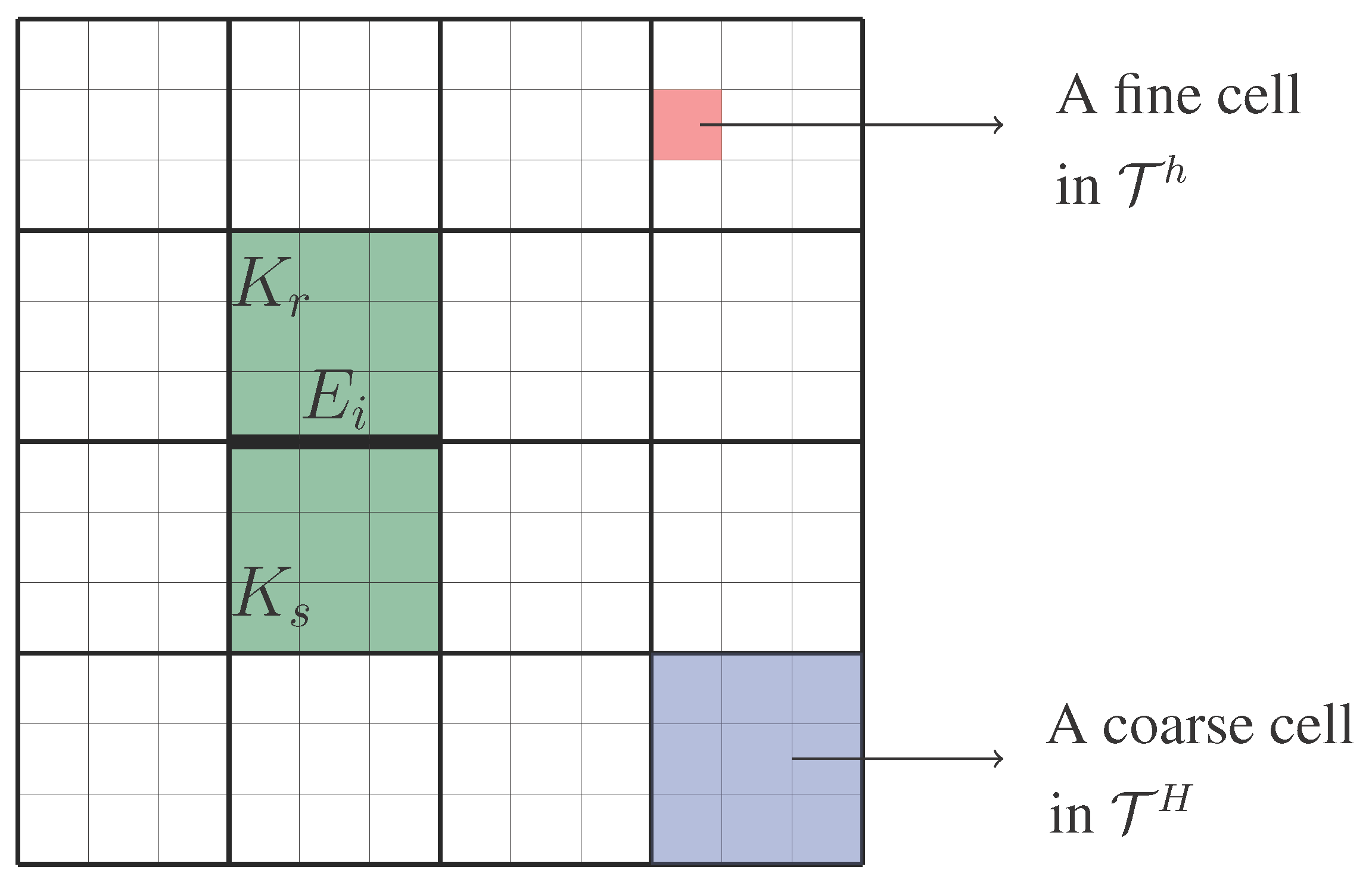
Figure 1 for an illustration of a coarse neighborhood associated with one coarse edge, where the coarse mesh and the fine mesh are represented by black lines and gray lines, respectively.
Figure 1.
An illustration of a coarse neighborhood (in green) corresponding to the coarse edge .
Figure 1.
An illustration of a coarse neighborhood (in green) corresponding to the coarse edge .
Next, we define the coarse trial spaces for
and
p. The concentration
c and the pressure
p are approximated in the space of piecewise constant functions with respect to the coarse grid
. We denote this space by
, and
As for the flux-concentration
q and the velocity
v, the basis functions are associated with coarse edges and are supported in the corresponding coarse neighborhoods. In particular, to obtain the basis functions for a coarse edge
, we will solve a local problem in the coarse neighborhood
. Let
and
be the set of multiscale basis functions for
q and
v with respect to
, respectively. Then, we define the multiscale solution space for
q and
v as
Furthermore, we discretize the time interval
uniformly by the points
where
τ is the time step and
. Using the above spaces, the GMsFEM approximation of (
2) can be given as follows. For all
, find
, such that
subject to the boundary condition
. Here, we let
, where
or
. For
and 1, we get the Backward Euler, Crank-Nicolson and Forward Euler Methods respectively. Note that
is the testing space for
. We emphasize that in general,
, which allows a better stability. The construction of
and
will be discussed in the next section.
In addition, to get the fine-scale solution, we use the standard lowest-order Raviart-Thomas space
for the approximation of (
2) on the fine grid
. The fine-scale solution
will be considered as a reference solution for the comparison with the multiscale solution
.
3. Generalized Multiscale Finite Element Method
In this section, we will discuss the construction of the vector solution spaces
, and the testing space
. Note that solving
in (
6) requires
. Therefore, we will first compute
using the last two equations of (
6).
We briefly introduce the basic idea of the GMsFEM. In the framework of GMsFEM, it follows an offline-online procedure to generate the multiscale solution space. At the offline stage, we first construct the snapshot space obtained by solutions of local problems with all possible boundary conditions, which are resolvable by the fine-grid. Then, we choose a subspace of the snapshot space by selecting dominant modes via some local spectral decompositions. The resulting reduced dimensional space, called the offline space, will be used at the online stage to get a multiscale solution. Note that the snapshot space can be taken as the solution space to obtain a solution with a good accuracy. However, it is expensive to use the snapshot space due to its high dimensionality. Thus, there is a need to perform a space reduction within the snapshot space, and choose only few dominant modes to form the offline space. We remark that for parameter dependent problems (in which the coefficients depend on some extra parameters), one needs to construct an online space using the offline space and an appropriate spectral problem.
3.1. Multiscale Solution Space
We form the multiscale solution space
for
. In order to build
, we first construct the snapshot space, denoted by
. For each coarse-grid edge
, a local problem is defined on each of its neighboring coarse cells. Because the snapshot space is supposed to capture the multiscale information within this local domain, the corresponding boundary conditions of the local problem should cover all possibilities. Formally, the local problem is defined as the following: For each
, on its neighboring coarse cell
or
(see
Figure 2), find
, such that
Here,
j varies over all fine-grid edges on
. For the convenience, we use the same notations as the solution to denote local snapshot fields. Here
is a constant defined on
K,
n is a fixed unit-normal vector on
, and
is defined on
with respect to the fine-grid edges. Note that
. We require
has value 1 on
and 0 on the other fine-grid edges,
, where
is the number of the fine-grid edges on
. That is,
Figure 2.
Neighboring coarse cells and corresponding to the coarse-grid edge . The fine-grid edge and are in red.
Figure 2.
Neighboring coarse cells and corresponding to the coarse-grid edge . The fine-grid edge and are in red.
Note that the constant
in (
7) is chosen so that the compatibility condition
is satisfied, for
or
. The above local Problem (
7) can be solved numerically on the underlying fine grid of
K by the lowest-order Raviart-Thomas element method.
After solving the local problems (on
and
) with respect to
, a local snapshot
is generated by the solutions of (
7). That is
Then, the snapshot space
is formed as
We re-numerate the snapshot functions by a single index to create the snapshot matrix
where
is the dimension of the snapshot space
. Note that the matrix
maps from the coarse space
to the fine space. The next step is to construct the offline space
for
. For a coarse-grid edge
, we define the following eigenvalue problem in
:
where
and
The eigenvalue Problem (
9) will produce a set of eigenvectors for generating the local offline space
by first selecting
eigenvectors corresponding to the smallest
eigenvalues, and then computing the element
for
, where
is the
j-th component of
. Then, the local offline space with respect to
is formed as
and the offline space
is formed as
We re-numerate the basis functions by a single index to create the offline matrix
where
is the dimension of the offline space
.
We take the multiscale solution space as
Then,
is approximated by solving the problem: Find
such that
subject to the boundary condition
.
Remark 1. The design of a ”good” eigenvalue problem is a key ingredient of the GMsFEM. It plays a critical role in reducing the dimension of the coarse solution space. After applying such eigenvalue problem, a few dominant modes are selected to capture the multiscale behavior of the multiscale solution up to some certain extent.
Remark 2. Generally, the offline space should contain a constant basis function. Therefore, the local snapshot space , as a solution space of the eigenvalue Problem (9), can be decomposed into , where and . We note that the element with in the snapshot space corresponds to the local solution with the unit normal flux on the edge and the elements of have average zero normal flux traces. We eliminate the constant boundary condition basis function in the snapshot space and put it, , as the first basis function of the offline space, and identify the other dominant modes in the space . 3.2. Multiscale Solution Space
We construct the solution space
and the testing space
for
. They follow a similar procedure to the one for
. In order to build
, the snapshot space
is to be constructed. We define a local problem corresponding to each coarse-grid edge
as follows: Find
, such that
where
or
depicted in
Figure 2. The local snapshot space
, the snapshot space
, and the snapshot matrix
are formed as
respectively.
To construct the testing space
, a snapshot space
is also needed. We solve the adjoint problem of (
12)
Then, the snapshot space is formed by the snapshot functions for all .
The local offline space
for
is obtained by solving the following eigenvalue problem in
:
where
and
Here, we let
where
denotes the vector
norm of
. Then, the local offline space
, the offline space
and the offline matrix
are formed as:
respectively. Here
,
, is the dominant mode in the space
We let
and define the testing space as
where
n is the unit-normal vector of the coarse-grid edge
E. Now, we have the multiscale solution space
and the testing space
. The GMsFEM solution
can be computed through (
6).
Remark 3. We remark that the fine-scale velocity field is constructed and used in computing multiscale basis functions for the concentration. In future, we plan to study joint multiscale basis construction procedures, which can compute multiscale basis functions for the concentration without solving the velocity field. Because the concentration field is a nonlinear function of the velocity field, an online procedure for computing multiscale basis functions for the concentration will be employed.
4. Numerical Results
We present a representative set of numerical experiments that demonstrate the performance of the mixed GMsFEM for approximating the coupled flow and transport Equation (
2). The computational domain Ω =
. We consider two different permeability fields
κ, as depicted in
Figure 3a,b. The source term
to be used are plotted in
Figure 3c,d, and
is chosen to be 0. In all experiments below, the fine grid
is fixed to be
uniform mesh,
i.e.,
. The coarse grid consists of
uniform meshes,
i.e.,
. As for the time discretization, the time step is chosen to be
and the Crank-Nicolson scheme is used. We denote
as the average value of
in each coarse cell,
i.e.,
, for every
. The relative numerical errors are measured in
norm for the concentration.
Figure 3.
Two permeability fields (a,b) and two source terms (c,d).
Figure 3.
Two permeability fields (a,b) and two source terms (c,d).
In our numerical experiments, we approximate the velocity and the flux (at any time instant) in the offline space and in which each coarse edge is equipped with basis functions. We choose at most and compare concentration profiles with . Note that there are basis functions associated with each coarse edge. We only select up to the two dominant modes per edge to form the offline space.
The first experiment is for the Problem (
2), where the diffusivity
, the source term
, the permeability field
, and the boundary condition
. The boundary condition represents the flow from lower left corner to upper right corner. The Peclet number in the entire domain is
, while the coarse-grid Peclet numbers vary with the maximum one being
. In
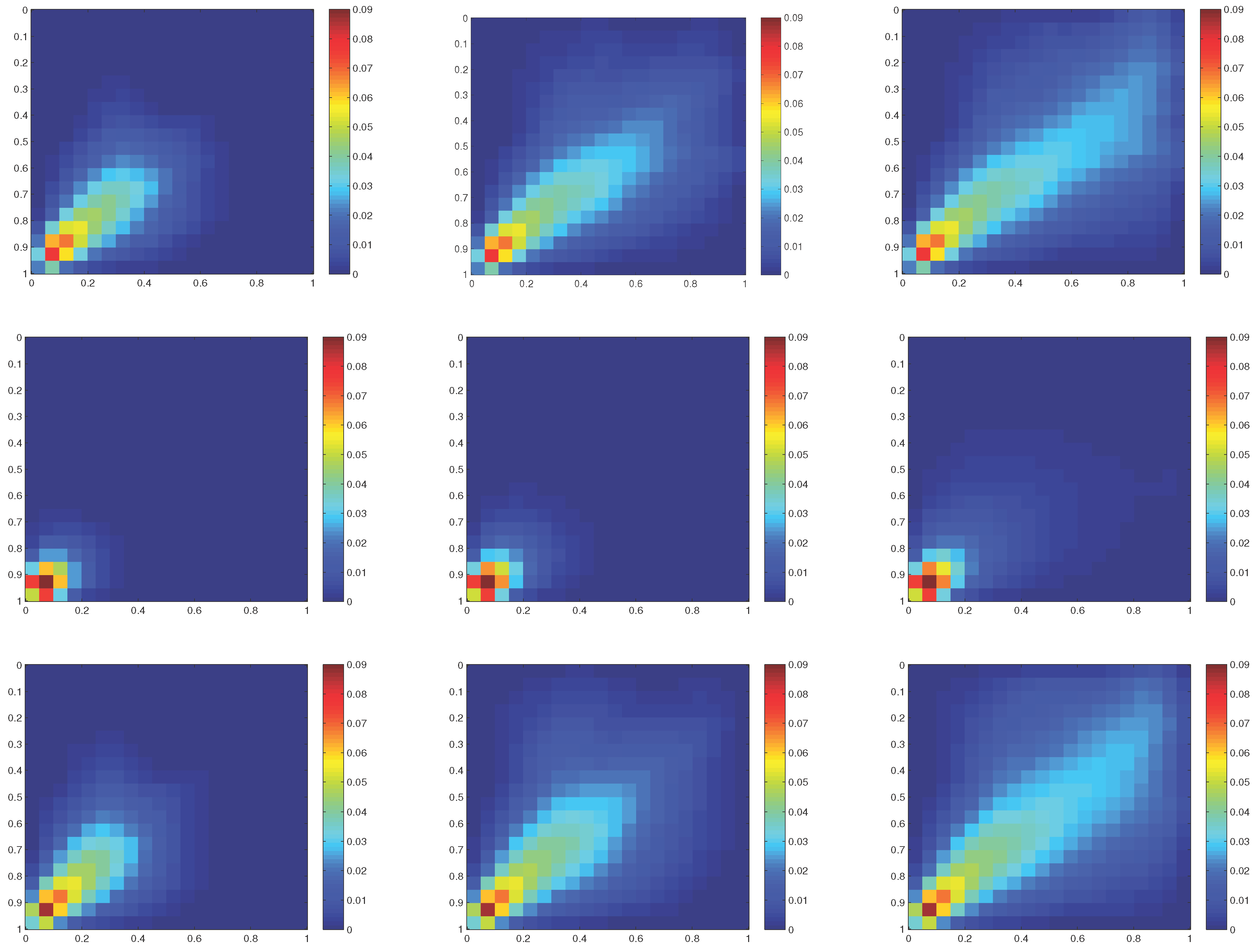
Figure 4, we depict the averaged fine-scale solutions and the GMsFEM solutions at the time
,
, and
. We choose the averaged fine-scale solution since piecewise constant basis functions are used in the approximation of the concentration on a coarse grid. The averaged fine-scale solution is depicted on the top of
Figure 4. In the middle row, we depict the GMsFEM solution, where only one basis function per edge is used for the approximation of the velocity and one basis function is used for the approximation of the flux-concentration field. The
errors in the concentration field are
%,
%, and
% at
,
, and
. At the bottom row of
Figure 4, we depict the concentrations computed using two basis functions for the velocity and two basis functions for the flux-concentration field. As we observe, the results look much better when two basis functions are used. For example, at
, we can observe that the concentration profile is similar to the averaged fine-scale concentration profile. The
errors in the concentration field are
%,
%, and
% at
,
, and
. Note that since we use
coarse grid and piecewise constant basis functions for the concentration, one expects a first order convergence with respect to the coarse mesh (
i.e., about 5% error in our case).
Figure 4.
First row: Fine-scale solutions . Second row: GMsFEM solutions (one multiscale basis function per edge for both velocity and flux-concentration). Third row: GMsFEM solutions (two multiscale basis function per edge for both velocity and flux-concentration). From left column to right column: . We use , , H = 1/20.
In our second set of numerical examples, we consider the permeability
, a source term
, and a boundary condition
. We let the diffusivity to be
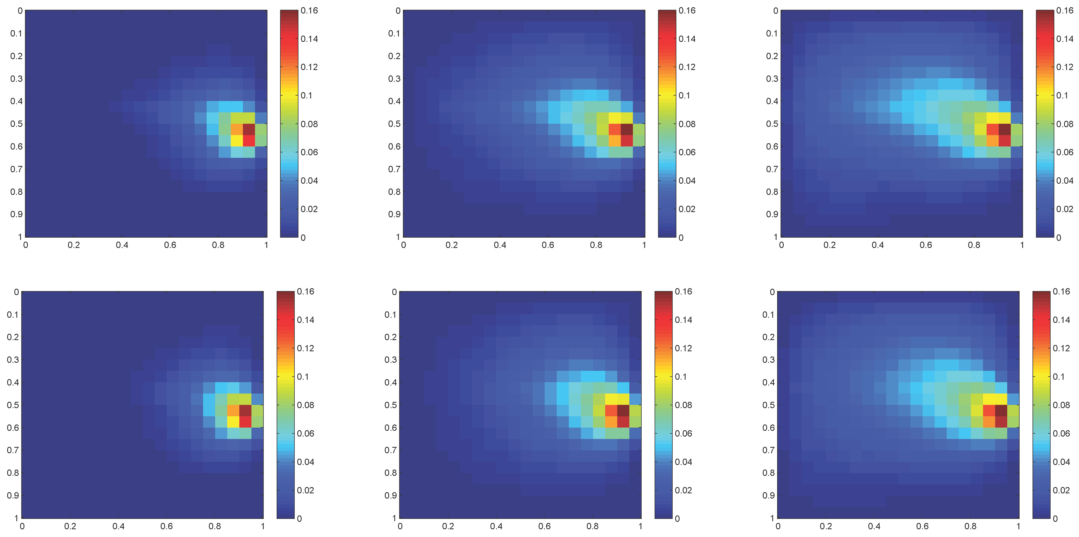
. In this case, the problem becomes convection-dominated, where the coarse-grid Peclet number has a maximum value around 8.1. The numerical results are shown in
Figure 5, where the top row shows the averaged fine-scale concentration profiles, the middle row shows the GMsFEM solution with one velocity basis per edge and one flux-concentration basis function, and the bottom row shows the GMsFEM solution, which uses two velocity basis functions and two flux-concentration basis functions. In all numerical results, we use piecewise constant pressure and piecewise constant concentration basis functions, as mentioned earlier. Thus, for the concentration field, there is an irreducible error of order
H (5% in our case). First, we study the numerical results using only one multiscale basis function (the middle row of
Figure 5). The
errors in the concentration field are
%,
%, and
% at
,
, and
. We observe from the figure that the results with one basis function per edge do not capture the averaged fine-scale solution behavior correctly. On the other hand, we observe a good agreement when two multiscale basis functions are used (the bottom row of
Figure 5). We observe that the main features of the concentration profile are captured. The
errors in the concentration field are
%,
%, and
% at
,
, and
.
In our numerical simulations, we limit ourselves to piecewise constant (lowest order) concentration basis functions. This allows a low computational cost and avoids a design of more complex concentration basis functions, which can satisfy inf-sup conditions (see e.g., [
32]). Since we use lowest order basis functions for the concentration, the accuracy is limited to
. This is reasonable as in large-scale simulations (due to very detailed
κ), the coarse grid sizes can be taken sufficiently small. In general, the numerical results shown above can be improved using more basis functions for the flux-concentration and designing multiscale basis functions for the concentration field. One of our main objectives is to show that the results with one basis function per edge (which is similar to flow-based upscaling) can be substantially improved if one uses more multiscale basis functions, and we also provide a procedure for computing the multiscale basis functions and suitable global formulations.
Figure 5.
First row: Fine-scale solutions . Second row: GMsFEM solutions (one multiscale basis function per edge for both velocity and flux-concentration). Third row: GMsFEM solutions (two multiscale basis function per edge for both velocity and flux-concentration). From left column to right column: . We use , , H = 1/20.
5. Discussions on Time Dependent Velocity
In our examples above, the velocity field was time-independent, and thus, the coupling between the flow and transport is weak. In above examples, we derived a multiscale coupling framework and demonstrated a robust framework for multiscale convection-diffusion equation. When the velocity field becomes time-dependent, one needs to re-calculate multiscale basis functions as velocity varies. There are several procedures, which we will mention, after a brief discussion on time varying velocity field scenarios. First, we remark on several scenarios, when the velocity field can depend on time (we call it “time-dependent” in our further discussions, even though the time may enter implicitly). The velocity field can depend on time via time-varying concentration field as in miscible or immiscible flows (e.g., [
33] and the referenes therein) or the velocity field can, in addition, have a time-dependent component due to compressibility. We plan to address these application problems in our future works.
Computations of multiscale basis functions for the time-dependent velocity field can be performed offline [
16,
34] or using the residuals in the online stage [
12,
13]. For the offline computations, one needs a richer class of snapshot vectors, which can span possible velocity fields and perform the same local spectral decompositions and global coupling framework, as we discussed above. “Rich” snapshot spaces are discussed in [
16] for parameter-dependent problem (the time can be treated as a parameter). Another approach for identifying multiscale basis functions, when the snapshot space is very large, is the use of
-minimization techniques as proposed in [
34]. All these approaches can be used adaptively in space and time. Finally, one can use residual-based online basis functions [
12,
13], where one additional multiscale basis function is computed adaptively using the residual information. The success of these approaches depends on the offline space as it is shown, thus a good offline space is needed to achieve a high accuracy.
In some time-dependent velocity cases, one can get a good accuracy without modifying multiscale basis functions. For simplicity, we consider a “miscible” type flow and transport, which are described by
We take
. We use the same setup as in the first example. The source term is the same, that is,
and the boundary condition is
. The numerical results are shown in
Figure 6. The first row shows the averaged fine-scale concentration profiles and the second row shows the GMsFEM solution with two velocity basis and two flux-concentration basis functions. The
errors in the concentration field are
%,
%, and
% at
,
, and
, respectively. These errors are comparable to the case with time-independent velocity field. We note that the errors are close to the irreducible error due to the coarse-mesh size.
Figure 6.
First row: Fine-scale solutions . Second row: GMsFEM solutions (two multiscale basis function per edge for both velocity and flux-concentration). From left column to right column: . We use , , . Time-dependent velocity case.
Figure 6.
First row: Fine-scale solutions . Second row: GMsFEM solutions (two multiscale basis function per edge for both velocity and flux-concentration). From left column to right column: . We use , , . Time-dependent velocity case.


