Article

Computing Spatiotemporal Accessibility to Urban Opportunities: A Reliable Space-Time Prism Approach in Uncertain Urban Networks

by
Alireza Sahebgharani
1,*,
Mahmoud Mohammadi
1 and
Hossein Haghshenas
2
1
Department of Architecture and Urban Planning, Art University of Isfahan, Isfahan 8146834615, Iran
2
Department of Transportation Engineering, Isfahan University of Technology, Isfahan 8415683111, Iran
*
Author to whom correspondence should be addressed.
Submission received: 16 July 2019 / Revised: 25 August 2019 / Accepted: 7 September 2019 / Published: 10 September 2019
(This article belongs to the Special Issue Transport Modelling for Smart Cities)

Abstract

:
Space-time prism (STP) is a comprehensive and powerful model for computing accessibility to urban opportunities. Despite other types of accessibility measures, STP models capture spatial and temporal dimensions in a unified framework. Classical STPs assume that travel time in street networks is a deterministic and fixed variable. However, this assumption is in contradiction with the uncertain nature of travel time taking place due to fluctuations and traffic congestion. In addition, travel time in street networks mostly follows non-normal probability distributions which are not modeled in the structure of classical STPs. Neglecting travel time uncertainty and disregarding different types of probability distributions cause unrealistic accessibility values in STP-based metrics. In this way, this paper proposes a spatiotemporal accessibility model by extending classical STPs to non-normal stochastic urban networks and blending this modified STP with the attractiveness of urban opportunities. The elaborated model was applied on the city of Isfahan to assess the accessibility of its traffic analysis zones (TAZs) to Kowsar discount retail markets. A significant difference was found between the results of accessibility values in normally and non-normally distributed networks. In addition, the results show that the northern TAZs had larger accessibility level compared to the southern ones.

1. Introduction

Accessibility is a key concept in urban planning, transportation geography, and other related fields. This notion is a multi-dimensional construct, including individual, temporal, network, and land-use components [1,2]. There are different interpretations for accessibility from the opportunity attractiveness [3] to the connectivity level of different locations [4] to the ease of a place to be reached by different individuals in a certain geographical area [5]. However, after the paradigm shift from mobility to accessibility and by emerging sustainable transportation theories, this term is often defined as the easiness of participating in different activities [6,7,8,9].
Accessibility has been broadly applied to a lot of applications, such as: modeling land-use and transportation interactions [10], evaluating transportation network performance [11], appraising social equity and segregation [12,13,14,15], analyzing activity-travel pattern [16,17], analyzing coverage of health care services [18,19], etc.
Over the years, different models have been developed to quantify accessibility. There are numerous ways for classification of these models. Malekzadeh [20] summarized accessibility measures in five levels, namely, distance-based, cumulative-based, gravity-based, utility-based, and space-time models. Cascetta et al. [5] classified accessibility metrics into three categories. The first category distinguishes opportunity-based from the utility-based measures. The second category classifies models in behavioral and non-behavioral branches. Ultimately, at the third category, level of data aggregation is applied for categorizing accessibility measures (e.g. individual-based disaggregate vs. place-based aggregate models). Other ways of classifying accessibility metrics can be found in [21,22,23].
Distance-related measures are generally calculated by enumerating opportunities or points of interest located in a given distance from a certain origin [20]. Different approaches have been proposed for calculating the distance between an origin and a destination: Euclidian distance, topological distance, network travel time distance, and dynamic single/multi-modal network travel times [2]. Although distance-related measures are easy to use and relatively simple for data gathering, these forms of accessibility only include the distance parameter and ignore the other accessibility components. For example, travelers’ behavior and differences between distributed opportunities in an area are disregarded. Furthermore, distance-related models are not able to capture the interactions between land-use and transportation systems.
Cumulative-based measures, also named contour-based or isochrone metrics, are elaborated based on the notion of encountering the number of opportunities available within a fixed and pre-defined travel cost (e.g., time). There are three main branches of cumulative-based measures: 1) fixed opportunity models measuring the overall cost of reaching a fixed number of activities, 2) fixed impedance models counting all opportunities within a certain time or cost, and 3) fixed population models calculating the ratio of average number of accessible opportunities to the population within a fixed travel time [24,25]. Similar to distance-related measures, cumulative-based models are simple to apply to various travel modes, but these measures have several drawbacks. The first is that cumulative models assume that the system throughput is equal to the performance of the whole system, and the throughput represents the benefit obtained by an individual as well [26,27]. Another shortcoming is the sensitivity of cumulative-based measures to the determined geographic areas. For instance, if time or distance slightly varies, the number of reachable activities may increase significantly [25]. In addition, these measures neglect the effects of persons’ preferences on the value of accessibility [9].
Gravity-based measures, first introduced by the groundbreaking work of Hansen [3], moved the previous models forward by considering the assumption that all available opportunities obtained from distance- and cumulative-based measures are not equally accessible. In this type of measures, available activities are weighted based on some variables such as: Attractiveness and travel expenses [28,29]. There are three main variants of the gravity-based models which encounter competition effect and spatial constraints in supply and/or demand areas. The first is origin-constrained approach established on the basis of calculating the demand likelihood of destination j and dividing the supply values reachable from origin i [30,31,32]. The second is destination-constrained approach developed on the foundation of dividing the total supply at an origin by the overall number of demand in origin zones to incorporate the demand potential in the measure (see: [24,33]). The third is double-constrained approach elaborated according to a balancing factor which ensures that flows from an origin to a destination be equal to the specific number of opportunities in the origin [2,28,34]. Albeit gravity-based measures are able to incorporate land-use and network components of accessibility in practice, there are several major criticisms on these models. The first is that the results of gravity-based measures are highly related to the impedance function, particularly when the decay functions are empirically specified for evaluation purposes [1,28]. The second is that gravity models presume that the calculated accessibility of a zone is identical for all residents of that zone, while it is obvious that the level of accessibility strongly depends on the physical and personal traits [35]. However, distance-, cumulative- and gravity-based measures are aggregate in nature and are unable to describe the intricacy of an individual’s preferences and the space-time restrictions [36,37]. Moreover, these traditional metrics are not suitable for modeling accessibility in multi-purpose and multi-stop trips [38].
Utility-based measures proposed by Ben-Akiva and Lerman [39] are developed based on the random utility theory in which the probability of choosing a certain alternative by an individual depends on the utility of all alternatives [40]. The underlying assumption of measuring utility-based accessibility is that people get benefits when they reach an available place during a particular travel time [5]. As individuals perceive the benefits of activities differently, the log-sum approach can be applied to calculate the expected maximum utility, on the basis of a considered choice set. This type of accessibility is capable of incorporating both individual characteristics and competition effect into the model’s structure. In utility-based models, the utility function is related to the activity attractiveness and duration of activity participation directly and travel time indirectly [38,41].
Space-time measures created by Hägerstraand [42] and then operationalized by Lenntorp [43] attempt to capture the spatiotemporal facets and the constraints imposed on a person by transportation and activity systems [44]. These constraints are: (1) Capability constraints which encompass physical and psychological requirements to engage in an activity, (2) coupling constraints which enfold spatiotemporal requirements that make participation in different activities with other people possible, and (3) authority constraints which include laws that limit an individual’s access to opportunities [20,37]. Space-time measures were constituted around the central concept of space-time prism in which if the origin and destination, available time for moving, and the maximum moving speeds from origin to destination are given, the space-time prism will delimit all reachable locations and will determine the remaining available time to spend at each opportunity [45,46,47,48,49]. There are two types of space-time prisms: Punctiform prism which works based on the Euclidian distance of between origin, opportunities, and destination [9,47], and network-based prism that is compatible with the topology of the road networks [14] (See Appendix A for complementary information about network-based space-time prisms).
Space-time measures are appropriate models to explain the accessibility at the individual level [9,20]. Reviewing the way of constructing basic forms of space-time prisms shows that in the basic forms of prisms, it is presumed that travel times are deterministic and do not have any variation. Therefore, average travel time or free-flow travel times are considered as the representative of the network costs (e.g. [41,50,51,52]). This presumption is in contradiction with the fact that travel times in the road networks are highly stochastic because of interruptions and fluctuations [53,54]. In this way, several studies have been conducted in the field of geographic information science to put uncertainty in the structure of space-time prisms. For instance, Kuijpers et al. [55] studied uncertainty of anchor points in a space-time prism and developed algorithms for computing network-based space-time prisms on the basis of probabilistic anchor regions. Kobayashi et al. [56] applied uncertainty concept to elaborate methods for assessing the error propagation in space-time prisms. Liao et al. [57] developed a model on the basis of super-networks which incorporates time uncertainty and space-time prism for activity-travel scheduling. Chen et al. [58] used the notion of reliable space-time prism to put the travel time uncertainty in the traditional space-time prisms as people in their decisions adopt risk-taking behavior when they are faced with travel time uncertainty and treat it in the form of reliability [59,60]. In these works, it was assumed that travel times obey normal distribution, while in real conditions travel times follow non-normal distribution types, such as exponential and log-normal distributions [57,58,61]. Regarding non-normal and complex distributions, travel time of a network cannot be analytically obtained [62] and using simulation techniques (i.e., Monte Carlo Simulation) becomes inevitable.
In short, considering pros and cons of the above-mentioned measures and due to the importance of developing person-based metrics [63,64] and comprehensiveness of space-time prism-based accessibility models [9], this paper aims to develop a spatiotemporal accessibility model for tackling the question of how accessibility to urban opportunities could be calculated in uncertain networks? However, responding to this question entails addressing the precedent question of how space-time prisms could be constructed in stochastic networks with non-normal travel time distributions? This way, Section 2 outlines model development. Section 3 offers numerical computation and discussion, including model implementation in the study area and comparison of the method with other existing ones. Lastly, the conclusions and future works are given in Section 4.

2. Model Development

Let G = ( E   V   Ψ ) be a directed graph that contains a set of edges E , a set of vertices V , and a set of movements Ψ. Each edge e i j E has a tail vertex i and a head vertex j that are in V . Travel time of each edge is a random variable denoted by C i j with mean t ¯ i j and standard deviation σ i j . Successors and predecessors of i are S ( i ) = { j : e i j E } and P ( i ) = { w : e w i E } , respectively. Ψ is the set of possible movements between vertices, for example, ψ i j k is a movement from e i j to e j k . In other words, movement ψ i j k shows that there is a feasible edge rooted in i between vertex j and vertex k . In this regard, the model of non-normal reliable network-based space-time prism can be formally presented in the following sub-sections. Table 1 lists the notations for the parameters and variables.

2.1. Non-Normal Reliable Network-Based Space-Time Prism Model

Considering origin, destination, departure time, arrival time, and on-time arrival probability, non-normal reliable potential path area (NNRPPA) can be represented by Equation (1). NNRPPA is a set of edges that travel time of the non-dominated (shortest) path from origin to destination going through, smaller or equal to b .
N N R P P A ( α r s ) = { e i j E | l u r s : e i j l N D M r s   F l N D M r s 1 ( α ) b }
To construct non-normal reliable space-time prism (NNRNTP), edges in NNRPPA should be labeled by the earliest departure and the latest arrival times. Hence, for each e i j N N R P P A ( α ) Equation (2) is used for marking vertices and computing spatial extent of each edge.
{ ( x i y i t i a = t r + F l N D M r i 1 ( α ) ) ( x j y j t j a = t r + F l N D M r j 1 ( α ) ) ( x i y i t i b = t s F l N D M i s 1 ( α ) ) ( x j y j t j b = t s F l N D M j s 1 ( α ) ) }

2.2. Solution Algorithm

Finding non-dominated paths is required for solving Equation (1) and Equation (2). Here, l u r s dominates l v r s when F l u r s 1 ( α ) < F l v r s 1 ( α ) . Due to non-linearity of F l u r s 1 ( α ) , the optimum principle of Bellman is violated in uncertain urban networks and unlike the classical network-based prisms, additive methods like Dijkstra algorithm cannot be applied for constructing NNRPPA [70]. Furthermore, as the probability distribution of edges may be non-normal, the distribution of an uncertain path could not be obtained analytically, and using computational methods and simulation techniques is inevitable [71]. Given a confidence interval, Monte Carlo simulation (MCS) is a powerful and acceptable method for computing inverse value of cumulative density function (CDF) of a path comprised of edges with non-normal distributions [62,72]. The main procedure of MCS for calculating this value is as follows [73]:
  • Step 1: Adopt a large number (i.e., N = 1000   o r   10000 ).
  • Step 2: Determine the confidence interval ( α ).
  • Step 3: Generate N random samples from the probability distribution of each edge in the path.
  • Step 4: Sum up values generated in Step 3.
  • Step 5: Sort values obtained in Step 4.
  • Step 6: Select element α × N from the matrix achieved in Step 5. This element is inverse value of CDF of the path at confidence interval α .
As an example, consider a path that consists of five edges with uniform distribution and parameters given in Table 2. Using MCS, travel time of the path would be 55.773 at confidence interval 80%. Table 3 depicts the process and the results of MCS for the indicated example.
Having a method for calculating the travel time of non-normally distributed paths, two steps are proposed for constructing NNRNTP.
Step 1: In this step, all reliable shortest paths spanning from the origin to the other vertices satisfying the budget constraint are calculated. First, edges emanating from the origin are identified, and their travel time is calculated by MCS. Second, feasible ones regarding time budget constraint are stored in scan eligible ( S E ) and path ( L ) sets. Third, elements in S E are selected one by one and new paths are constructed according to the allowed movements. Fourth, for each new constructed path, dominance condition is performed on paths with the same ending vertices in S E and L . If the new path is a non-dominated path, all dominated paths in S E and L will be removed, and this path will be added to S E and L . This procedure continues until S E = . The result of this step is called non-normal reliable forward cone (NNRFC), which is executed through Algorithm 1.
Algorithm 1. Inspired from [58]
Inputs: r , b , and α
Outputs: N N R F C
Step 1. Initialization
Set N N R F C =
For each edge e i j in E :
   Create forward path l u r j =
End for
For each link e r j emanating from r
   Create forward path l R r j = e r j
   Calculate F l R r j 1 ( α ) for the constructed path
   Set S E = S E { l R r j }
   Set L R r j = L R r j { l R r j }
End for
Step 2. Path selection
If S E =
  Stop
Else
  Select l R r j at the top of S E and set S E { l R r j }
End if
Step 3. Path extension
For each allowed movement in ψ j k Ψ from j in l R r j
   Create new path l R r j k = l R r j e j k
   Calculate F l R r j k 1 ( α ) by MCS
   If F l R r j k 1 ( α ) b
     If l R r j k F C
       Set S E = S E { l R r j k }
       Set L R r j = L R r j { l R r j k }
     Else
       Check dominance condition for l R r j k
       If l R k s is non-dominated path
           Set S E = S E { l R r j k }
           Set L R r j = L R r j { l R r j k }
           Remove dominated paths in S E and   L R r j
       End if
     End if
   End if
End for
Set N N R F C = L R r j
Step 2: In this step, all reliable paths from the vertices of the network to the destination with travel time smaller or equal to b are determined and connected to the paths generated in the first step. The output of this step is non-normal reliable backward cone (NNRBC) integrated with NNRFC. This procedure is implemented through Algorithm 2, which is a combination of Algorithm 1 in reverse with integration operator in path extension.
Algorithm 2. Backward cone calculator.
Inputs: s , b , α , and N N R F C
Outputs: N N R B C
Step 1. Initialization
Set N N R B C =
For each link e i j in E :
  Create l u i s : =
End for
For each link e i s emerging into s
  If L R r i
    For each l R r i N N R F C
       Integrate l R r i with e i s , l R r i s = l R r i e i s
       Calculate F l R r i s 1 ( α ) by MCS
    End for
    If min ( F l R r i s 1 ( α ) ) b
       Set S E : = S E { l R i s }
       Set L R i s : = L R i s { l R i s }
    End if
  End if
End for
Step 2. Path selection
If S E =
   Stop
Else
   Select l R i s at the top of S E and set S E { l R i s }
End if
Step 3. Path extension
For each allowed movement in ψ k i Ψ create l R k s = e k i l R i s
   If l R r i = l R r k e k i N N R F C
     For each l R r i N N R F C
        Integrate l R r i with l R k s , l R r s = l R r i l R k s = l R r k e k i l R i s
        Calculate F l R r i s 1 ( α ) by MCS
     End for
     If min ( F l R r s 1 ( α ) ) b
        If l R k s L R s
           Set S E = S E { l R k s }
           Set L R i s = L R i s { l R k s }
        Else
           Check dominance condition for l R k s
           If l R k s is non-dominated path
               Set S E = S E { l R k s }
               Set L R i s = L R i s { l R k s }
               Remove dominated paths in S E and L R i s
           End if
        End if
     End if
   End if
End for
Set N N R B C = L R i s

2.3. Accessibility Model

Having a method for constructing NNRPPA and NNRNTP, feasible locations an individual could attend are identified given on-time probability, time budget, origin, and destination. As combining magnitude or attractiveness of opportunities with reachable places can model accessibility [68,74], reliable space-time accessibility measure is defined through Equation (3), where A k q r s ( α ) is the accessibility of a person or population group q conducting a trip with origin r and destination s to opportunity k located in graph G at confidence interval α q . In doing so, accessibility of a person or a population group to a set of opportunities denoted by A q r s ( α q ) could be represented through Equation (4).
A k q r s ( α q ) = O k × B ( k ) ; O k = O k O m a x ; q Q
A q r s ( α q ) = k G O k × B ( k ) ; O k = O k O m a x ; q Q
Considering [75], Equation (5) is applied for aggregating the accessibility of population groups to a set of opportunities in TAZ level, where A z z ´ is the accessibility of people going from TAZ z to TAZ z ´ . It should be noted that people with origin z and destination z ´ are categorized into different groups on the basis of confidence interval. This way, q shows population groups.
A z z ´ = k K q Q ( P ´ z α q × P z × A k q z z ´ ( α q ) ) ; P z = q Q ( P ´ z α q × P z ) .  

3. Numerical Computation and Discussion

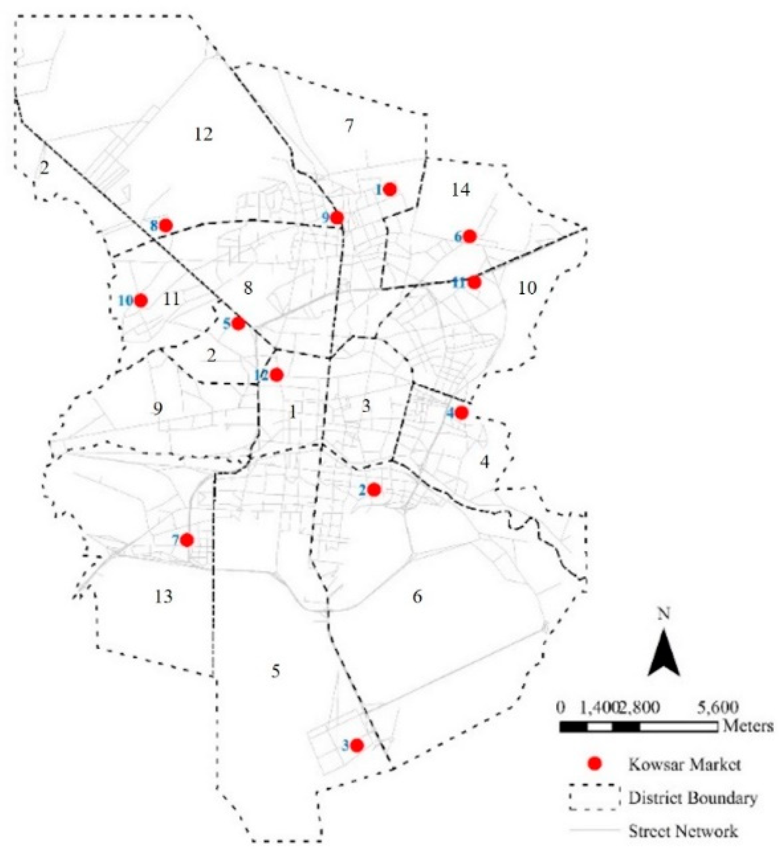
Access to high quality and healthy foods is crucial for city residents, particularly for low- and middle-income families. [68,76]. In this way, the municipality of Isfahan constructed 12 Kowsar discount retail markets to supply the needs of people in the city of Isfahan, Iran. In doing so, assessing the accessibility of TAZs of Isfahan was taken into account to test the applicability of the model in a real-world problem. Figure 1 depicts the study area along with distribution of the markets.
Briefly, inputs of the model are: (1) A trip chain showing the travel origin and destination (location of the fixed activities), (2) time budget, (3) on-time arrival probability for conducting the selected trip chain, (4) travel time of edges in the study area, and (5) area of the intermediate opportunities along with their locations. These items were set as below:
  • Trip chain H o m e Kowsar   m a r k e t H o m e was defined due to the portion of home-based trips among the other trips (about 90% of all trips).
  • Modeling period was considered the time window between 5:00 p.m. and 8:00 p.m., including the afternoon peak hour.
  • Time budget was set to 60 minutes, following previous studies [36].
  • Area of markets was considered as the indicator of opportunity attractiveness (Table 4).
  • On-time arrival probability was defined 99% for simulating extreme conditions, which gives minimum value or lower bound of accessibility.
  • Travel time distributions were set to normal, exponential, and log-normal distributions as travel time uncertainty in urban street networks is commonly defined by pre-allocated distributions [62]. Normal distribution was selected to provide a ground for comparing the results of the non-normal model with the conventional outputs. Additionally, log-normal distribution was taken into account because this distribution could model travel time in a more realistic manner [77].
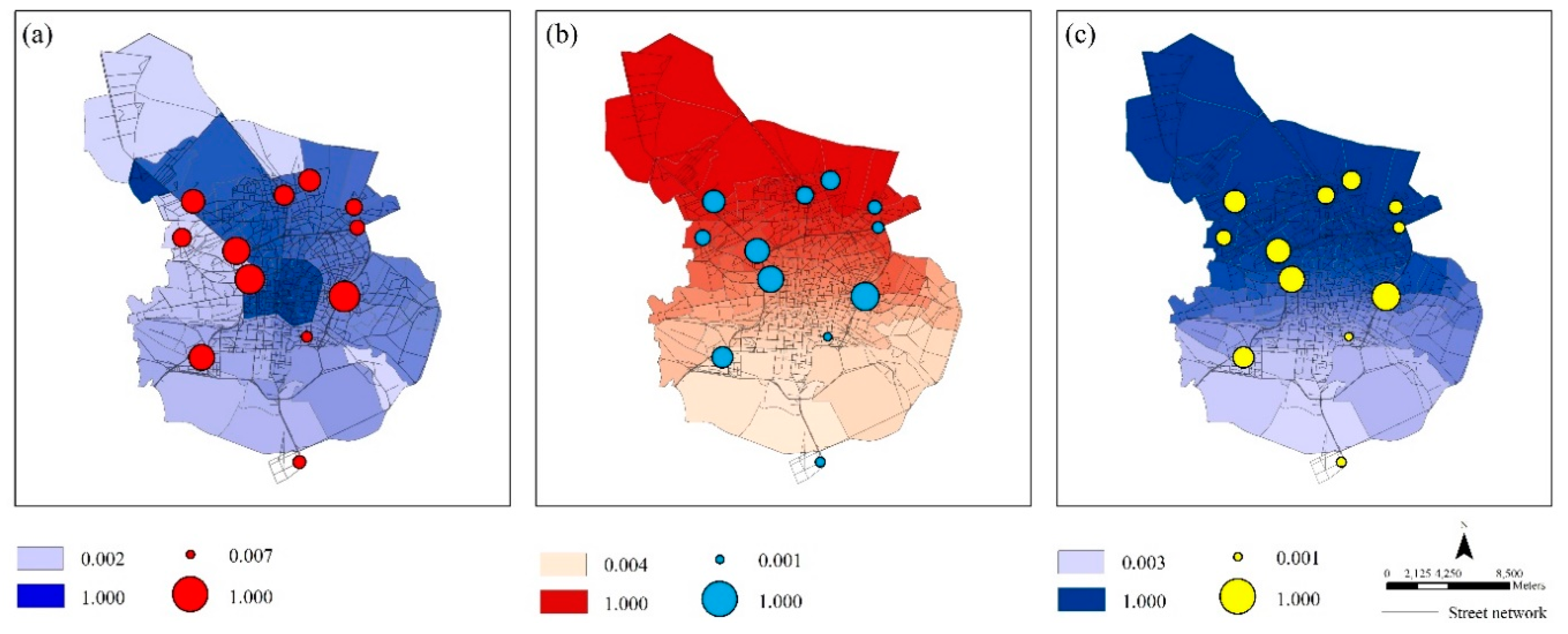
To construct NNRNTP, normal reliable NTP (NRNTP), and measure accessibility of TAZs to Kowsar markets, algorithms given in the previous section were implemented using MATLAB programming language. Results were visualized by ESRI ArcGIS, the main analytical software in transportation (GIS-T) and urban planning. Figure 2 illustrates the accessibility level of each market and the accessibility of TAZs.
A t-test was performed on the outputs to test the difference between accessibility of TAZs in normally and non-normally distributed networks. Generally, null and alternative hypothesizes of this test are equality and inequality of means between two groups, respectively. T-test checks whether the null or the alternative hypothesis could be rejected at a certain confidence interval. In addition, this test is used when the number of samples is more than 30. Thus, hypothesizes of this test for analyzing accessibility in the study area are elaborated as below:
  • Null hypothesis ( H 0 ): There is no statistically meaningful difference between the average of TAZ accessibility values in normally and non-normally distributed networks.
  • Alternative hypothesis ( H 1 ): There is a statistically meaningful difference between the average of TAZ accessibility values in normally and non-normally distributed networks.
The results of this test confirmed the difference between accessibility level of TAZs in normally and non-normally distributed networks (Table 5).
Moreover, to examine the difference between NNRNTP and NRNTP, size of constructed space-time prisms for each TAZ was recorded and compared using a t-test. Prism size is the area of space-time polygons calculated by Equation (2) for each edge in the potential path area. Table 6 presents the results of the t-test. It shows a meaningful difference between the size of NNRNTPs and NRNTP.
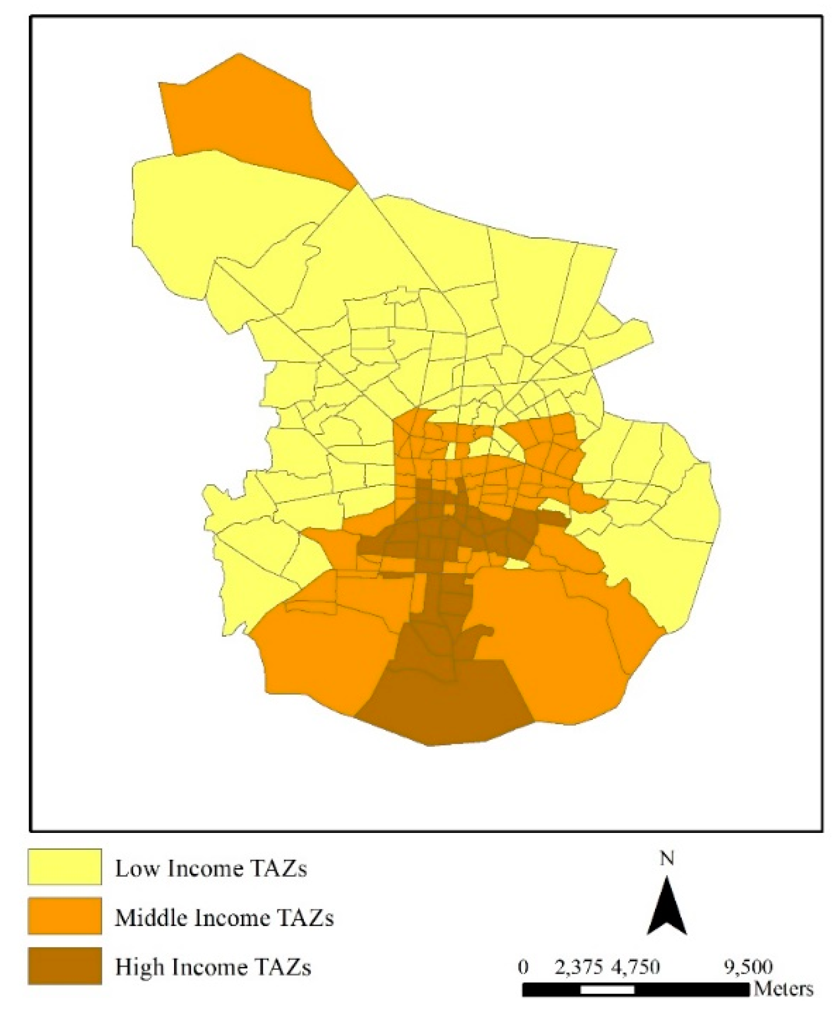
Moreover, it could be observed that northern TAZs had larger access to the markets than the southern ones. In addition, comparing accessibility values achieved by NNRNTPs with the income of people living in TAZs portrayed that low-income TAZs had larger values than the others (Figure 3).

4. Summary and Conclusion

In this study, a model was developed for quantifying accessibility to urban opportunities. This model incorporates network-based space-time prisms that could be implemented on stochastic networks with non-normal travel time distributions.
Firstly, a computational method was introduced for calculating reliable space-time prisms under the aforementioned conditions. Secondly, an accessibility measure was elaborated by combining the proposed space-time prism with the magnitude of urban opportunities. Finally, the accessibility model was applied in a study area under the extreme condition illustrating the lower bound of accessibility level regarding normal, exponential, and log-normal distributions.
Results demonstrated the applicability of the proposed model and statistical meaningfulness of difference between outputs of normal and non-normal methods. Results also illustrated the distribution of accessibility throughout the city of Isfahan where northern TAZs had larger access to the markets in comparison with southern ones.
For future studies, application of the introduced model in other cases for analyzing different urban phenomena is recommended. Another extension to this research is considering the correlation between link travel times in urban networks and modeling this effect in the structure of space-time prisms and accessibility metrics.

Author Contributions

Conceptualization, A.S. and M.M. and H.H; Methodology, A.S.; Programming of the algorithms, A.S.; Supervision, M.M. and H.H.; Writing – original draft, A.S.; Writing – review & editing, A.S.

Funding

This research received no external funding.

Conflicts of Interest

The authors declare no conflict of interest.

Appendix A. Classical Network-Based Space-Time Prisms

Equations for constructing conventional space-time prisms are presented below, where P P A is potential path area, t R N r x is time of the shortest path from origin r to x , t R N x s is time of the shortest path from x to destination s , b is time budget, F C is the set of places reachable from origin at t , B C is the set of places that can access destination during t , and N T P is network-based space-time prism.
P P A = { x | t R N r x + t R N x s b }
F C ( t ) = { x | t R N r x t t r   t t s }
B C ( t ) = { x | t R N x s t s t   t t r }
N T P ( t ) = F C ( t ) B C ( t )

References

  1. Geurs, K.T.; Ritsema van Eck, J. Accessibility Measures: Review and Applications. Evaluation of Accessibility Impacts of Land-Use Transportation Scenarios, and Related Social and Economic Impact; RIVM rapport 408505006; RIVM: Bilthoven, The Netherlands, 2001. [Google Scholar]
  2. Geurs, K.T.; Van Wee, B. Accessibility evaluation of land-use and transport strategies: Review and research directions. J. Transp. Geogr. 2004, 12, 127–140. [Google Scholar] [CrossRef]
  3. Hansen, W.G. How accessibility shapes land use. J. Am. Inst. Plan. 1959, 25, 73–76. [Google Scholar] [CrossRef]
  4. Ingram, D.R. The concept of accessibility: A search for an operational form. Reg. Stud. 1971, 5, 101–107. [Google Scholar] [CrossRef]
  5. Cascetta, E.; Cartenì, A.; Montanino, M. A new measure of accessibility based on perceived opportunities. Procedia Soc. Behav. Sci. 2013, 87, 117–132. [Google Scholar] [CrossRef]
  6. Banister, D. The sustainable mobility paradigm. Transport Policy 2008, 15, 73–80. [Google Scholar] [CrossRef]
  7. Ferreira, A.; Beukers, E.; Te Brömmelstroet, M. Accessibility is gold, mobility is not: A proposal for the improvement of Dutch transport-related cost-benefit analysis. Environ. Plan. B Plan. Des. 2012, 39, 683–697. [Google Scholar]
  8. Handy, S.L. Accessibility-vs. Mobility-Enhancing Strategies for Addressing Automobile Dependence in the US; Institute of Transportation Studies: Davis, CA, USA, 2002. [Google Scholar]
  9. Song, Y. Green Accessibility: Estimating the Environmental Costs of Space-Time Prisms for Sustainable Transportation Planning. Ph.D. Thesis, The Ohio State University, Columbus, OH, USA, 2015. [Google Scholar]
  10. Wang, Y.; Monzon, A.; Di Ciommo, F. Assessing the accessibility impact of transport policy by a land-use and transport interaction model—The case of Madrid. Comput. Environ. Urban Syst. 2015, 49, 126–135. [Google Scholar] [CrossRef]
  11. Liao, F.; van Wee, B. Accessibility measures for robustness of the transport system. Transportation 2016, 44, 1213–1233. [Google Scholar] [CrossRef] [Green Version]
  12. Bocarejo, S.J.P.; Oviedo, H.D.R. Transport accessibility and social inequities: A tool for identification of mobility needs and evaluation of transport investments. J. Transp. Geogr. 2012, 24, 142–154. [Google Scholar] [CrossRef]
  13. Kim, H.-M. Gender and Individual Space-Time Accessibility: A Gis-Based Geocomputational Approach. Ph.D. Thesis, The Ohio State University, Columbus, OH, USA, 2005. [Google Scholar]
  14. Kim, H.-M.; Kwan, M.-P. Space-time accessibility measures: A geocomputational algorithm with a focus on the feasible opportunity set and possible activity duration. J. Geogr. Syst. 2003, 5, 71–91. [Google Scholar] [CrossRef]
  15. Scott, D.; Horner, M. Examining the role of urban form in shaping people’s accessibility to opportunities: An exploratory spatial data analysis. J. Transp. Land Use 2008, 1, 89–119. [Google Scholar]
  16. Merlin, L.A. Accessibility, Travel Behavior, and Urban Form Change. Ph.D. Thesis, The University of North Carolina at Chapel Hill, Chapel Hill, NC, USA, 2014. [Google Scholar]
  17. Song, Y.; Miller, H.J.; Zhou, X.; Proffitt, D. Modeling Visit Probabilities within Network-Time Prisms Using Markov Techniques. Geogr. Anal. 2016, 48, 18–42. [Google Scholar] [CrossRef]
  18. Cimaroli, K.; Páez, A.; Newbold, K.B.; Heddle, N.M. Individual and contextual determinants of blood donation frequency with a focus on clinic accessibility: A case study of Toronto, Canada. Health Place 2012, 18, 424–433. [Google Scholar] [CrossRef] [PubMed]
  19. Horner, M.W.; Mascarenhas, A.K. Analyzing location-based accessibility to dental services: An Ohio case study. J. Public Health Dent. 2007, 67, 113–118. [Google Scholar] [CrossRef] [PubMed]
  20. Malekzadeh, A. Measurement of Transit Network Accessibility Based on Access Stop Choice Behaviour. Ph.D. Thesis, Queensland University of Technology, Brisbane, Australia, 2015. [Google Scholar]
  21. Baradaran, S.; Ramjerdi, F. Performance of accessibility measures in Europe. J.Transp. Stat. 2001, 4, 31–48. [Google Scholar]
  22. Bhat, C.R. Development of an Urban Accessibility Index: Literature Review; Center for Transportation Research, Bureau of Engineering Research, The University of Texas at Austin: Austin, TX, USA, 2000. [Google Scholar]
  23. Curtis, C.; Scheurer, J. Planning for sustainable accessibility: Developing tools to aid discussion and decision-making. Prog. Plan. 2010, 74, 53–106. [Google Scholar] [CrossRef]
  24. Breheny, M.J. The measurement of spatial opportunity in strategic planning. Reg. Stud. 1978, 12, 463–479. [Google Scholar] [CrossRef]
  25. Envall, P. Accessibility Planning: A Chimera? Ph.D. Thesis, University of Leeds, Leeds, UK, 2007. [Google Scholar]
  26. Chen, A.; Yang, C.; Kongsomsaksakul, S.; Lee, M. Network-based accessibility measures for vulnerability analysis of degradable transportation networks. Netw. Spat. Econ. 2007, 7, 241–256. [Google Scholar] [CrossRef]
  27. Dong, X.; Ben-Akiva, M.E.; Bowman, J.L.; Walker, J.L. Moving from trip-based to activity-based measures of accessibility. Transp. Res. Part A Policy Pract. 2006, 40, 163–180. [Google Scholar] [CrossRef]
  28. El-Geneidy, A.M.; Levinson, D.M. Access to destinations: Development of accessibility measures. Available online: https://conservancy.umn.edu/handle/11299/638 (accessed on 9 September 2019).
  29. Makri, M.-C.; Folkesson, C. Accessibility Measures for Analyses of Land Use and Travelling with Geographical Information Systems; Department of Technology and Society, Lund Institute of Technology: Lund, Sweden, 1999; pp. 1–17. [Google Scholar]
  30. Knox, P.L. The intraurban ecology of primary medical care: Patterns of accessibility and their policy implications. Environ. Plan. A 1978, 10, 415–435. [Google Scholar] [CrossRef]
  31. Van Wee, B.; Hagoort, M.; Annema, J.A. Accessibility measures with competition. J. Transp. Geogr. 2001, 9, 199–208. [Google Scholar] [CrossRef]
  32. Weibull, J.W. An axiomatic approach to the measurement of accessibility. Reg. Sci. Urban Econ. 1976, 6, 357–379. [Google Scholar] [CrossRef]
  33. Shen, Q. Location characteristics of inner-city neighborhoods and employment accessibility of low-wage workers. Environ. Plan. B Plan. Des. 1998, 25, 345–365. [Google Scholar] [CrossRef]
  34. Wilson, A.G. A family of spatial interaction models, and associated developments. Environ. Plan. A 1971, 3, 1–32. [Google Scholar] [CrossRef]
  35. Cascetta, E.; Cartenì, A.; Montanino, M. A behavioral model of accessibility based on the number of available opportunities. J. Transp. Geogr. 2016, 51, 45–58. [Google Scholar] [CrossRef]
  36. Chen, B.Y.; Yuan, H.; Li, Q.; Wang, D.; Shaw, S.-L.; Chen, H.-P.; Lam, W.H. Measuring place-based accessibility under travel time uncertainty. Int. J. Geogr. Inf. Sci. 2016, 31, 1–22. [Google Scholar] [CrossRef]
  37. Miller, H. Place-based versus people-based geographic information science. Geogr. Compass 2007, 1, 503–535. [Google Scholar] [CrossRef]
  38. Ettema, D.; Timmermans, H. Space-time accessibility under conditions of uncertain travel times: Theory and numerical simulations. Geogr. Anal. 2007, 39, 217–240. [Google Scholar] [CrossRef]
  39. Ben-Akiva, M.; Lerman, S.R. Disaggregate travel and mobility choice models and measures of accessibility. Behav. Travel Model. 1979, 654–679. [Google Scholar]
  40. Ben-Akiva, M.E.; Lerman, S.R. Discrete Choice Analysis: Theory and Application to tRavel Demand; MIT Press: Cambridge, MA, USA, 1985; Volume 9. [Google Scholar]
  41. Miller, H.J.; Wu, Y.-H. GIS software for measuring space-time accessibility in transportation planning and analysis. GeoInformatica 2000, 4, 141–159. [Google Scholar] [CrossRef]
  42. Hägerstraand, T. What about people in regional science? Pap. Reg. Sci. 1970, 24, 7–24. [Google Scholar] [CrossRef]
  43. Lenntorp, B. Paths in space-time environments: A time-geographic study of movement possibilities of individuals. Environ. Plan. A 1977, 9, 961–972. [Google Scholar]
  44. Cerdá, A. Accessibility: A Performance Measure for Land-Use and Transportation Planning in the Montréal Metropolitan Region; Supervised Research Project Report; School of Urban Planning McGill University: Montreal, QC, Canada, 2009. [Google Scholar]
  45. Kwan, M.-P.; Weber, J. Scale and accessibility: Implications for the analysis of land use–travel interaction. Appl. Geogr. 2008, 28, 110–123. [Google Scholar] [CrossRef]
  46. Miller, H.J. Modelling accessibility using space-time prism concepts within geographical information systems. Int. J. Geogr. Inf. Syst. 1991, 5, 287–301. [Google Scholar] [CrossRef]
  47. Miller, H.J. Measuring space-time accessibility benefits within transportation networks: Basic theory and computational procedures. Geogr. Anal. 1999, 31, 1–26. [Google Scholar] [CrossRef]
  48. Miller, H.J.; Bridwell, S.A. A field-based theory for time geography. Ann. Assoc. Am. Geogr. 2009, 99, 49–75. [Google Scholar] [CrossRef]
  49. Song, Y.; Miller, H.J. Simulating visit probability distributions within planar space-time prisms. Int. J. Geogr. Inf. Sci. 2014, 28, 104–125. [Google Scholar] [CrossRef]
  50. Kwan, M.P. Space-time and integral measures of individual accessibility: A comparative analysis using a point-based framework. Geogr. Anal. 1998, 30, 191–216. [Google Scholar] [CrossRef]
  51. Li, Q.; Zhang, T.; Wang, H.; Zeng, Z. Dynamic accessibility mapping using floating car data: A network-constrained density estimation approach. J. Transp. Geogr. 2011, 19, 379–393. [Google Scholar] [CrossRef]
  52. Neutens, T.; Schwanen, T.; Witlox, F.; De Maeyer, P. Equity of urban service delivery: A comparison of different accessibility measures. Environ. Plan. A 2010, 42, 1613–1635. [Google Scholar] [CrossRef]
  53. Du, L.; Peeta, S.; Kim, Y.H. An adaptive information fusion model to predict the short-term link travel time distribution in dynamic traffic networks. Transp. Res. Part B Methodol. 2012, 46, 235–252. [Google Scholar] [CrossRef]
  54. Lam, W.H.; Shao, H.; Sumalee, A. Modeling impacts of adverse weather conditions on a road network with uncertainties in demand and supply. Transp. Res. Part B Methodol. 2008, 42, 890–910. [Google Scholar] [CrossRef]
  55. Kuijpers, B.; Miller, H.J.; Neutens, T.; Othman, W. Anchor uncertainty and space-time prisms on road networks. Int. J. Geogr. Inf. Sci. 2010, 24, 1223–1248. [Google Scholar] [CrossRef]
  56. Kobayashi, T.; Miller, H.J.; Othman, W. Analytical methods for error propagation in planar space-time prisms. J. Geogr. Syst. 2011, 13, 327–354. [Google Scholar] [CrossRef]
  57. Liao, F.; Rasouli, S.; Timmermans, H. Incorporating activity-travel time uncertainty and stochastic space-time prisms in multistate supernetworks for activity-travel scheduling. Int. J. Geogr. Inf. Sci. 2014, 28, 928–945. [Google Scholar] [CrossRef]
  58. Chen, B.Y.; Li, Q.; Wang, D.; Shaw, S.-L.; Lam, W.H.; Yuan, H.; Fang, Z. Reliable space-time prisms under travel time uncertainty. Ann. Assoc. Am. Geogr. 2013, 103, 1502–1521. [Google Scholar] [CrossRef]
  59. de Palma, A.; Picard, N. Route choice decision under travel time uncertainty. Transp. Res. Part A Policy Pract. 2005, 39, 295–324. [Google Scholar] [CrossRef]
  60. Lam, T.C.; Small, K.A. The value of time and reliability: Measurement from a value pricing experiment. Transp. Res. Part E Logist. Transp. Rev. 2001, 37, 231–251. [Google Scholar] [CrossRef]
  61. Chen, B.Y.; Lam, W.H.; Sumalee, A.; Li, Q.; Shao, H.; Fang, Z. Finding reliable shortest paths in road networks under uncertainty. Netw. Spat. Econ. 2013, 13, 123–148. [Google Scholar] [CrossRef]
  62. Ji, Z.; Kim, Y.S.; Chen, A. Multi-objective α-reliable path finding in stochastic networks with correlated link costs: A simulation-based multi-objective genetic algorithm approach (SMOGA). Expert Syst. Appl. 2011, 38, 1515–1528. [Google Scholar] [CrossRef]
  63. van Wee, B. Viewpoint: Toward a new generation of land use transport interaction models. J. Transp. Land Use 2015, 8, 1–10. [Google Scholar]
  64. van Wee, B. Accessible accessibility research challenges. J. Transp. Geogr. 2016, 51, 9–16. [Google Scholar] [CrossRef]
  65. Geertman, S.C.; Ritsema Van Eck, J.R. GIS and models of accessibility potential: An application in planning. Int. J. Geogr. Inf. Syst. 1995, 9, 67–80. [Google Scholar] [CrossRef]
  66. Hillsdon, M.; Panter, J.; Foster, C.; Jones, A. The relationship between access and quality of urban green space with population physical activity. Public Health 2006, 120, 1127–1132. [Google Scholar] [CrossRef] [PubMed]
  67. Huang, L.; Li, Q.; Yue, Y. Activity identification from GPS trajectories using spatial temporal POIs’ attractiveness. In Proceedings of the 2nd ACM SIGSPATIAL International Workshop on Location Based Social Networks, San Jose, CA, USA, 2 November 2010; pp. 27–30. [Google Scholar]
  68. Sahebgharani, A.; Haghshenas, H.; Mohammadi, M. A Markovian Measure for Evaluating Accessibility to Urban Opportunities. J. Transp. Land Use 2019, 12, 19–43. [Google Scholar] [CrossRef]
  69. Wu, Y.-H.; Miller, H.J. Computational tools for measuring space-time accessibility within transportation networks with dynamic flow. J. Transp. Stat. 2001, 4, 1–14. [Google Scholar]
  70. Gutiérrez, E.; Medaglia, A.L. Labeling algorithm for the shortest path problem with turn prohibitions with application to large-scale road networks. Ann. Oper. Res. 2008, 157, 169–182. [Google Scholar] [CrossRef]
  71. Der Kiureghian, A.; Liu, P.-L. Structural reliability under incomplete probability information. J. Eng. Mech. 1986, 112, 85–104. [Google Scholar] [CrossRef]
  72. Liao, F.; Arentze, T.; Timmermans, H. Incorporating space-time constraints and activity-travel time profiles in a multi-state supernetwork approach to individual activity-travel scheduling. Transp. Res. Part B Methodol. 2013, 55, 41–58. [Google Scholar] [CrossRef]
  73. Robert, C.P. Monte Carlo Methods; Wiley Online Library: Hoboken, NJ, USA, 2004. [Google Scholar]
  74. Horner, M.W.; Downs, J. Integrating people and place: A density-based measure for assessing accessibility to opportunities. J. Transp. Land Use 2014, 7, 23–40. [Google Scholar] [CrossRef] [Green Version]
  75. Lee, B.H.; Waddell, P.; Wang, L.; Pendyala, R.M. Operationalizing Time-Space Prism Accessibility in a Building-Level Residential Choice Model. In Proceedings of the 88th Annual Meeting of the TRB, Washington, DC, USA, 11–15 January 2019. [Google Scholar]
  76. Widener, M.J.; Farber, S.; Neutens, T.; Horner, M.W. Using urban commuting data to calculate a spatiotemporal accessibility measure for food environment studies. Health Place 2013, 21, 1–9. [Google Scholar] [CrossRef] [PubMed] [Green Version]
  77. Srinivasan, K.K.; Prakash, A.; Seshadri, R. Finding most reliable paths on networks with correlated and shifted log–normal travel times. Transp. Res. Part B Methodol. 2014, 66, 110–128. [Google Scholar] [CrossRef]
Figure 1. Study area.
Computation 07 00051 g001
Figure 2. Accessibility of markets and traffic analysis zones (TAZs) (normalized values). (a) Accessibility with normal reliable space-time prism (NRNTP). (b) Accessibility with exponential non-normal reliable space-time prism (NNRNTP). (c) Accessibility with log-normal NNRNTP.
Computation 07 00051 g002
Figure 3. Income distribution in the city of Isfahan.
Computation 07 00051 g003
Table 1. Parameters used in model development.
SymbolDefinition
r Index of trip origin, r V
s Index of trip destination, s V
t r Departure time from origin ( r )
t s Arrival time to destination ( s )
b Travel time budget ( b = t s t r )
Q Set of individuals or set of population groups
q Index of an individual or a population group
α On-time arrival probability depicting risk-taking behavior of a traveler
α q On-time arrival probability of individual or population group q Q
t i a The earliest arrival time to vertex i V
t i b The latest departure time from vertex i V
x i x co-ordinate of vertex i V
y i y co-ordinate of vertex i V
K Set of all intermediate opportunities or points of interest k
Z Set of traffic analysis zones (TAZs) in a geographic area
z , z ´ Indices of TAZs
C I Set of confidence interval including α n
P z Population of TAZ z Z
P ´ z α q Portion of population group q in TAZ z conducting their trip at confidence interval α q
O k Attractiveness of opportunity k K . Area could represent attractiveness of an opportunity [65,66,67,68,69].
O m a x Maximum attractiveness of opportunities, max k K ( O k )
B ( k ) A binary variable with value of 1 if activity k be in space-time prism, and 0 otherwise.
L i j Set of paths start from vertex i V and end to vertex j V
L w i j Set of paths from vertex w V to vertex j V passing through edge e i j
u Index of a path in L or L w i j
l u i j Path u L i j from vertex i V to vertex j V
l u w i j Path u L w i j from vertex w V to vertex j V passing through edge e i j
l N D M i j Non-dominated path from vertex i V to vertex j V
l N D M r i j Non-dominated path from vertex w V to vertex j V passing through edge e i j
F l u i j 1 ( α ) Value of inverse cumulative density function of l u i j at confidence interval α
Table 2. Distribution parameters.
EdgeFirst ParameterSecond Parameter
U157
U21011
U31513
U41820
U546
Table 3. Result of Monte Carlo Simulation for the given example (The highlighted cell is travel time of the path at confidence interval 80%).
Random Samples Taken from Distributions in Table 2SummationSorting
U1U2U3U4U5
6.28410.62013.84719.0585.04954.86052.477
5.44210.60013.37819.6595.94555.02653.748
6.67410.17214.19219.7175.42056.17754.257
6.94210.09013.02319.5784.62354.25754.860
6.69210.25514.82018.6354.58254.98654.986
6.01110.85814.35818.9045.70055.83355.026
5.55710.91113.97719.5045.82355.77355.569
6.49310.69914.87818.2195.27855.56955.773
5.47310.72513.54818.2194.51052.47755.833
6.91410.22913.88618.5394.17753.74856.177
Table 4. Attractiveness of Kowsar markets (standardized values).
Opportunity_ID123456789101112
Attractiveness0.370.090.1810.330.020.540.650.260.280.200.48
Table 5. t-test for analyzing the difference between the accessibility of TAZs generated by the models.
t-test in 95% of Confidence Interval for Accessibility Value of TAZs
Distribution typeAccessibility with exponential NNRNTPAccessibility with log-normal NNRNTP
t valueSig. (2-tailed)t valueSig. (2-tailed)
Accessibility with NRNTP8.3540.0006.2540.000
Accessibility with log-normal NNRNTP−7.9380.000--
Table 6. t-test for analyzing the difference between the size of NNRNTP and NRNTP.
t-test in 95% of confidence interval
Size of NNRNTP with exponential distributionSize of NNRNTP with log-normal distribution
t valueSig. (2-tailed)t valueSig. (2-tailed)
Size of NRNTP3.2330.0037.0850.000

