Modeling and Analysis of Autonomous Agents’ Decisions in Learning to Cross a Cellular Automaton-Based Highway

Abstract

For a better understanding of the nature of complex systems modeling, computer simulations and the analysis of the resulting data are major tools which can be applied. In this paper, we study a statistical modeling problem of data coming from a simulation model that investigates the correctness of autonomous agents’ decisions in learning to cross a cellular automaton-based highway. The goal is a better understanding of cognitive agents’ performance in learning to cross a cellular automaton-based highway with different traffic density. We investigate the effects of parameters’ values of the simulation model (e.g., knowledge base transfer, car creation probability, agents’ fear and desire to cross the highway) and their interactions on cognitive agents’ decisions (i.e., correct crossing decisions, incorrect crossing decisions, correct waiting decisions, and incorrect waiting decisions). We firstly utilize canonical correlation analysis (CCA) to see if all the considered parameters’ values and decision types are significantly statistically correlated, so that no considered dependent variables or independent variables (i.e., decision types and configuration parameters, respectively) can be omitted from the simulation model in potential future studies. After CCA, we then use the regression tree method to explore the effects of model configuration parameters’ values on the agents’ decisions. In particular, we focus on the discussion of the effects of the knowledge base transfer, which is a key factor in the investigation on how accumulated knowledge/information about the agents’ performance in one traffic environment affects the agents’ learning outcomes in another traffic environment. This factor affects the cognitive agents’ decision-making abilities in a major way in a new traffic environment where the cognitive agents start learning from existing accumulated knowledge/information about their performance in an environment with different traffic density. The obtained results provide us with a better understanding of how cognitive agents learn to cross the highway, i.e., how the knowledge base transfer as a factor affects the experimental outcomes. Furthermore, the proposed methodology can become useful in modeling and analyzing data coming from other computer simulation models and can provide an approach for better understanding a factor or treatment effect.

1. Introduction

Artificial intelligence and machine learning techniques are now widely used in the analysis of many real-world complex systems coming from manufacturing, business, information technology, and engineering, to name a few among many others [1,2,3]. They are important techniques that aim at capturing key data patterns [4,5]. From the theoretical perspective, it is a fundamental problem to understand how the response variables of a complex system change when the input conditions and values of independent variables/factors change [6,7]. If a research study is observational, answering this question is difficult and, in fact, almost impossible due to lack of cause-and-effect relationships between the response variables and the factors that are used for describing the responses [8]. The observational study can tell if there are some associations between response variables and predictor variables. If yes, one can only be able to conclude that predictor variables are useful and are able to contribute the explanations of data variation of the response variables. Therefore, data obtained from the real-world observational study is not able to provide us with the causal inference for the regression model that is used for describing the response variables [8]. Because of this, to be able to better understand the nature of complex systems, a computer simulation of complex systems becomes an important approach. This is due to its capability of justifying the cause-and-effect relationships between the response variables and input configuration parameters values. Most of the real-word information applications are complex systems [9,10,11]. For example, robots are complex systems that involve complicated software and hardware systems, as well as interactive information processing [12]. Intelligent robots are expected to be able to improve their ability by self-learning from past experiences. The entire process of improvement of an intelligent robot is exactly the application of machine learning techniques, such as feature extraction, feature selection, and neural networks [13,14]. To carry out some tasks (e.g., exploration of unknown space), it is more efficient and reliable to employ swarm of simple robots instead of employing one complex robot, as a swarm of robots can accomplish the task faster and more effectively even if some robots break [14,15]. The small and simple robots cost less to be produced, and the maintenance cost is much lower than the cost of a complex robot. Another example is the risk appetite of investors in stock markets. When stock prices go up or down, investors must decide either to buy more or to sell more or to do nothing and wait until next time. The investing behavior can be complex, and knowing how investment decisions are related to the risk appetite could be important for a better understanding of the dynamics of financial markets.

All of these factors motivated us to conduct a simulation study of cognitive agents learning to cross a cellular automaton-based highway, developed by Lawniczak, Di Stefano, Ernst, and Yu [16,17,18,19,20,21,22] and its modeling problem of the data coming from the simulation. Within this modeling and simulation study, the cognitive agents are abstractions of simple robots, which are generated at a crossing point of the highway. The sole goal of the agents is to learn to cross the road successfully through vehicle traffic. The agents can share and update their knowledge about their previous performance in carrying the task of crossing the unidirectional single lane road. Through the learning process, they can make more sensible decisions to cross or to wait, so that the successful crossing rates or successful waiting rates are improved. This is very much like the situation when an autonomous vehicle is waiting at the edge of a country highway and it is trying to make a left turn. A country highway is often bi-directional and has only a single lane in each direction. When crossing to make a left turn, to avoid being hit by an incoming vehicle, the autonomous vehicle must decide, sequentially at each given time step, according to the traffic conditions, on either continuing to wait or making a left turn. This simulation study and its analysis can help us better understand the effects of various experimental conditions on the experimental outcomes such as successful crossing. Because of the similarity between the decision-making of cognitive agents in our simulation and an autonomous vehicle decision-making in an actual situation, the research outcomes eventually may contribute to better understanding of how to improve the performance of autonomous vehicles’ decision-making process. Also, for the financial market example mentioned earlier, this study may help to provide a guide for understanding the effect of different levels of risk appetite on the investment decision-making.

When simulating the experiment of cognitive agents learning to cross a highway, the agents’ crossing behavior will depend on the set-ups of the configuration parameters’ values in the simulation, such as a value of car creation probability, or the values of agents’ fear and desire to cross the highway. The different combinations of the parameters’ values can lead to the different outcomes (e.g., success or failure) of the agents’ crossing or waiting decisions. Thus, it is important to investigate the cause-and-effect relationships among these factors and the decision types, and to study how much the main factors can contribute to the regression model that is used to capture such relationships. Due to this expectation of our study, we firstly applied canonical correlation analysis (CCA) to investigate the correlation between the combined configuration parameters’ values and the combined decisions, which are all linear combinations of either configuration parameters’ values or decision types. From the computational point of view, CCA maps the original data to canonical variate space, in which the potential association between the canonical variates can be discovered. On the one hand, it helps to reduce the data dimension, which is particularly important when the number of output response variables or the number of predictors is large. On the other hand, it justifies the use of statistical modeling techniques in the further analysis. From the methodological perspective, CCA is related to principal component analysis (PCA) and factor analysis (FA). The major difference is that CCA is applied to both, i.e., response variables and predictors, while PCA or FA is applied only to one set of variables, either response variables or predictor variables. However, it is not applied to both at the same time. The similarity among them is that they intend to transform the original data to the feature subspace, with the potential of having dimension reduction, so that the interpretation of data becomes easier. Since we tried to investigate the association between two set of variables, CCA became a better choice in this regard.

The objective of CCA is to maximize the canonical correlation between two variable sets, and then to produce a set of canonical variates that may be used to replace original variables when capturing correlations [23]. A more thorough study of the use of CCA allows us to reduce the dimension of the data frame while preserving the main effects of the relationships. It also allows us to find out which configuration of parameters’ values may influence the cognitive agents’ decisions the most. CCA is widely used in various areas. For example, in the field of economics, by constructing a CCA model for the Zimbabwe stock exchange, the impact of macroeconomic variables on stock returns could be verified [24]; in the field of biology, this method was promising in investigating the multivariate correlation between impulsivity and psychopathy [25]; in machine learning, the CCA method was applied to map the representation of biological images from the extracted features from extreme machine learning to a new feature space, which was used to reconstruct the biological images [26]. In brain–computer interfaces (BCIs), canonical correlation analysis was used to study the visual evoked potential for steady-state targets [27]. In this work, CCA is applied in a novel way to a simulation study to validate the cause-and-effect relationship between multivariate dependent variables and multiple independent variables.

Our simulation model is a complicated fully discrete algorithmic mathematical model involving many elements, e.g., a cellular automaton (CA)-based highway, vehicular traffic, cognitive agents, decision-making formulas, and knowledge base, and it involves many different experimental set-ups of the parameters’ values. Thus, the output data from the simulation are extremely large, and it is difficult to fit the data to some standard statistical models that often require certain assumptions. Because of this, we use the regression tree modeling approach to explore how the configuration parameters’ values influence the agents' decision-making abilities in different traffic density, which is considered as one of the key factors affecting the decision outcomes. In statistics, a decision tree is a modern method in decision analysis for explorations of the data grouping. It can also be used to predict the values of the underlying response variable [28], which is often referred to as the regression tree approach. It is widely used in many different fields. In Reference [29], a methodological review of the classification and regression tree (CART) analysis was conducted to help researchers to familiarize with this method. In Reference [30], a logistic regression tree-based method was applied to American older adults to identify fall risk factors and interaction effects of those risk factors. In Reference [31], the regression tree method was used to predict the school absenteeism severity from various demographic and academic variables such as youth age and grade level, and to find the main factors that lead to the absence. In Reference [32], a coastal ecosystem was simulated to study the growth behavior of bivalve species, and the regression tree analysis was conducted to investigate the leading factors associated with the water conditions that promote the quality and growth rate of species the most. In Reference [33], a simulation model of a rat in an elevated plus-maze was constructed to measure the anxiety-like behavior. After the computational simulation, the dominant parameters were investigated to improve the model performance through the regression tree method. As an algorithm-based method, regression tree can be useful to explore the complex data characteristics. Also, this method does not require any model assumptions. Since we focus on predictive modeling to better understand the effects of the factors that we designed for our simulation models, this is a typical type ANOVA model. However, from our investigation (not presented in this paper), validation of the model assumption becomes a big concern when the ANOVA linear model is considered. This is because our response variable is the accumulated effect from a given stochastic process, and it is unlikely to follow some specific distribution [34]. This means that the assumption about our response variable as a random variable with an identical distribution is unrealistic. Because of this, it is more suitable to model our response variable using a distribution-free method. The decision-tree type of regression approach becomes a natural choice for this problem. These factors motivated us to apply the regression tree method in a novel way to our designed computer simulation experiment of cognitive agents learning to cross a CA-based highway.

The main contribution of this work is the proposed method that combines CCA and regression trees for analyzing data from a designed computer simulation experiment for a better understanding of the nature of a complex system. It provides a systematic solution on investigating the effect of input parameters’ values on its response variables, especially the effect coming from the knowledge base transfer on the decision outcomes. To the best of our knowledge, this is the first type of work that uses a CCA and regression tree approach in modeling computer simulation data. The proposed methodologies are also suitable for other designed experiments with a similar research objective.

This paper is organized as follows: in Section 2, we introduce the simulation model including the associated variables. We discuss the simulation process and describe the data used in this work. In Section 3, we discuss the methodologies, including canonical correlation analysis and regression tree methods, which are used for obtaining the results presented in this paper. In Section 4, the justification of statistically significant correlation between the designed configuration parameters’ values and agents’ decisions is reported, and the regression tree results obtained for all four types of considered decisions are analyzed. Finally, in Section 5, we conclude our findings and provide summary remarks and outline potential future work.

2. Simulation Model Description

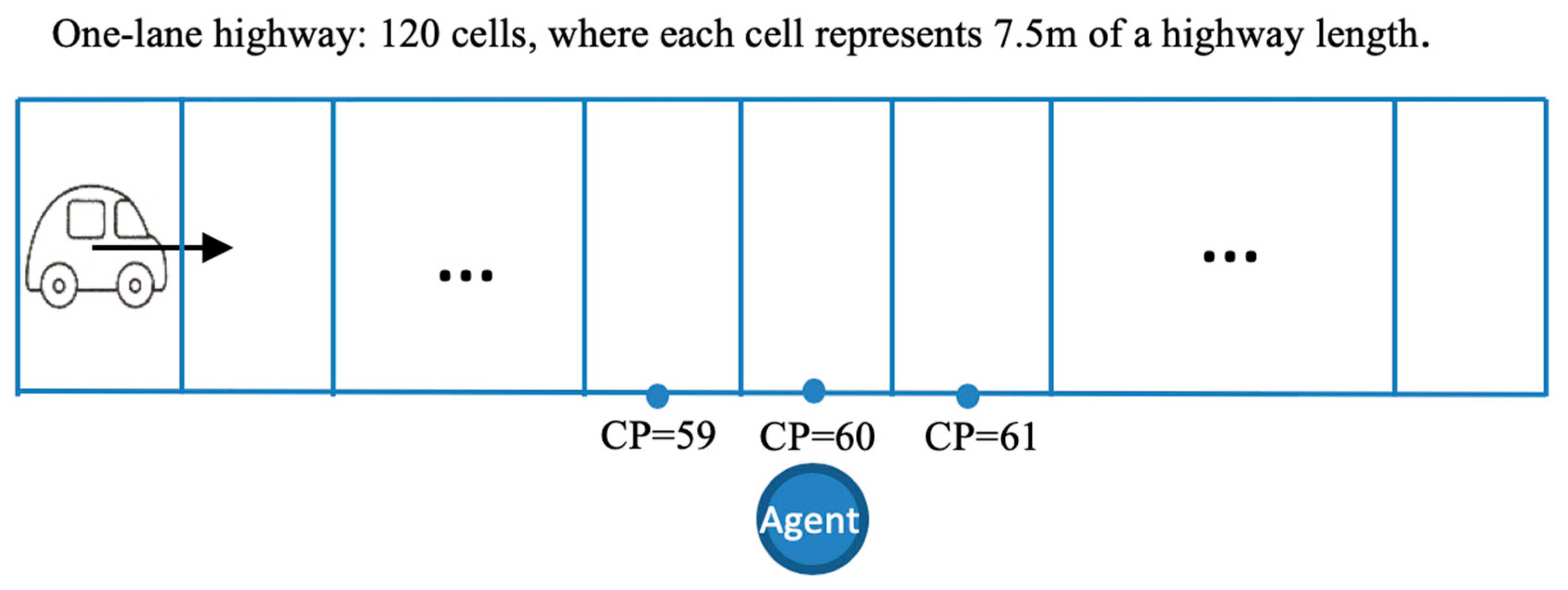
The model of autonomous agents’ learning to cross cellular automaton (CA)-based highway is a fully discrete algorithmic model, and it was developed by Lawniczak, Di Stefano, Ernst, and Yu [16,17,18,19,20,21,22]. It simulates the epitome of an actual vehicle driving and crossing environment and decision-making process through four main components: highway, vehicles, agents, and their decisions. In this paper, we provide a brief introduction to the model and its simulation process. The diagram of the abstraction of the highway, vehicles, and agents crossing the CA-based highway implemented in the model is displayed in Figure 1. For more information about the model description and previous statistical analysis of it simulation data, the reader is referred to References [16,17,18,19,20,21,22,35,36,37,38,39,40,41]. The highway and the vehicular traffic are modeled by the Nagel–Schreckenberg highway traffic model [42], which is a CA-based model consisting of a collection of cells, with each cell representing a segment of a highway of 7.5 m in length [42]. In our study, we consider a unidirectional one-lane highway composed of 120 cells. The vehicles move along the highway and the agents move across the highway. Thus, the state of each cell (i.e., empty or occupied) depends on whether a vehicle or an agent is present in a cell, and it is updated at each time step as the simulation progresses. Each car is randomly generated with speed 0 at the first cell of the highway at each time step. Once cars run on the highway, they follow the rules of the Nagel–Schreckenberg traffic model [42]. Notice that each car tries to reach its maximum speed set at software initialization, but to prevent a collision with another car, it adjusts its speed as required. However, it does not decelerate to avoid hitting an agent crossing the highway. There are two configuration parameters associated with the vehicle in the model, car creation probability and random deceleration. Car creation probability (CCP) is the probability that a vehicle is generated at the beginning of the highway, which simulates the density of traffic flow. Random deceleration (RD) controls the moving behaviors of the cars. It is a dummy variable that takes a value of either 0 or 1. If vehicles do not decelerate randomly as in the Nagel–Schreckenberg traffic model, then RD = 0; if the vehicles randomly and independently decelerate with the probability 0.5, as in the Nagel–Schreckenberg traffic model, then RD = 1.

The agents are an abstraction of autonomous robots. They aim at successfully crossing the highway without being hit by incoming cars. In the presented study, at each time step, an agent is generated at the selected crossing point (CP) on the same side of the highway. The CP at which agents are generated and placed in the queue, if there are other agents already waiting to cross the highway, is located at cell 60 (i.e., 450 m from the first cell), far away from the beginning of the highway, to allow emergence of the car traffic profiles typical for the considered CCP values. The agents have limited field of vision and they can perceive only fuzzy proximity values (e.g., close, medium, far) and fuzzy speed values (e.g., slow, medium fast, fast, very fast) of incoming cars. Two attributes are randomly and independently assigned to each agent: fear and desire. The values with which agents can experience fear and desire are set at the initialization of the software. Thus, the fear and desire can be interpreted as factors with various levels. Hence, the fear is the latent variable which measures an agent’s propensity to risk aversion in crossing the highway. The desire is the latent variable that measures an agent’s propensity to risk-taking in crossing the highway. The values of both fear and desire enter agents’ decision-making formulas, and they determine the value of the threshold with which an agent makes its decision to cross or not to cross the highway. If the decision-making formula tells an agent not to cross at its current location at a given time, depending on the initial set-up of the simulation software, the agent may move randomly with equal probability to one of the adjacent cells of its current CP location, or it may remain at its current CP. The agents’ ability to change their crossing points is governed by the horizontal movement (HM) factor. If HM = 0, then agents cannot change their CP set at the initialization at cell 60. If HM = 1, then each agent can change its crossing point by moving up to five cells away from CP = 60 in each direction. Thus, if HM = 1, then many more agents may simultaneously attempt to cross the highway, and agents may potentially attempt to cross from 11 crossing points.

An agent attempting to cross the highway is called an active agent, and it must make a decision that leads to one of the following decision outcomes: (1) correct crossing decision (CCD), an agent made a crossing decision and crossed successfully; (2) incorrect crossing decision (ICD), an agent made a crossing decision but it was hit by an incoming car; (3) correct waiting decision (CWD), an agent made a waiting decision, but if it decided to cross the highway, it would have been hit by an incoming car; (4) incorrect waiting decision (IWD), an agent made a waiting decision, but if it decided to cross the highway, it would have crossed successfully. The assessment of each active agent’s decision, i.e., if the decision was CCD, ICD, CWD, or IWD, is recorded as a count into the knowledge-based (KB) table of all the agents waiting at the crossing point of the active agent. Notice that, if HM = 1, then a KB table is associated with each crossing point and the values of its entries are used by active agents in the calculation of decision-making formula values when they are deciding what to do. Each knowledge-based table is organized as a matrix with the extra row entry reserved for out-of-range field-of-vision results. The columns of the KB table store information about qualitative descriptions of incoming cars velocities (i.e., slow, medium speed, fast, very fast) and the rows of the KB table store information about qualitative descriptions of the incoming cars proximities (i.e., close, medium far, far, and out of range). For details, see References [20,21,22]. In the presented simulation results, a car is perceived as close if it is 0–5 cells away, medium far if it is 6–10 cells away, far if it is 11–15 cells away, and out of range if it is 16 or more cells away, regardless of the velocity value of the car, and this is encoded in the extra entry of the KB table. A car is perceived as slow if its perceived velocity is 0–3 cells per time step, medium speed if its perceived velocity is 4–5 cells per time step, fast if its perceived velocity is 6–7 cells per time step, and very fast if its perceive velocity is 8–11 cells per time step. A car’s maximum speed can be 11 cells per time step.

At each time step, the KB table values provide cumulative information about the assessment of active agents’ decision type, from the beginning of each simulation run. The KB tables are updated at each simulation time step and, as time progresses, they accumulate more and more information about the active agents’ performance in their decision-making process. Thus, as time progresses, the active agents make their crossing and waiting decisions based on more information/knowledge about their performance in similar traffic conditions observed in the past. The decision-making formula they use is based on the observational social learning mechanism: “If this situation worked well for somebody else, it will probably work for me and, thus, I will imitate that somebody else. If this situation did not work well for somebody else, it will probably not work for me; thus, I will not imitate that somebody else.” [43]. Thus, using this observational social learning mechanism encoded into the agents decision-making formula and with the accumulation of information about their performance as time progresses, the agents learn how to cross the highway within each simulation run.

In the presented simulation model, in the first scenario (i.e., KBT = 0), each simulation run starts with the KB table initialized as tabula rasa, i.e., a “blank slate”, represented by “(0, 0, 0, 0)” at each table entry for the assumption that the active agents can cross for all possible (proximity, velocity) combinations. At the start of each simulation, active agents cross the highway regardless of the observed (proximity, velocity) combinations until the first successful crossing of an active agent or five (selected for the presented simulation results) consecutive unsuccessful crossings of the active agents, whichever comes first. This initial condition is introduced to more quickly populate the KB table entries. After the initialization of the simulation, for each observed (proximity, velocity) pair of an incoming car, each active agent consults the KB table to get information about agents’ performance in the past, to decide if it is safe or not to cross. Its decision is based on the implemented intelligence/decision-making formula, which for the observed (proximity, velocity) pair combines the success ratio of crossing the highway for this (proximity, velocity) pair with the active agent’s fear and/or desire parameters’ values, which determine that agent decision threshold value. Notice that, in the first scenario (i.e., KBT = 0), the active agents do not have any exiting knowledge/information about their performance when they start learning to cross the highway, and this knowledge/information is built only during each simulation run. Thus, it is interesting to investigate the active agents’ learning performance in crossing the highway if they have access to the information about agents’ performance in some other traffic environment, i.e., with some different CCP value. In the simulation model, this is incorporated through KB transfer. Thus, in the second scenario (i.e., KBT = 1), the KB table of the initial crossing point, CP = 60, is transferred at the end of a simulation run with a lower CCP value to the agents at the beginning of a simulation run with an immediately higher value of CCP. When KBT = 0, the KB tables are never transferred from agents in a traffic environment with a lower CCP value to the agents in an environment with an immediately higher CCP value or any other value. We considered the following CCP values in the presented simulations: 0.1, 0.3, 0.5, 0.7, and 0.9. When KBT = 1, each simulation in the traffic environment with CCP = 0.1 starts with the KB table tabula rasa, and the KB table built in this simulation run is transferred next to the agents at the beginning of the simulation run in the traffic environment with CCP = 0.3. This process of transferring the KB tables continues until the simulation starts in the traffic environment with CCP = 0.9, where the simulation with CCP = 0.9 starts with the KB table accumulated over the other four less dense traffic environments, i.e., with CCP = 0.1, 0.3, 0.5, and 0.7. This process of transferring KB tables is carried out for each simulation repeat when KBT = 1.

Given the above description of the model, the agents’ learning performance in crossing the highway is affected by the above-discussed model parameters, which are car creation probability (CCP), random deceleration (RD), agents’ fear and desire, horizontal movement (HM), and KB transfer (KBT). Therefore, we focus on studying the effects of these factors and their levels on the agents’ learning performance when they use a crossing-based decision formula (cDF) [20,21,22], which is described below.

After the initialization phase, at each time step t, each active agent, while deciding whether to cross or to wait, carries out several tasks: (1) it determines if there is a car in its horizon of vision; if yes, then it determines the fuzzy (i, j) values of the (proximity, velocity) pair for the current closest incoming car; (2) from the KB table associated with its CP, the active agent gets information about the number of CCDs and the number of ICDs for the observed (i, j) values of the (proximity, velocity) pair, or for the observed out-of-range vision situation, the entry of which is denoted by the (0,0) pair of indexes in the KB table; (3) for the observed (i, j) values of the (proximity, velocity) pair, the active agent calculates the value of the decision formula cDF, i.e., the value ${\mathrm{cDF}}_{\mathrm{ij}}\left(\mathrm{t}\right)$, corresponding to the (i, j) entry of the KB table (including the extra row entry). The expression ${\mathrm{cDF}}_{\mathrm{ij}}$(t) is calculated as follows:

$${\mathrm{cDF}}_{\mathrm{ij}}\left(\mathrm{t}\right)={\mathrm{cSR}}_{\mathrm{ij}}\left(\mathrm{t}\right)+\mathrm{v}\left(\mathrm{Desire}\right)-\mathrm{v}\left(\mathrm{Fear}\right),$$

(1)

where v(Desire) and v(Fear) are the values of the active agent’s fear and desire factors (parameters), and ${\mathrm{cSR}}_{\mathrm{ij}}\left(\mathrm{t}\right)$ is the crossing-based success ratio (cSR) corresponding to the (i, j) entry of the KB table. The ${\mathrm{cSR}}_{\mathrm{ij}}\left(\mathrm{t}\right)$ is calculated as follows:

$${\mathrm{cSR}}_{\mathrm{ij}}\left(\mathrm{t}\right)=\frac{{\mathrm{CCD}}_{\mathrm{ij}}\left(\mathrm{t}-1\right)-{\mathrm{ICD}}_{\mathrm{ij}}\left(\mathrm{t}-1\right)}{{\mathrm{CCD}}_{\mathrm{total}}\left(\mathrm{t}-1\right)}.$$

(2)

The terms ${\mathrm{CCD}}_{\mathrm{ij}}\left(\mathrm{t}-1\right)$ and ${\mathrm{ICD}}_{\mathrm{ij}}\left(\mathrm{t}-1\right)$ are, respectively, the numbers of CCDs and the numbers of ICDs recorded in the (i, j) entry of the KB table at up to time t − 1. The term ${\mathrm{CCD}}_{\mathrm{total}}\left(\mathrm{t}-1\right)$is the number of all CCDs made by active agents up to time t − 1, i.e., it is the sum of numbers of CCDs made up to time t − 1 over all the entries of the KB table. The number ${\mathrm{CCD}}_{\mathrm{total}}\left(\mathrm{t}-1\right)$is equivalent to the total number of successful agents up to time t − 1.

After the initialization period, an active agent decides to cross or to wait based on an outcome of its calculation of the crossing-based decision formula ${\mathrm{cDF}}_{\mathrm{ij}}\left(\mathrm{t}\right)$ value. If ${\mathrm{cDF}}_{\mathrm{ij}}\left(\mathrm{t}\right)\ge 0$, then the active agent decides to cross. If ${\mathrm{cDF}}_{\mathrm{ij}}\left(\mathrm{t}\right)<0$, then the active agent decides to wait and, if HM = 1, it may move randomly, with probability 1/3, by one cell to one of the neighboring cells of its CP, or it may stay at its CP with probability 1/3. Thus, we assume that each option is equally likely to occur.

The decision formula cDF takes under consideration only the numbers of CCDs and the numbers ICDs, i.e., numbers of successful agents and hit agents. Notice that each CCD corresponds to a successful agent and each ICD corresponds to a hit agent. Since cDF ignores the numbers of CWDs and IWDs, this decision formula was modified in References [20,21,22], and a new decision-making formula, called the crossing-and-waiting-based decision formula (cwDF), was introduced. Even though we do not provide an analysis of simulation results for cwDF in this paper, for the completeness of the simulation model description and the reader’s sake, we introduce the cwDF formula below. For the analysis of some simulation results when cwDF is used and for a comparison of these results with those when cDF is employed instead, the reader is referred to References [20,21,22]. Similarly, as with cDF, the decision formula cwDF is defined based on the information about the assessment of agents’ decisions contained in the KB table. Recall that the KB table at each time t stores information about the assessments of crossing and waiting decisions made by agents up to time step t − 1. The decision formula cwDF is obtained from cDF formula by replacing the term ${\mathrm{cSR}}_{\mathrm{ij}}\left(\mathrm{t}\right)$ by the term ${\mathrm{cwSR}}_{\mathrm{ij}}\left(\mathrm{t}\right)$ in the cDF formula, i.e., by replacing the term in Equation (2) by the term ${\mathrm{cwSR}}_{\mathrm{ij}}\left(\mathrm{t}\right)$in Equation (1). The term ${\mathrm{cwSR}}_{\mathrm{ij}}\left(\mathrm{t}\right),$called the crossing-and-waiting-based success ratio (cwSR), is defined for each (i, j) entry of the KB table at time t as follows:

$${\mathrm{cwSR}}_{\mathrm{ij}}\left(\mathrm{t}\right)=\frac{\left({\mathrm{CCD}}_{\mathrm{ij}}\left(\mathrm{t}-1\right)+{\mathrm{IWD}}_{\mathrm{ij}}\left(\mathrm{t}-1\right)\right)-\left({\mathrm{ICD}}_{\mathrm{ij}}\left(\mathrm{t}-1\right)+{\mathrm{CWD}}_{\mathrm{ij}}\left(\mathrm{t}-1\right)\right)}{{\mathrm{CD}}_{\mathrm{total}}\left(\mathrm{t}-1\right)+{\mathrm{WD}}_{\mathrm{total}}\left(\mathrm{t}-1\right)},$$

(3)

where ${\mathrm{CCD}}_{\mathrm{ij}}\left(\mathrm{t}-1\right)$, ${\mathrm{ICD}}_{\mathrm{ij}}\left(\mathrm{t}-1\right)$, ${\mathrm{CWD}}_{\mathrm{ij}}\left(\mathrm{t}-1\right)$, and ${\mathrm{IWD}}_{\mathrm{ij}}\left(\mathrm{t}-1\right)$ are, respectively, the numbers of CCDs, ICDs, CWDs, and IWDs made by active agents, up to time t − 1, and recorded in the KB table entry (i, j). The terms ${\mathrm{CD}}_{\mathrm{total}}\left(\mathrm{t}-1\right)$ and ${\mathrm{WD}}_{\mathrm{total}}\left(\mathrm{t}-1\right)$ are, respectively, the sum of all the numbers of CDs and the sum of all the numbers of WDs, regardless of their assessments, which were made for all the observed (proximity, velocity) pairs (i, j) up to time t − 1 (inclusive), i.e., they are given by the following formulas:

$${\mathrm{CD}}_{\mathrm{total}}\left(\mathrm{t}-1\right)={\displaystyle {{\displaystyle \sum }}_{ij}}\left\{{\mathrm{CCD}}_{\mathrm{ij}}\left(\mathrm{t}-1\right)+{\mathrm{ICD}}_{\mathrm{ij}}\left(\mathrm{t}-1\right)\right\},$$

(4)

$${\mathrm{WD}}_{\mathrm{total}}\left(\mathrm{t}-1\right)={\displaystyle {{\displaystyle \sum }}_{ij}}\{{\mathrm{CWD}}_{\mathrm{ij}}\left(\mathrm{t}-1\right)+{\mathrm{IWD}}_{\mathrm{ij}}\left(\mathrm{t}-1\right)\}.$$

(5)

Thus, at each time step $\mathrm{t}$, for each observed (proximity, velocity) pair (i, j), i.e., for each entry $\left(\mathrm{i},\mathrm{j}\right)$ of the KB table, the decision formula cwDF can be written as follows:

$${\mathrm{cwDF}}_{\mathrm{ij}}\left(\mathrm{t}\right)={\mathrm{cwSR}}_{\mathrm{ij}}\left(\mathrm{t}\right)+\mathrm{v}\left(\mathrm{Desire}\right)-\mathrm{v}\left(\mathrm{Fear}\right),$$

(6)

where the terms $\mathrm{v}\left(\mathrm{Desire}\right)$ and $\mathrm{v}\left(\mathrm{Fear}\right)$, respectively, are the values of an active agent’s desire and fear parameters.

The main simulation loop of the model of cognitive agents learning to cross a CA-based highway consists of the following steps [16,17,18,19,20,21,22]:

• Randomly generate a car at the beginning of the highway with a selected CCP value;
• Generate an agent with its attributes of fear and desire at the crossing point, CP = 60;
• Update the car speeds according the Nagel–Schreckenberg model;
• Move active agents from their CPs queue into the highway, if the decision algorithm indicates this should occur. If, for some active agent, the decision algorithm indicates that the agent should wait, then if HM = 1, decide randomly if the agent stays at its current CP or moves to a neighboring one;
• Update locations of the cars on the highway, checking if any agent is killed and update the KB table entries, i.e., update the assessment of the decisions (i.e., CCD, ICD, CWD, and IWD) in the KB tables;
• Advance the current time step by one;
• Repeat steps 1–6 until the final simulation time step.

After the simulation is completed, the results are written to output files using an output function.

For each set-up of the simulation model parameters’ values, each simulation run is of a duration of 1511 time steps and it is repeated 30 times. We selected 30 repeats based on our previous work [20,21,22,35,36,37,38,39,40,41], which showed that the natural variation of simulations was captured sufficiently well by this number of repeats. For the presented study, we selected the data at the simulation end as our object of study. It contained cumulative information about the agents’ performance during each simulation period. Note that, in this paper, we only consider data for the case of HM = 1 and RD = 0, that is, agents can move randomly to the neighboring crossing points, but the cars cannot randomly decelerate. The results of the other cases will be presented elsewhere. The variables considered in this work are summarized in

Table 1. List of the simulation model response variables and parameters of the simulation data.

List of Variables for the Simulation Data
Response variables
CCD	The total number of correct crossing decisions, i.e., regardless of the observed (proximity, velocity) pairs, at a simulation end
ICD	The total number of incorrect crossing decisions, i.e., regardless of the observed (proximity, velocity) pairs, at a simulation end
CWD	The number of correct waiting decisions, i.e., regardless of the observed (proximity, velocity) pairs, at a simulation end
IWD	The number of incorrect waiting decisions, i.e., regardless of the observed (proximity, velocity) pairs, at a simulation end
Factor/parameter values of traffic density
CCP	Car creation probability values: 0.1, 0.3, 0.5, 0.7, 0.9
Factors/parameters’ values of cognitive agent
Fear	The intensity of fear, i.e., the level of aversion to risk-taking that an agent may experience in a decision-making instance: 0.0, 0.25, 0.5, 0.75, 1.0
Desire	The intensity of desire, i.e., the level of propensity to risk-taking that an agent experience in a decision-making instance: 0.0, 0.25, 0.5, 0.75, 1.0
KBT	Indicates if the knowledge base (KB) transfer takes place or not in the simulation model. If KB transfer (KBT) does not take place, then we assign 0 to this simulation scenario and say that KBT = 0. If KB transfer takes place, then we assign 1 to this simulation scenario and say that KBT = 1.

.

In the remainder of the text, when CCD, ICD, CWD, and IWD are written in italic and bold font, it means that they are the names of the above-introduced response variables. Notice that KBT is a categorical variable which we converted into a binary real valued variable, by assigning values of 0 and 1, denoting no transfer of the KB simulation scenario and transfer of the KB simulation scenario, respectively.

3. Methods

The agents’ decision-making and learning performance, measured by the assessment of their crossing and waiting decisions, depends on many factors (i.e., CCP, HM, RD, fear, desire, KBT) which are considered with various levels. Thus, it is important to identify if there is a significant correlation between the considered factors and the assessments of decisions (i.e., response variables, CCD, ICD, CWD, and IWD, which are the numbers, respectively, of CCDs, ICDs, CWDs, and IWDs made by agents during each simulation). To explore and quantify this relationship, canonical correlation analysis (CCA) was applied. After verifying that the relationship between two sets of variables was significant, the regression tree method was applied to provide a graphical description of the estimated mean values of the response variables and their dependence on the parameter values. The regression trees transparently display all possible dependencies on the parameter values, allowing an easy trace for each different condition. This method also accounted for interactions among different factors with different levels, where we could conduct a quantitative and qualitative analysis for each type of decision. Since KBT and CCP were two important factors in our model, we focus on the study of the effects of KBT on the agents’ decision-making abilities in traffic environments with different densities of cars, determined by different CCP values.

3.1. Canonical Correlation Analysis

The generalized algorithm of canonical correlation analysis (CCA), applied in this work, is described in Reference [44]. In this work, we considered two multivariate variables $\mathit{X}\in {ℝ}^4$ and $\mathit{Y}\in {ℝ}^4$, where X = (X₁, X₂, X₃, X₄) stands for the multivariate factor or the multivariate explanatory variable (CCP, fear, desire, KBT), i.e., where X₁ = CCP, X₂ = fear, X₃ = desire, and X₄ = KBT, and Y = (Y₁, Y₂, Y₃, Y₄) stands for the multivariate response variable (CCD, ICD, CWD, IWD), i.e., where Y₁ = CCD, Y₂ = ICD, Y₃ = CWD, and Y₄ = IWD. Notice that CCP, fear, and desire are real values and, even though KBT is a categorical variable, through the assignment of values 0 and 1, we converted it into a binary real valued variable, where 0 corresponds to the simulation scenario which is considered as a reference, i.e., KBT is off, and 1 corresponds to the simulation scenario with KBT being on. Thus, the value 0 can be interpreted as a base, and the value 1 can be interpreted as an effect coming from KBT.

We looked for a linear combination of the original variables $\mathit{X}$ and $\mathit{Y}$, called canonical variates U and V, where U corresponds to variable $\mathit{X}$, and $\mathit{V}$ corresponds to variable $\mathit{Y}$. That is, we constructed two linear equations as follows:

$$U_i=a_{i1}{X}_1+a_{i2}{X}_2+a_{i3}{X}_3+a_{i4}{X}_4,$$

(7)

$$V_j=b_{j1}{Y}_1+b_{j2}{Y}_2+b_{j3}{Y}_3+b_{j4}{Y}_4.$$

(8)

In the matrix notation, they are given by

$$\mathit{U}={\mathit{a}}^{\mathit{T}}\mathit{X},\mathit{V}={\mathit{b}}^{\mathit{T}}\mathit{Y},$$

(9)

where

$$\mathit{U}=\left(\begin{array}{c}{U}_1\\ \begin{array}{c}{U}_2\\ \begin{array}{c}{U}_3\\ U_4\end{array}\end{array}\end{array}\right),\mathit{a}=\left(\begin{array}{c}{a}_{i1}\\ \begin{array}{c}{a}_{i2}\\ \begin{array}{c}{a}_{i3}\\ a_{i4}\end{array}\end{array}\end{array}\right),\mathit{X}=\left(\begin{array}{c}{X}_1\\ \begin{array}{c}{X}_2\\ \begin{array}{c}{X}_3\\ X_4\end{array}\end{array}\end{array}\right),$$

$$\mathit{V}=\left(\begin{array}{c}{V}_1\\ \begin{array}{c}{V}_2\\ \begin{array}{c}{V}_3\\ V_4\end{array}\end{array}\end{array}\right),\mathit{b}=\left(\begin{array}{c}{b}_{j1}\\ \begin{array}{c}{b}_{j2}\\ \begin{array}{c}{b}_{j3}\\ b_{j4}\end{array}\end{array}\end{array}\right),\mathit{Y}=\left(\begin{array}{c}{Y}_1\\ \begin{array}{c}{Y}_2\\ \begin{array}{c}{Y}_3\\ Y_4\end{array}\end{array}\end{array}\right),$$

where $i=1,2,3,4$, $j=1,2,3,4$, and $\mathit{a}$ and $\mathit{b}$ are the coefficients vectors of each canonical variate. We aimed to search for the optimal $\mathit{a}$ and $\mathit{b}$ such that the correlations, denoted by

$$\mathit{\rho }=\left(\begin{array}{c}{\rho }_1\\ \begin{array}{c}{\rho }_2\\ \begin{array}{c}{\rho }_3\\ {\rho }_4\end{array}\end{array}\end{array}\right)=\rho \left(\mathit{U},\mathit{V}\right),$$

(10)

were successively maximized. Finding the canonical correlation requires the following assumptions [44]: (1) the relationship between the canonical variates and each set of variables must be linear; (2) the distributions of the variables must be multivariate normally distributed. Since our data were generated with a sufficiently large sample size, the results from the CCA were robust.

We now briefly discuss how the canonical variates were obtained, and how the canonical correlation was computed. Let the mean vectors of the variables $\mathit{X}$ and $\mathit{Y}$ be ${\mathit{\mu }}_{\mathit{X}}$ and ${\mathit{\mu }}_{\mathit{Y}}$, and let their variance–covariance matrices be ${\Sigma }_{\mathit{X}}$ and ${\Sigma }_{\mathit{Y}}$, respectively. Then, the variance–covariance matrix between $\mathit{X}$ and $\mathit{Y}$ is defined by ${\Sigma }_{\mathit{X}\mathit{Y}}$ = $E\left[\left(\mathit{X}-{\mathit{\mu }}_{\mathit{X}}\right)\left(Y-{\mathit{\mu }}_{\mathit{Y}}\right)\right]$. Note that $Var\left(\mathit{U}\right)={\mathit{a}}^{\prime }{\Sigma }_{\mathit{X}}\mathit{a}$, $Var\left(\mathit{V}\right)={\mathit{b}}^{\prime }{\Sigma }_{\mathit{Y}}\mathit{b}$, and $Cov\left(\mathit{U},\mathit{V}\right)={\mathit{a}}^{\prime }{\Sigma }_{\mathit{X}\mathit{Y}}\mathit{b}$. The first pair of canonical variates (${\mathit{U}}_1,{\mathit{V}}_1$), via the pair of combination vectors (${\mathit{a}}_1,{\mathit{b}}_1$), maximizes the following correlation between $\mathit{U}$ and $\mathit{V}:$

$$\rho \left(\mathit{U},\mathit{V}\right)=\frac{Cov\left(\mathit{U},\mathit{V}\right)}{\sqrt{Var\left(\mathit{U}\right)}\sqrt{Var\left(\mathit{V}\right)}}=\frac{{\mathit{a}}^{\prime }{\Sigma }_{\mathit{X}\mathit{Y}}\mathit{b}}{\sqrt{{\mathit{a}}^{\prime }{\Sigma }_{\mathit{X}}\mathit{a}}\sqrt{{\mathit{b}}^{\prime }{\Sigma }_{\mathit{Y}}\mathit{b}}}.$$

(11)

The remaining canonical variates (${\mathit{U}}_l,{\mathit{V}}_l$) maximize the above expression and are uncorrelated with (${\mathit{U}}_k,{\mathit{V}}_k$), for all k < l. The maximization problem of the above correlations leads to the eigenvalue decomposition of the matrices $R_U={\Sigma }_{\mathit{X}}{}^{-1/2}{\Sigma }_{\mathit{X}\mathit{Y}}{\Sigma }_{\mathit{Y}}{}^{-1}{\Sigma }_{\mathit{Y}\mathit{X}}{\Sigma }_{\mathit{X}}{}^{-1/2}$ and$R_V=$ ${\Sigma }_{\mathit{Y}}{}^{-1/2}{\Sigma }_{\mathit{Y}\mathit{X}}{\Sigma }_{\mathit{X}}{}^{-1}{\Sigma }_{\mathit{X}\mathit{Y}}{\Sigma }_{\mathit{Y}}{}^{-1/2}$. This implies that the k-th pair of the canonical variates is given by ${\mathit{U}}_k={\mathit{u}}_k{\Sigma }_{\mathit{X}}{}^{-1/2}X$ and ${\mathit{V}}_k=v_k{\Sigma }_{\mathit{Y}}{}^{-1/2}\mathit{Y}$, where ${\mathit{u}}_k$ is the k-th eigenvector of $R_U$ and ${\mathit{v}}_k$ is the k-th eigenvector of $R_V$. Finally, the k-th canonical correlation is given by ${\rho }_k=\rho \left({\mathit{U}}_k,{\mathit{V}}_k\right)$.

3.2. Regression Tree

A regression tree is an effective method for predictive modeling and can be useful for exploring data characteristics. It is widely used in many fields of application [30,31,32]. Unlike the classical linear regression, this method does not require an assumption of linearity in the data, such that potential nonlinear relationships among configuration parameters do not affect the performance of the regression tree. In fact, from the statistical point of view, constructing a regression tree can be seen as a type of variable selection, where the leading parameters can be identified through the algorithm. The potential interaction between variables is handled automatically by a monotonic transformation of the variables [33]. In regression tree modeling, we firstly split the data into two regions by one variable, compute the mean value of the response variables in each region, and then split the data further by the other variables. We select the variable and the split-point that achieve the best fit. A key advantage of the recursive binary tree is its interpretability. In the final result of partitioning, the variable space partition is fully described by a single tree.

In this work, we assumed that RD = 0 and HM = 1, and we considered four response variables, CCD, ICD, CWD, and IWD, which denote the cumulative number of CCDs, ICDs, CWDs, and IWDs, respectively, recorded for each run at the final simulation time T = 1511. For each regression tree of the k-th response variable, where k = 1, …, 4, we considered four factors (CCP, fear, desire, KBT) and we denoted the observation pairs by (${\mathit{x}}_i,y_{ik}$) for each observation i = 1, …, N, where N = 7500. The vectors ${\mathit{x}}_i=\left(x_{i1},x_{i2},x_{i3},x_{i4}\right)$consist of the data values of independent variables, i.e., the factors in each observation i, and $y_{ik}$ stands for the outcome of the k-th response variable in each observation i. Since the independent variables were the same for all response variables, for simplicity, we denote the observation pair for each regression tree of each response variable by (${\mathit{x}}_{\mathit{i}},y_i$) in the discussion of the regression algorithm below.

The idea of the regression tree approach is to separate the data of a response variable into two parts, denoted by $P_1,P_2$, which is a pair of half-planes, and to calculate the mean value of data in each part, denoted by $r_1,r_2$, respectively, and to find the optimal values $\widehat{r_1},\widehat{r_2}$ by using the minimization of the residual sum of squares. Notice that the four factors, i.e., CCP, fear, desire, and KBT, are our splitting variables, and the values of the splitting variables at each node are the split points. For example, if CCP is the splitting variable, then the value that CCP takes is the value of a split point. The detailed algorithm of the construction of a regression tree is described below [28].

• Starting with all the data, denote the splitting variable by $j$ and the split point by $s$, and define the pair of half planes by

  $$P_1\left(j,s\right)=\left\{X|X_j\le s\right\},P_2\left(j,s\right)=\left\{X|X_j>s\right\},$$

  (12)

  where $X_j$ represents the data values corresponding to the splitting variable j, and $X$ is a part of the data values satisfying either the condition $X_j\le s$or $X_j>s$. Below, we again use ($x_i,y_i$) to indicate the observation pairs for either ${\mathrm{P}}_1,{\mathrm{or}\mathrm{P}}_2$. Compute the residual sum of squares of data of all possible partitions, and select $j$ and $s$ by the criterion of the minimum residual sum of squares, that is, by solving

  $${\displaystyle \underset{j,s}{\min }}[{\displaystyle \underset{r_1}{\min }}{\displaystyle {\displaystyle \sum }_{x_i\in P_1\left(j,s\right)}}{(y_i-r_1)}^2+{\displaystyle \underset{r_2}{\min }}{\displaystyle {\displaystyle \sum }_{x_i\in P_2\left(j,s\right)}}{(y_i-r_2)}^2].$$

  (13)
  For $\forall \mathrm{pair}\mathrm{of}j$ and $s$, the solution of the inner minimization is

  $$\widehat{r_1}=E\left(y_i|x_i\in P_1\left(j,s\right)\right),\widehat{r_2}=E\left(y_i|x_i\in P_2\left(j,s\right)\right),$$

  (14)

  which is just the average of $y_i$ in each partition.
• Having found the best split from process 1, we split $\mathrm{X}$ into two resulting partitions ${\mathrm{P}}_1^{*}$ and ${\mathrm{P}}_2^{*}$ by the selected splitting variable ${\mathrm{j}}^{*}$ and split point ${\mathrm{r}}^{*}$.
• Repeat the splitting process of each of the new parts ${\mathrm{P}}_1^{*}$ and ${\mathrm{P}}_2^{*}$.

When the splitting process is repeated for all the partitions, the regression tree stops growing, if the decrease in residual sum of squares is less than a small threshold value [32]. However, if we only follow the steps above, then the tree grows with a large number of nodes. Although the tree can perfectly fit the given data through a complicated and long decision tree, it will be inaccurate in prediction, because it may over fit the data. On the other hand, if we only consider a small tree, it might lose some vital information on the structure. Thus, the adaptive tree size is an important factor to be considered in controlling the tree complexity. A common strategy in controlling a regression tree size is called “tree pruning”, and it is explained in Reference [32]. In this strategy, the “tuning parameter”, which is a threshold used to determine the tree size, is employed, and, if the cost of adding another parameter to the decision tree from the current node exceeds the value of the tuning parameter, then the tree will not continue to grow. We generated the regression trees following this strategy using different values of “tuning parameter” and we cross-validated them for all the branches. After conducting k-fold cross-validation of the regression trees, the value of the tuning parameter was selected as 0.01. The depths of trees were controlled from 4 to 6.

By using regression tree analysis, we can not only focus on the analysis of the effects of the main factors but also capture all significant structural information. In addition, given the same value of the tuning parameter, it is easy to compare how factors affect different decisions. In each plot of a regression tree, each node stands for a decision based on its variable, where the left branch corresponds to true, and the right branch corresponds to false.

4. Results

4.1. Canonical Correlation Analysis Results of Autonomous Agents Decisions

To illustrate the application of CCA, we used the simulation data obtained when the agents used the crossing-based decision formula, cDF. To determine the number of canonical variate pairs we firstly computed their statistical significance by testing the null hypothesis, assuming that each canonical variate (CV) pair was uncorrelated. This was conducted by using the ANOVA F-test. Before conducting the F-test, we firstly verified the assumptions of the ANOVA F-test. Both the equality of variances and normality of the data were satisfied.

In

Table 2. The F-test results for canonical correlations of each canonical variate pair.

F-Test for Canonical Correlations
Canonical Variate (CV) Pair	Correlation	Squared Correlation	F-Value	Numerator Degree of Freedom	Denominator Degree of Freedom	p-Value
CV 1	0.80015	0.64024	1443.37730	16	22,889	<2.2 × 10−16
CV 2	0.78350	0.61387	1169.51294	9	18,236	<2.2 × 10−16
CV 3	0.34562	0.11945	306.66400	4	14,988	<2.2 × 10−16
CV 4	0.17226	0.02967	229.20084	1	7,495	<2.2 × 10−16

, we can observe that the p-value of the F-test, for testing the significance of CV 1, was less than 0.05; thus, we rejected the null hypothesis: ${\rho }_1={\rho }_2={\rho }_3={\rho }_4=0$. The p-value for testing the significance of CV 2 was also less than 0.05; thus, the null hypothesis ${\rho }_2={\rho }_3={\rho }_4=0$ was also rejected. Similarly, the null hypothesis that ${\rho }_3={\rho }_4=0$ was not true. These findings imply that all canonical variates pairs had significant correlations and we could not reduce the number of canonical variates, which means that all canonical variates were needed for conducting further statistical analysis. Since we could not reduce the number of canonical variates, there was no redundancy among the canonical variates. Hence, we made a statistical conclusion that all four canonical variates were significantly uncorrelated and should be analyzed separately.

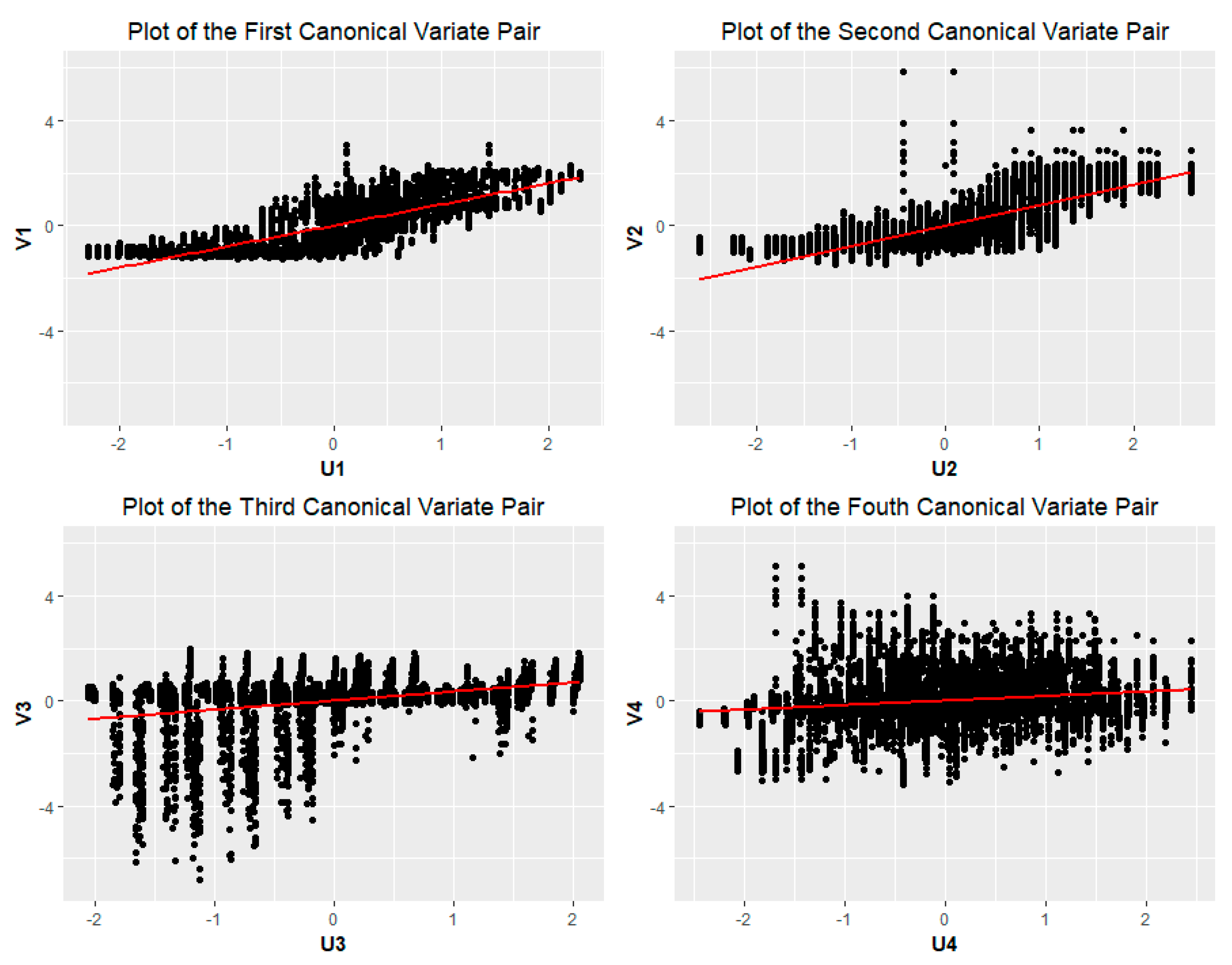
Note that we also tested if there was a relationship between the response variables $Y_i$(where $Y_i$ for $i=1,\dots ,4$ stands for CCD, ICD, CWD, and IWD, i.e., the number of CCDs, ICDs, CWDs, and IWDs made during each simulation run) and the predictor variables $X_i$(where $X_i$for $i=1,\dots ,4$ stands for the factors CCP, fear, desire, and KBT) using the F-test. In this case, we defined that $\mathit{Y}=\mathit{X}\mathit{\beta }+\mathit{\epsilon }$, where $\mathit{Y}=\left(Y_1,\dots ,Y_4\right),$ $\mathit{X}=\left(X_1,\dots ,X_4\right)$, $\mathit{\beta }$ is the coefficient vector for the predictor variable X, and $\mathit{\epsilon }$ is the residual vector. The null hypothesis was $\mathit{\beta }=0$. Because of the small p-value in CV 1, we had enough evidence to claim that response variables and predictor variables were significantly correlated, which means that the model factors had substantial effects on the decision-making abilities of agents. Furthermore, by looking at the squared canonical correlation values in Table 2, we noticed that 64.02% of the variation in $V_1$ was explained by the variation in $U_1$, and 61.39% of the variation in $V_2$ was explained by the variation in $U_2$, but only little variation was explained by the third and the fourth canonical correlation pairs. These findings imply that the first and the second canonical variate pairs captured the most explained variation; therefore, we could focus on these two components in the further analysis. Figure 2 displays the plots of the canonical variate pairs of agents’ decisions against the canonical variates of configuration parameters for each canonical variate pair. The regression line reveals the level of performance of the canonical variates. From the results displayed on Figure 2, we can see that the fitting of the regression line performed better in the first row than in the second row. Thus, this demonstrates that only the first two canonical variate pairs were important and should be considered.

4.2. Estimated Coefficients and Canonical Loadings

The canonical coefficients of the linear combination of $\mathit{X}=\left(X_1,\dots ,X_4\right)$ and $\mathit{Y}=\left(Y_1,\dots ,Y_4\right)$ variables, i.e., of the predictor variables CCP, fear, desire, and KBT and the response variables CCD, ICD, CWD, and IWD, are listed in

Table 3. The canonical coefficients for CCP, fear, desire, and KBT in terms of $U_1$ , $U_2$.

Canonical Coefficients for the Predictor Variables
Canonical Variable	CCP	Fear	Desire	KBT
$U_1$	−1.494665	1.708113	−0.368795	−1.325802
$U_2$	−1.806909	−1.450916	1.7989053	−0.5329955

and

Table 4. The canonical coefficients for CCD, ICD, CWD, and IWD in terms of $V_1$ , $V_2$.

Canonical Coefficients for the Response Variables
Canonical Variable	CCD	ICD	CWD	IWD
$V_1$	−0.004826	0.024058	−0.000220	−0.000168
$V_2$	0.000557	0.106088	−0.001197	0.000023

, respectively. Note that only the first two canonical variates were considered.

Based on the values of the canonical coefficients shown in Table 3 and Table 4, we concluded the following:

(1)

CCP, desire, and KBT had negative contributions in the first canonical variate U₁, while fear had a positive effect.

(2)

For the second canonical variate U₂, CCP, fear, and KBT played negative roles, while desire played a positive role.

(3)

Since the magnitudes of the coefficients represent the contributions of the individual factors to the corresponding canonical variable, it seems that the fear effect was significant in ${\mathrm{U}}_1$, and the CCP and desire effects were significant in ${\mathrm{U}}_2$. As described in Section 3.1, the first canonical pair accounted for the largest correlation; thus, fear seems to be the most influential parameter.

(4)

The magnitudes of the coefficients were also related to the variances of the variable sets. Unlike the small variance in predictor variables, the variances of responses were much larger, and we could not determine the contributions of the responses directly. Thus, we focused on the canonical loadings.

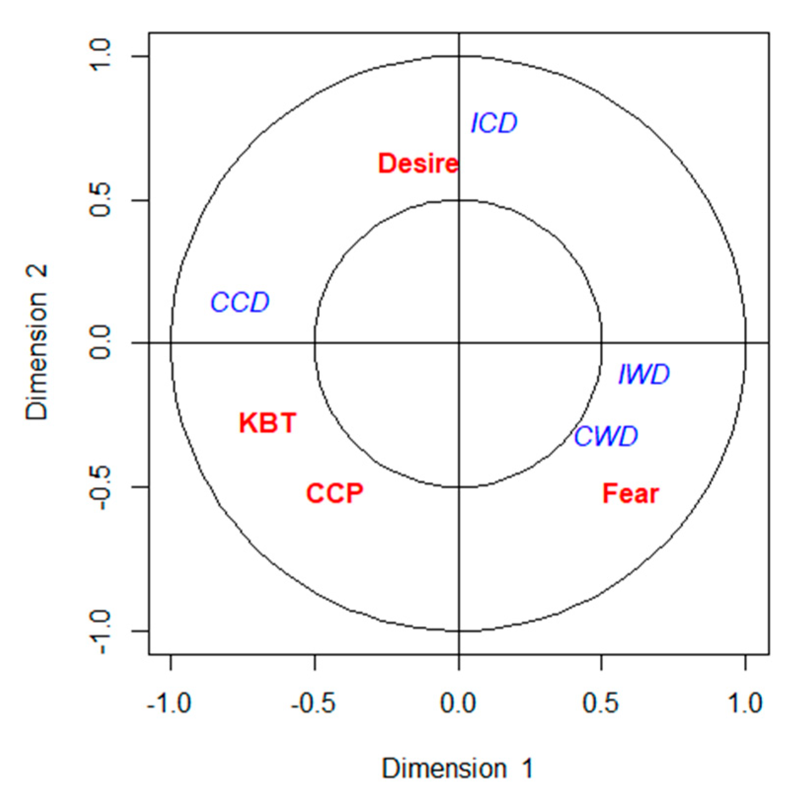
The canonical loadings are defined as the correlations between the explanatory variables and the canonical variates [44]. The plot of canonical loadings for each parameter and each type of decision is displayed in Figure 3. Dimension 1 refers to CV 1 and Dimension 2 refers to CV 2. If a variable is within the inner circle, it suggests that this variable is not strongly correlated with the canonical variates. In other words, this variable is not an essential factor or an important response variable in our model. However, in our case, all the variables were between the inner circle and the outer circle, which means that they all had significant influence that could not be omitted in our model structure. In addition, the distribution of the four types of decisions is dispersed in Figure 3, which suggests that they were significantly different from each other, and that we should analyze them separately.

Based on the canonical correlation analysis, we conclude that there was a strong relationship between the model factors and the decision types, and all factors played important roles in the simulated model. More importantly, desire was negatively associated with ICD through the first canonical variate, but it was significantly positively associated with ICD through the second canonical variate. This may suggest that, with the increase in desire level, ICD firstly decreases and then increases. However, desire and CCD were positively associated through both canonical variates; this may indicate that desire is the driving force for the same direction of change of CCD. Next, we were interested in how the parameters, particularly KBT and CCP, affected each type of decision.

4.3. Regression Tree Results of Autonomous Agents’ Decisions

By using regression trees, we could explore how the model’s factors affected each type of decision and determine which factors played a dominant role in each decision type.

4.3.1. Analysis of CCDs

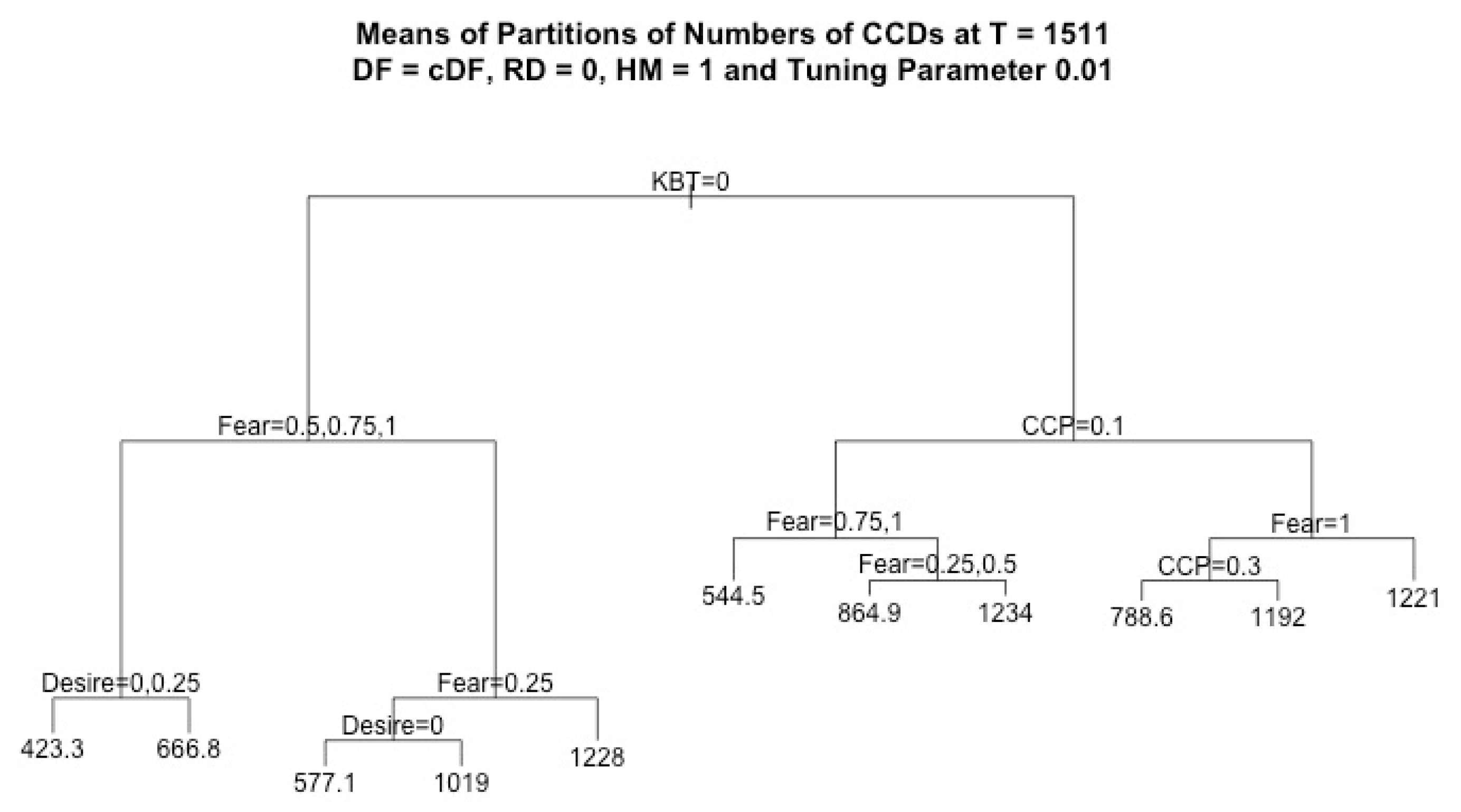
In Figure 4, the plot of the regression tree shows that the most important factor associated with the numbers of CCDs was the KB transfer. When KB transfer did not take place, the predicted mean numbers of CCDs were between 423.3 and 1,228, depending on fear and desire values. The next crucial factor influencing the numbers of CCDs was fear. Conditional on KBT = 0, when fear = 0, the mean number of CCDs was 1,228, which was the largest value compared with the values corresponding to fear being 0.25, 0.5, 0.75, or 1. Thus, in the case of KBT = 0, the agents with no fear were more likely to cross the highway successfully. The third split in the left panel of the regression tree is based on desire parameter values. Conditional on KBT = 0, and fear = 0.5, 0.75, or 1, the mean value of CCDs was 423.3 for desire values 0 or 0.25, while the mean value was 666.8 for desire values 0.5, 0.75, or 1. If KBT = 0, and fear = 0.25, the predicted mean value became 577.1 when desire = 0; otherwise, the mean number of CCDs was 1,019. Thus, when KBT = 0, and fear was greater than 0, the higher values of desire had a positive effect on the mean numbers of CCDs. Focusing on the right part of the tree, CCP = 0.1 was the second condition to split the tree.

However, in both cases of CCP = 0.1 and CCP > 0.1, we can infer that the mean value of the number of CCDs had a lower value when agents experienced a stronger intensity of fear.

Based on the analysis above, we concluded the following:

• KBT played a dominant role in partitioning the numbers of CCDs.
• When KBT is 0, fear was the second important factor; however, when KBT is 1, the traffic density, which was determined by CCP, controlled the tree branching.
• For both values of KBT, the decrease in the value of fear increased the average number of CCDs.
• If KBT = 0 and the agents experienced fear, then the agents which had more desire to cross the highway had higher success in crossing.

4.3.2. Analysis of ICDs

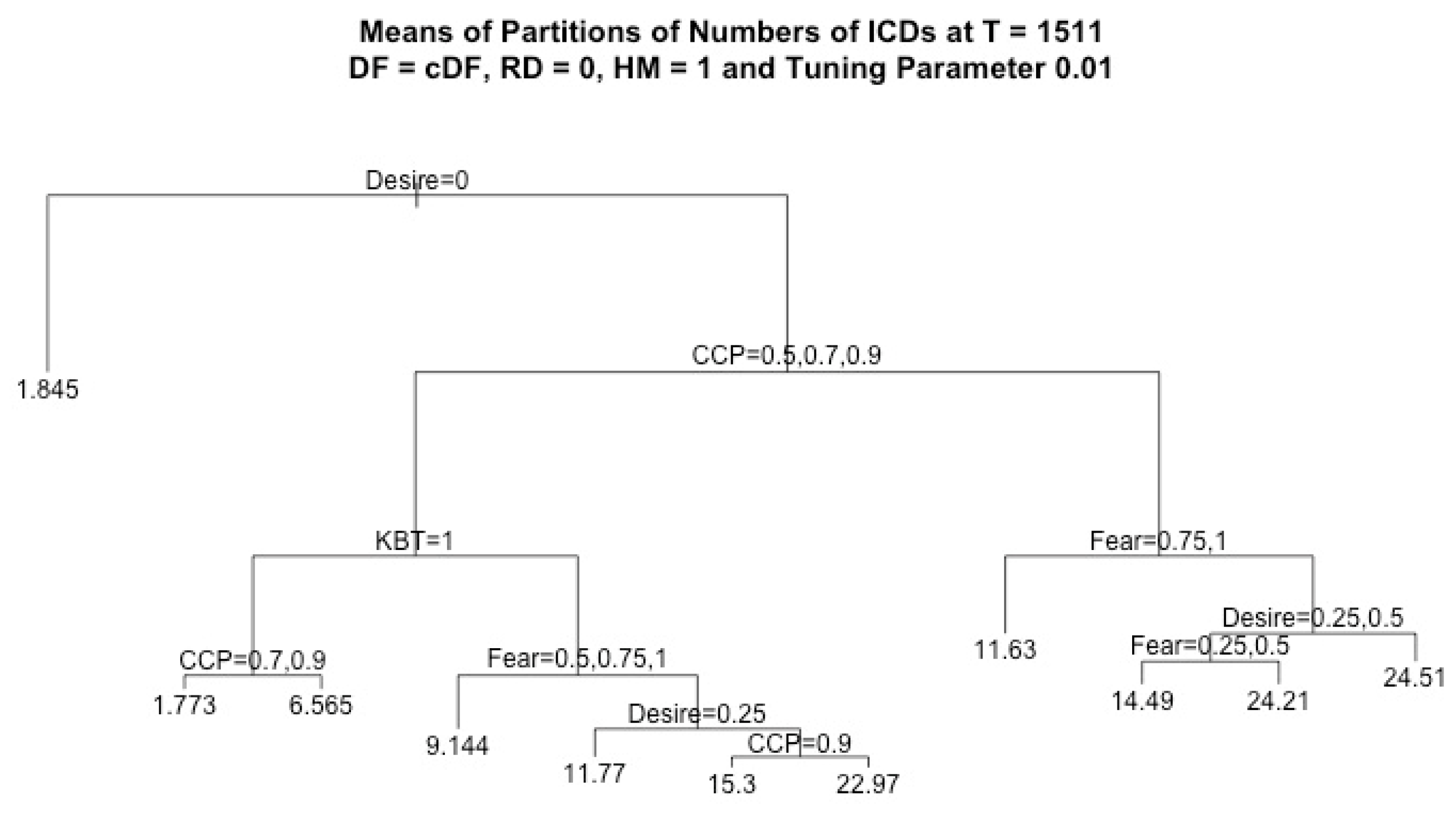
In Figure 5, the regression tree modeling result of the numbers of ICDs shows the following:

• Desire was the main factor affecting the numbers of ICDs. If the agents had no desire, the tree stopped splitting. In other words, regardless of the changes in the values of the other factors, if desire = 0, then the predicted value of mean numbers of ICDs was 1.845.
• When desire was greater than 0, then the next factor affecting the numbers of ICDs was CCP. If CCP was 0.1 or 0.3, then the KB transfer did not influence the numbers of ICDs, because KB transfer only took place once from the agents in an environment with CCP = 0.1 to the agents in an environment with CCP = 0.3. However, when CCP exceeded 0.3, i.e., when KB transfer took place several times, then the KBT reduced the numbers of ICDs. Thus, this demonstrates that, with more information/knowledge accumulation, even the agents with desire made a lower number of ICDs.
• When desire was not 0, and the traffic density was the highest (i.e., CCP = 0.9), then the agents with higher fear values had the smaller numbers of ICDs.

4.3.3. Analysis of CWDs

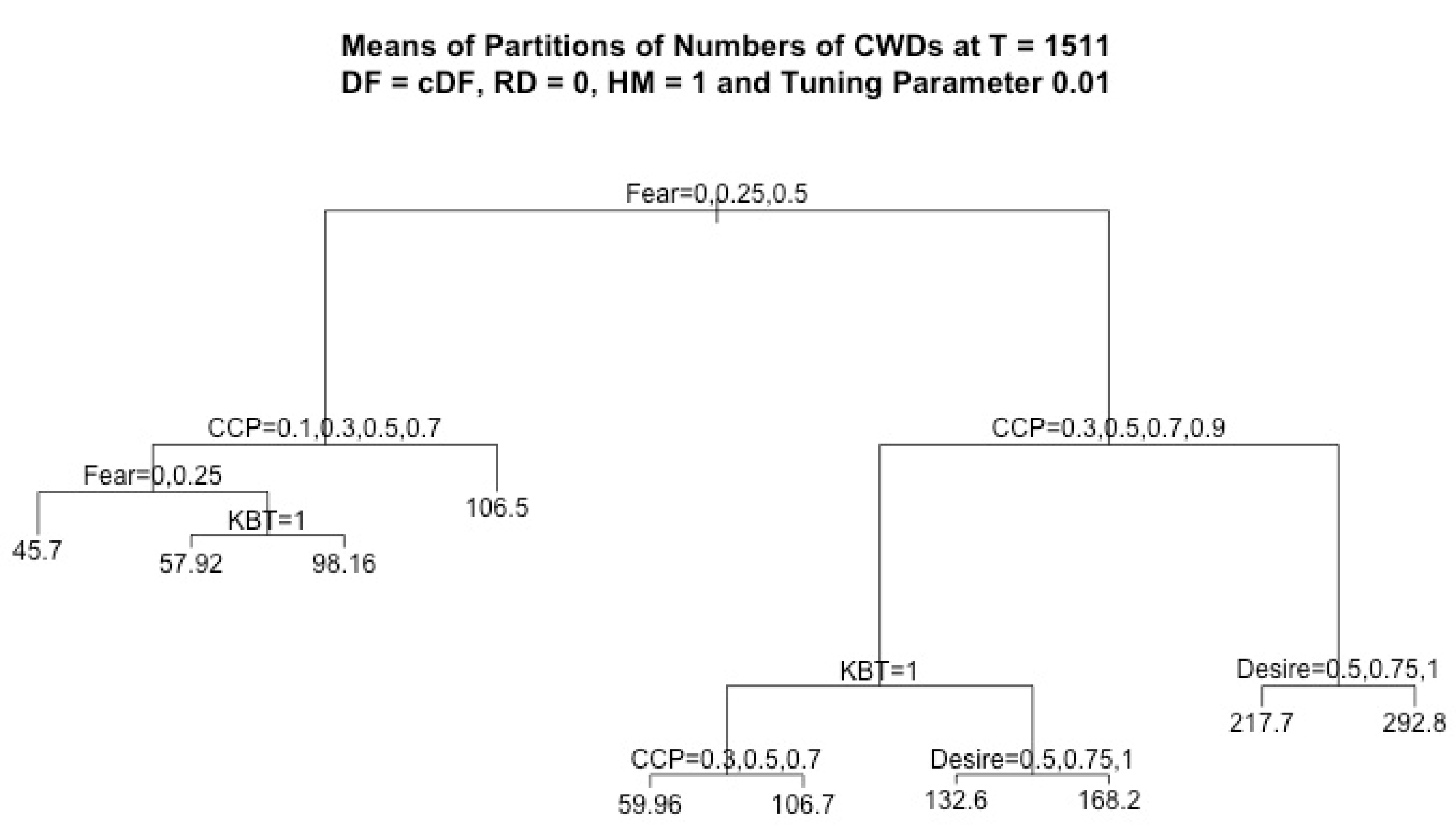
According to the tree for the numbers of CWDs shown in Figure 6, we concluded the following:

• The decisive factor influencing the numbers of CWDs was fear, and then CCP.
• Conditional on fear = 0, 0.25, or 0.5, when CCP = 0.9, the predicted mean number of CWDs was 106.5, which was the highest value compared to any other lower traffic density (i.e., lower value of CCP). In contrast, conditional on fear = 0.75 or 1, when CCP = 0.1, the predicted mean of numbers of CWDs belonged to the interval [217.7, 292.8]. These numbers were much larger than the ones for the values of CCP higher than 0.1.
• When fear was 0, 0.25, or 0.5, KB transfer did not affect the mean values of CWDs significantly. However, when fear was 0.75 or 1, KBT = 1, and CCP was greater than 0.1, the repeated transferring of KB increased the numbers of CWDs, and, when CCP = 0.9, the mean number of CWDs was 106.70, whereas, when CCP = 0.3, 0.5, or 0.7, it was only 59.96.

4.3.4. Analysis of IWDs

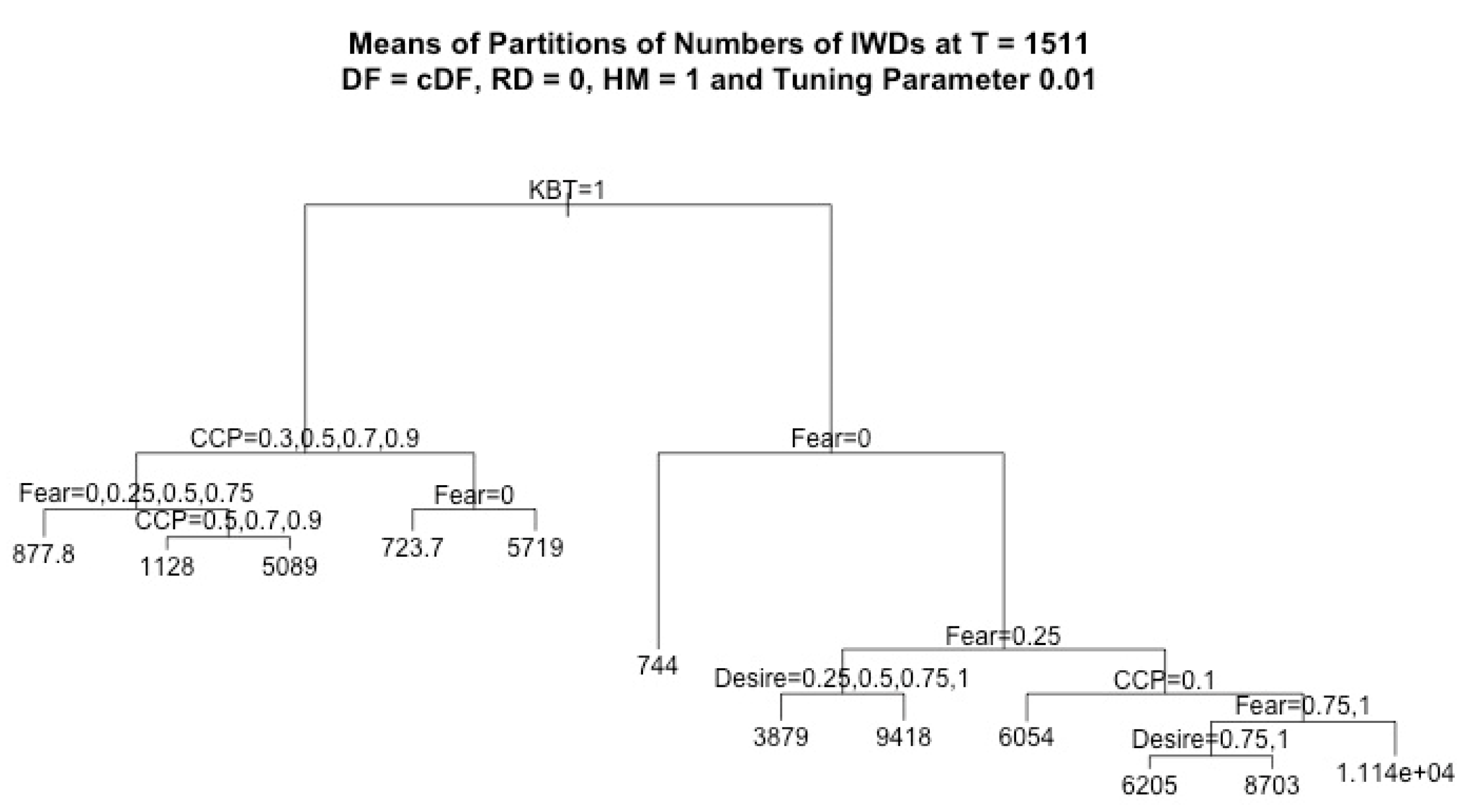
Based on the results shown in Figure 7, the predictions of the mean numbers of IWDs can be summarized as follows:

• KBT was the dominant factor splitting the data in terms of the mean values of IWDs. If the transfer of KB took places, then the predictive mean values of IWDs were between 877.8 and 5719, whereas, if there was no KB transfer, then the mean values of numbers of IWD were within [744, 11,140]. This confirms that KB transfer could lower the numbers of IWDs.
• When KBT = 1, CCP was the second influential factor, followed by fear, whereas, when KBT = 0, the mean values of the numbers of IWDs depended on the factor fear, and next on desire and CCP.
• Conditional on KBT = 0, the estimated mean values of IWDs were 744 when fear = 0, between 3879 and 9418 when fear = 0.25, 11,140 when fear = 0.5, and between 6205 and 8703 when fear = 0.75 or 1. Thus, when KBT = 0, the estimated mean values of the numbers of IWDs reached the peak when fear = 0.5, and agents without fear made the smallest numbers of wrong waiting decisions.

Based on the results displayed in Figure 4, Figure 5, Figure 6, Figure 7, we can conclude that the regression tree results for the mean numbers of CCDs and IWDs had similar characteristics, and the KB transfer was the most important factor influencing the numbers of these decisions, followed by the factors CCP and fear. On the other hand, when considering the numbers of ICDs and CWDs, the KB transfer became the third most important factor. However, when the KB transfer was applied, the values of mean numbers of ICDs decreased, and the numbers of CWDs went up. Also, the higher values of fear promoted higher numbers of both CWDs and IWDs, but lower numbers of CCDs.

5. Conclusions and Remarks

For a better understanding of the nature of complex systems modeling, computer simulations and the analysis of the resulting data are major tools which can be successfully applied. In this work, we studied how cognitive agents’ decisions in learning to cross a CA-based highway depend on the values of the model's factors. Within the study, canonical correlation analysis of the simulation data was firstly used to identify the significant correlations between the model’s response variables and the independent variables. It justified that all the model’s parameters and decision types were strongly correlated, and no variables, i.e., model parameters and decision types, could be omitted in the analysis of the data of the simulated model. Regression tree analysis was then conducted to identify which model’s factors affected the mean values of agents’ decisions the most. The results obtained from the regression tree analysis demonstrated that, when agents were allowed to change their initial crossing point, for correct crossing decisions (CCDs) and incorrect waiting decisions (IWDs), the KB transfer was the most important factor influencing the numbers of these decisions, and CCP and fear were the second most influential parameters, whereas, for incorrect crossing decisions (ICDs) and correct waiting decisions (CWDs), fear and desire were the most crucial parameters, and KB transfer was the third most important factor. Thus, the accumulation of agents’ knowledge about their performance in learning to cross the highway, even in some other traffic environment, improved the agents’ decision-making abilities. Also, the presented statistical methodologies can be useful in modeling and analyzing data of similar computer simulation models when the aim is a better understanding of the factor or treatment effects.

In this paper, we only discussed the agents’ learning performance when they used the crossing-based decision formula (cDF). The comparisons of the agents’ learning performance when they use cDF with their performance when they use cwDF (i.e., the crossing-and-waiting-based decision formula) instead will be discussed elsewhere. This will provide insight into the effects of the feedback mechanisms on the agents’ learning performance. The decision formula cDF provides only the feedback about the correctness of the agents’ crossing decisions, while the decision formula cwDF provides feedback to the agents about the correctness of both their crossing and waiting decisions. Thus, it will be interesting and important to investigate if and how much the additional feedback information may improve the agents’ learning performance. Providing feedback to the agents about the correctness of both their crossing and waiting decisions will be more computationally intensive than providing the feedback only about the correctness of their crossing decisions. The reason is that the implementation of the decision formula cwDF requires following the movement of the incoming car longer and additional assessments compared to the decision formula cDF. The understanding of the potential benefits and costs of using the decision algorithm cwDF instead of cDF will be important in potential hardware implementation in robotics.

In our model, we simulated the traffic environment in which a cognitive agent, being an abstraction of an autonomous vehicle, tried to learn how to successfully cross a country highway. This model of a very simplified intersection provided insight into the effects of various factors and their interactions on the agents’ learning performance. In the future, we plan to extend the model to simulate more complexed and realistic types of road intersections, and we plan to investigate the cognitive agents’ learning performance in crossing such intersections. Also, in the presented model, an incoming car never reacts, i.e., changes its behavior, upon seeing an agent attempting to cross the country highway. In the future, we plan to extend the model and investigate the effects of an incoming car and cognitive agent interactions, i.e., changing behaviors, on the agents’ learning performance in crossing an intersection.

References

- Li, B.H.; Hou, B.C.; Yu, W.T.; Lu, X.B.; Yang, C.W. Applications of artificial intelligence in intelligent manufacturing: A review. Front. Inf. Technol. Electron. Eng. 2017, 18, 86–96. [Google Scholar] [CrossRef]
- Pham, D.T.; Pham, P.T.N. Artificial intelligence in engineering. Int. J. Mach. Tools Manuf. 1999, 39, 937–949. [Google Scholar] [CrossRef]
- Jourdan, Z.; Rainer, R.K.; Marshall, T.E. Business intelligence: An analysis of the literature. Inf. Syst. Manag. 2008, 25, 121–131. [Google Scholar] [CrossRef]
- Chairman-Mertens, K. Artificial intelligence and pattern recognition. In Proceedings of the 1985 ACM Thirteenth Annual Conference on Computer Science, New Orleans, LA, USA; ACM: New York, NY, USA, 1985; p. 420. [Google Scholar]
- Bishop, C.M. Pattern Recognition and Machine Learning; Springer: Berlin/Heidelberg, Germany, 2006. [Google Scholar]
- Davis, J.C.; Vasanth, K.; Saxena, S.; Mozumder, P.K.; Rao, S.; Fernando, C.L.; Burch, R.G. Method and system for using response-surface methodologies to determine optimal tuning parameters for complex simulators. U.S. Patent No. 6,381,564, 30 April 2002. [Google Scholar]
- Pires, T.S.; Cruz, M.E.; Colaço, M.J. Response surface method applied to the thermoeconomic optimization of a complex cogeneration system modeled in a process simulator. Energy 2013, 52, 44–54. [Google Scholar] [CrossRef]
- Mendenhall, W.; Sincich, T.; Boudreau, N.S. A Second Course in Statistics: Regression Analysis; Prentice Hall: Upper Saddle River, NJ, USA, 1996; Volume 5. [Google Scholar]
- Mitchell, M. Complex systems: Network thinking. Artif. Intell. 2006, 170, 1194–1212. [Google Scholar] [CrossRef] [Green Version]
- Weisbuch, G. Complex Systems Dynamics; CRC Press: Boca Raton, FL, USA, 2018. [Google Scholar]
- Ray, A. Symbolic dynamic analysis of complex systems for anomaly detection. Signal Process. 2004, 84, 1115–1130. [Google Scholar] [CrossRef]
- Lotz, A.; Inglés-Romero, J.F.; Stampfer, D.; Lutz, M.; Vicente-Chicote, C.; Schlegel, C. Towards a stepwise variability management process for complex systems: A robotics perspective. In Artificial Intelligence: Concepts, Methodologies, Tools, and Applications; IGI Global: Hershey, PA, USA, 2017; pp. 2411–2430. [Google Scholar]
- Giusti, A.; Guzzi, J.; Cireşan, D.C.; He, F.L.; Rodríguez, J.P.; Fontana, F.; Scaramuzza, D. A machine learning approach to visual perception of forest trails for mobile robots. IEEE Robot. Autom. Lett. 2015, 1, 661–667. [Google Scholar] [CrossRef]
- Stone, P.; Veloso, M. Multiagent systems: A survey from a machine learning perspective. Auton. Robot. 2000, 8, 345–383. [Google Scholar] [CrossRef]
- Navarro, I.; Matía, F. An introduction to swarm robotic. ISRN Robot. 2012, 2013. [Google Scholar] [CrossRef]
- Di Stefano, B.N.; Lawniczak, A.T. Modeling a simple adaptive cognitive agent. Acta Phys. Pol. B Proc. Suppl. 2012, 5, 21–29. [Google Scholar] [CrossRef]
- Lawniczak, A.T.; Ernst, J.B.; Di Stefano, B.N. Creature learning to cross a ca simulated road. In Proceedings of the International Conference on Cellular Automata, Santorini, Greece, 24–27 September 2012; Springer: Berlin/Heidelberg, Germany, 2012; pp. 425–433. [Google Scholar]
- Lawniczak, A.T.; Ernst, J.B.; Di Stefano, B.N. Simulated naïve creature crossing a highway. Procedia Comput. Sci. 2013, 18, 2611–2614. [Google Scholar] [CrossRef]
- Lawniczak, A.T.; Di Stefano, B.N.; Ernst, J.B. Software implementation of population of cognitive agents learning to cross a highway. In Proceedings of the International Conference on Cellular Automata, Kraków, Poland, 22–25 September 2014; Springer: Cham, Switzerland, 2014; pp. 688–697. [Google Scholar]
- Lawniczak, A.T.; Yu, F. Comparison of Agents’ Performance in Learning to Cross a Highway for Two Decisions Formulas. In Proceedings of the 9th International Conference on Agents and Artificial Intelligence, Porto, Portugal, 24–26 February 2017; pp. 208–219. [Google Scholar]
- Lawniczak, A.T.; Yu, F. Decisions and Success of Heterogeneous Population of Agents in Learning to Cross a Highway. In Proceedings of the 2017 IEEE Symposium Series on Computational Intelligence. IEEE SSCI 2017, Honolulu, HI, USA, 27 November–1 December 2017. [Google Scholar]
- Lawniczak, A.T.; Yu, F. Cognitive Agents Success in Learning to Cross a CA Based Highway Comparison for Two Decision Formulas. Procedia Comput. Sci. 2017, 108, 2443–2447. [Google Scholar] [CrossRef]
- Schumacker, R.E. Using R with Multivariate Statistics; Sage Publications: Thousand Oaks, CA, USA, 2015. [Google Scholar]
- Mazuruse, P. Canonical correlation analysis: Macroeconomic variables versus stock returns. J. Financ. Econ. Policy 2014, 6, 179–196. [Google Scholar] [CrossRef]
- Fox, S.; Hammond, S. Investigating the multivariate relationship between impulsivity and psychopathy using canonical correlation analysis. Personal. Individ. Differ. 2017, 111, 187–192. [Google Scholar] [CrossRef]
- Yang, J.; Sun, W.; Liu, N.; Chen, Y.; Wang, Y.; Han, S. A Novel Multimodal Biometrics Recognition Model Based on Stacked ELM and CCA Methods. Symmetry 2018, 10, 96. [Google Scholar] [CrossRef]
- Delisle-Rodriguez, D.; Villa-Parra, A.C.; Bastos-Filho, T.; López-Delis, A.; Frizera-Neto, A.; Krishnan, S.; Rocon, E. Adaptive Spatial Filter Based on Similarity Indices to Preserve the Neural Information on EEG Signals during On-Line Processing. Sensors 2017, 17, 2725. [Google Scholar] [CrossRef]
- Breiman, L.; Friedman, J.; Olshen, R.A.; Stone, C.J. Olshen, Classification and Regression Trees; Taylor & Francis: Abingdon, UK, 1984. [Google Scholar]
- Lemon, S.C.; Roy, J.; Clark, M.A.; Friedmann, P.D.; Rakowski, W. Classification and regression tree analysis in public health: Methodological review and comparison with logistic regression. Ann. Behav. Med. 2003, 26, 172–181. [Google Scholar] [CrossRef] [PubMed]
- Yamashita, T.; Noe, D.A.; Bailer, A.J. Risk Factors of Falls in Community-Dwelling Older Adults: Logistic Regression Tree Analysis. Gerontologist 2012, 52, 822–832. [Google Scholar] [CrossRef] [Green Version]
- Skedgell, K.; Kearney, C.A. Predictors of school absenteeism severity at multiple levels: A classification and regression tree analysis. Child. Youth Serv. Rev. 2018, 86, 236–245. [Google Scholar] [CrossRef]
- Reis, J.P.; Pereira, A.; Reis, L.P. Coastal ecosystems simulation: A decision tree analysis for Bivalve’s growth conditions. In Proceedings of the 26th European Conference on Modelling and Simulation, Koblenz, Germany, 29 May–1 June 2012. [Google Scholar]
- Molina-Delgado, M.; Padilla-Mora, M.; Fonaguera, J. Simulation of behavioral profiles in the plus-maze: A Classification and Regression Tree approach. Biosystems 2013, 114, 69–77. [Google Scholar] [CrossRef]
- Lin, X.S. Introductory Stochastic Analysis for Finance and Insurance; John Wiley & Sons: Hoboken, NJ, USA, 2006; Volume 557. [Google Scholar]
- Lawniczak, A.T.; Ly, L.; Yu, F.; Xie, S. Effects of Model Parameter Interactions on Naïve Creatures’ Success of Learning to Cross a Highway. In Proceedings of the 2016 IEEE Congress on Evolutionary Computation, IEEE CEC 2016, Part of IEEE World Congress on Computational Intelligence (IEEE WCCI), Vancouver, BC, Canada, 24–29 July 2016; pp. 693–702. [Google Scholar]
- Lawniczak, A.T.; Ly, L.; Xie, S.; Yu, F. Effects of Agents’ Fear, Desire and Knowledge on Their Success When Crossing a CA Based Highway. In Cellular Automata. LNCS (9863); El Yacoubi, S., Wąs, J., Bandini, S., Eds.; Springer: Cham, Switzerland, 2016; pp. 446–455. [Google Scholar]
- Lawniczak, A.T.; Ly, L.; Yu, F. Effects of Simulation Parameters on Naïve Creatures Learning to Safely Cross a Highway on Bimodal Threshold Nature of Success. Procedia Comput. Sci. 2016, 80, 2382–2386. [Google Scholar] [CrossRef]
- Lawniczak, A.T.; Di Stefano, B.N.; Ly, L.; Xie, S. Performance of Population of Naïve Creatures with Fear and Desire Capable of Observational Social Learning. Acta Phys. Pol. B Proc. Suppl. 2016, 9, 95–107. [Google Scholar] [CrossRef]
- Ly, L.; Lawniczak, A.T.; Yu, F. Exploration of Simulated Creatures Learning to Cross a Highway Using Frequency Histograms. Procedia Comput. Sci. 2016, 95, 418–427. [Google Scholar] [CrossRef] [Green Version]
- Ly, L.; Lawniczak, A.T.; Yu, F. Quantifying Simulation Parameters’ Effects on Naïve Creatures Learning to Safely Cross a Highway using Regression Trees. Acta Phys. Pol. B Proc. Suppl. 2016, 9, 77–93. [Google Scholar] [CrossRef]
- Lawniczak, A.T.; Ly, L.; Yu, F. Success Rate of Creatures Crossing a Highway as a Function of Model Parameters. Procedia Comput. Sci. 2016, 80, 542–553. [Google Scholar] [CrossRef] [Green Version]
- Nagel, K.; Schreckenberg, M. A cellular automaton model for freeway traffic. J. Phys. I 1992, 2, 2221–2229. [Google Scholar] [CrossRef]
- Alonso, E.; d’Inverno, M.; Kudenko, D.; Luck, M.; Noble, J. Learning in multi-agent systems. Knowl. Eng. Rev. 2001, 16, 277–284. [Google Scholar] [CrossRef] [Green Version]
- Härdle, W.; Simar, L. Applied Multivariate Statistical Analysis; Springer: Berlin, Germany, 2007; Volume 22007, pp. 1051–8215. [Google Scholar]
Figure 1.
The diagram describes three main components of the simulation model: highway, vehicles, and agents. In our simulation, agents are generated at the crossing point (CP) = 60 and they can move randomly to the neighboring crossing points. Each simulation run features 1511 time steps.
Figure 2.
The scatter plots for each canonical variate pair with the fitted regression line.
Figure 3.
The canonical loadings for correct and incorrect crossing decisions (CCD, ICD), correct and incorrect waiting decisions (CWD, IWD), car creation probability (CCP), fear, desire, and knowledge base transfer (KBT) in Dimension 1 (Canonical Variate 1) and Dimension 2 (Canonical Variate 2).
Figure 4.
Tree model for means of partition numbers of CCDs at simulation end, with parameters RD = 0, HM = 1, and tuning parameter = 0.01, when agents used cDF. For each node, the left branch is conditional on the node being true.
Figure 5.
Tree model for means of partition numbers of ICDs at simulation end with parameters RD = 0, HM = 1, and tuning parameter = 0.01, when agents used cDF. For each node, the left branch is conditional on the node being true.
Figure 6.
Tree model for means of partition numbers of CWDs at the simulation end with parameters RD = 0, HM = 1, and tuning parameter = 0.01, when agents used cDF. For each node, the left branch is conditional on the node being true.
Figure 7.
Tree model for means of partition numbers of IWDs at the simulation end with parameters RD = 0, HM = 1, and tuning parameter = 0.01, when agents use cDF. For each node, the left branch is conditional on the node being true.