Investigation of the Horizontal Motion of Particle-Laden Jets


1
Department of Civil and Building Engineering, University of Sherbrooke, Sherbrooke, QC J1K 2R1, Canada
2
Department of Mechanical Engineering, Amirkabir University of Technology, Tehran 1591634311, Iran
3
Department of Mechanical Engineering, Lakehead University, Thunder Bay, ON P7B 5E1, Canada
*
Author to whom correspondence should be addressed.
Computation 2020, 8(2), 23; https://0-doi-org.brum.beds.ac.uk/10.3390/computation8020023
Submission received: 15 January 2020
/
Revised: 1 April 2020
/
Accepted: 2 April 2020
/
Published: 8 April 2020
(This article belongs to the Special Issue Computational Heat, Mass, and Momentum Transfer—II)
Abstract
:Particle-laden jet flows can be observed in many industrial applications. In this investigation, the horizontal motion of particle laden jets is simulated using the Eulerian–Lagrangian framework. The two-way coupling is applied to the model to simulate the interaction between discrete and continuum phase. In order to track the continuum phase, a passive scalar equation is added to the solver. Eddy Life Time (ELT) is employed as a dispersion model. The influences of different non-dimensional parameters, such as Stokes number, Jet Reynolds number and mass loading ratio on the flow characteristics, are studied. The results of the simulations are verified with the available experimental data. It is revealed that more gravitational force is exerted on the jet as a result of the increase in mass loading, which deflects it more. Moreover, with an increase in the Reynolds number, the speed of the jet rises, and consequently, the gravitational force becomes less capable of deviating the jet. In addition, it is observed that by increasing the Stokes number, the particles leave the jet at higher speed, which causes a lower deviation of the jet.
1. Introduction
Particle-laden jet flows have various engineering applications, such as fuel injection in internal combustion engines. In this regard, the jets laden with particles have been investigated by many researchers experimentally and computationally [1,2,3,4,5,6,7,8,9,10,11,12,13,14,15]. Many approaches have been used to experimentally analyze the jets laden with particles like Phase-Doppler Anemometry (PDA), Laser-Doppler Anemometry (LDA) and high-speed camera image processing. Fundamental experiments on dilute particle jets by the use of LDA can be found in [1,2,3,4]. Fan et al. investigated the effect of dispersed phase on the flow characteristics of a coaxial jet with particles laden. They showed when the particle ratio increases, the spreading ratio decreases [2]. Puttinger et al. analyzed the dilute particle-laden flow by using high-speed camera and image processing [5]. Due to the high spatial and temporal resolution of the latter method, it can be employed to study the turbulent flow with a high concentration ratio. This can be used for a wide variety of data and does not depend on the preset parameters. Generally, there are two main methods to simulate particle-laden flow, namely Eulerian–Eulerian and Eulerian–Lagrangian [6]. The former is used when the continuum assumption can be applied for both phases, while the latter is applied when particles constitute dispersed phases and fluid constitutes continuum phases. Both techniques have pros and cons [6]. A major problem of the first method is that some information such as the motion of the individual particles, and the collision between particles are not considered. In addition, applying boundary conditions for the second phase is challenging. However, the advantage of the Eulerian–Eulerian method is that the same equation and numerical methods are applied to both phases. In the Eulerian–Lagrangian method, more detailed information about the motion of particles and their interaction with the surrounding can be obtained. However, some computational difficulties arise when the number of particles increases or the size of particles decreases. For instance, when the size of particles decreases, the effect of turbulent eddies on particles should be calculated even in smaller sizes; therefore, the cost of the computational method will be increased. Wang et al. [7] simulated the particle-laden jet using the Eulerian–Lagrangian method. In their study, the gas-phase and fluid-phase velocities show good agreement with the experimental results. They investigated the effects of different parameters on the flow behavior, including particle size, Stokes number and mass loading ratio. The Stokes number () is defined as the ratio of the characteristic time of a Lagrangian phase () to a characteristic time of the continuum phase (). The Eulerian–Eulerian method was applied to simulate particle-laden jet turbulent flow in Ref [8]. In their research, the major roles of the particle size and loading ratio on the flow characteristic of particle-laden jets are shown. The Eulerian–Lagrangian method was employed by Jebakumar and Abraham [9] in which the changes in centerline velocities and spreading rate were investigated by varying parameters such as fluctuating particle velocity at the jet inlet, gas-phase turbulence intensity. Lue et al. showed the major effect of Stokes numbers on the clustering of particles by means of one-way coupling direct numerical simulation of a turbulent particle-laden jet [10]. The effect of the Stokes number on the particle motion and turbulent characteristics of particle-laden flow in the channel was investigated by Lee [11]. They found, for Stokes number of 5 that the particles increase the flow turbulence, while increasing the Stokes number of particles leads to decreasing the turbulence. The coupling behavior of solid particles and fluid makes modeling of this process complex. The coupling between solid and fluid phases has a substantial impact on multi-phase flows. If fluid exerts effects on particle motion but no reverse influence exists, the flow is called one-way coupling regime. If both phases have impacts on each other, the flow is called two-way coupling regime. In addition, if the collision between particles becomes important, the flow is called 4-way coupling regime. The Stokes number and concentration or loading ratios are important parameters in particle-laden flows to determine the coupling between solid and fluid phases. For more details, the reader is referred to reference [12]. Numerical simulations were carried out by Wang et al. [7] using one-way coupling in order to estimate the evolution of particles in a plane turbulent wall jet. Kazemi et al. [13] performed a CFD simulation with the assumption of two-way coupling between two phases. They applied three different dispersion models. Their results suggested that the particle loading ratio should be considered in choosing the dispersion model. The Eddy Life Time (ELT) model is considered as one of the conventional dispersion models which can be used to investigate particle dispersion resulted from instantaneous turbulent velocity fluctuations [14]. In the present study, two-way coupling simulation of horizontal turbulent jet laden with particles in Eulerian–Lagrangian framework is conducted employing Reynolds averaged Navier–Stokes (RANS) model and ELT model is employed for modeling particle dispersion. The particle trajectory resulting from the simulation is compared with the experimental results reported by Fleckhaus et al. [15].
The heavy jets, caused by the high difference in density between the jet and surrounding fluid, were investigated by some authors to study the mixing characteristics of wastewater discharge [16,17]. However, there are many industrial applications that contain the discharging process of heavy particles and fluid, which form heavy jets. For example, in industrial wastewater and an exhaust gas flow, which in the effect of solid particles on the jet profile of disposal, wastes must be taken into consideration. In this paper, the effects of three non-dimensional parameters are investigated on the characteristics of heavy jets, which result from heavy particles. The influence of Stokes number, mass loading ratio and Reynolds number (Re = ), where is the Kinematic viscosity of the continuum phase, and mass loading ratio, which is defined mass fraction of the dispersed phase to continuum phase of the jet on the trajectory distribution of jet with particle-laden are investigated. The definition of the Stokes number is based on the Stokes’ relaxation time scale, and this number represents the diameter of the particles with a density of 2590kg/m3. In addition, turbulence modulation is not considered in this work. It shows that the effect of gravity on the motion of the jet can be seen clearly by the trajectory of particles.
2. Governing Equation
In this study, the carrier flow is considered as a continuous phase and particles as dispersed phases, which are simulated using the Eulerian–Lagrangian framework. The two-way coupling is applied to study the interaction between two phases.
2.1. The Eulerian Equations
The gas phase is described by the Reynolds averaged Navier–Stokes equations (RANS) for incompressible flow. The continuity and momentum equations can be written as follows [18]:
with being the density of the gas, the pressure, the velocity in the direction; defines momentum source term because of the interaction between Eulerian and Lagrangian parts; denotes the effective stress tensor which can be defined as below:
where and are kinematic viscosity and turbulent kinematic viscosity, respectively; is the Kronecker delta. Here the turbulent viscosity is computed using the k-ω SST (Shear Stress Transport) turbulence model [19]. In the present study, a passive scalar equation is added to the solver as a tracer to track the gas phase, to investigate different fluid dynamic behavior between the tracer (particles with zero inertia) and inertial particles, which can be described as follows:
In the above equation, Schmidt number and turbulent Schmidt number are 0.4 and 0.7, respectively.
2.2. The Lagrangian Equations
The dispersed phase is composed of parcels. Each parcel is defined by the group of properties including velocity , diameter , density , position , computational weight (ω). The diameter, density and computational weight of parcels are constant after injection. It is assumed that the drag and gravity forces have a dominant effect compared to other forces. Therefore, other forces are neglected. In the case of the heavy particle, i.e., ρ2 >> ρ1, the volume force applied by surrounding fluid flow can be assumed to be equal to the drag force [20].
The drag force acts on a particle which is equal to:
where relative velocity and particle relaxation time can be described as:
Relaxation time is applied to show the resistance of a dispersed phase to adjust to continuum phase motion and is the correction factor, which is defined as below:
is the particle Reynolds number base on the relative velocity which is defined as:
where denotes the instantaneous gas velocity. It is the summation of mean gas flow velocity and fluctuating gas flow velocity. The mean velocity is interpolated at the parcel location from RANS equations; the eddy lifetime dispersion model is applied to calculate the fluctuating velocity. In the ELT model, the fluctuating velocity is defined as [13]:
where is the normally distributed random number of the standardized Gaussian distribution and denotes the turbulent kinetic energy. The updated value fluctuating velocity should be calculated after the characteristic lifetime :
where is a random number between 0 and 1 and Lagrangian integral time scale calculated as:
where is an empirical factor whose value is adjusted based on the experimental results. In many studies, the value for this parameter is chosen as 0.3, which is also applied in the work of Refs [22,23].
The momentum transfer term in Equation (2) calculated for cell in each time step as:
where is the time step, is the volume of the cell, is the Kernel function of the cell, is the statistic weight of the parcel and is the drag force applied on the ith parcel. The momentum transfer term is obtained by the summation of product term for all parcels. The Kernel function is considered as a linear weighted interpolation operator in OpenFoam [24].
3. Analysis and Modeling
To solve the governing equations, open-source OpenFOAM package (www.openfoam.org) is employed. In OpenFOAM, the equations of the continuum phase are solved with the discrete cell-centered finite volume method on the discrete computational grid. The boundary condition at the inlet is a fixed velocity profile, zero gradient at the outlet and no-slip conditions are applied for the walls. The pressure is zero gradient for the inlet, and fixed value (0) applied to the outlet. The Concentration field is of a fixed value for the inlet and zero gradients for all others. The turbulent intensity is 10% for the inlet, and standard wall function k- are used for walls. The parcels are injected at a rate of 1,000,000 per second. Each parcel will be considered omitted after reaching the outlet, and in approaching the wall, they are considered rebounded.
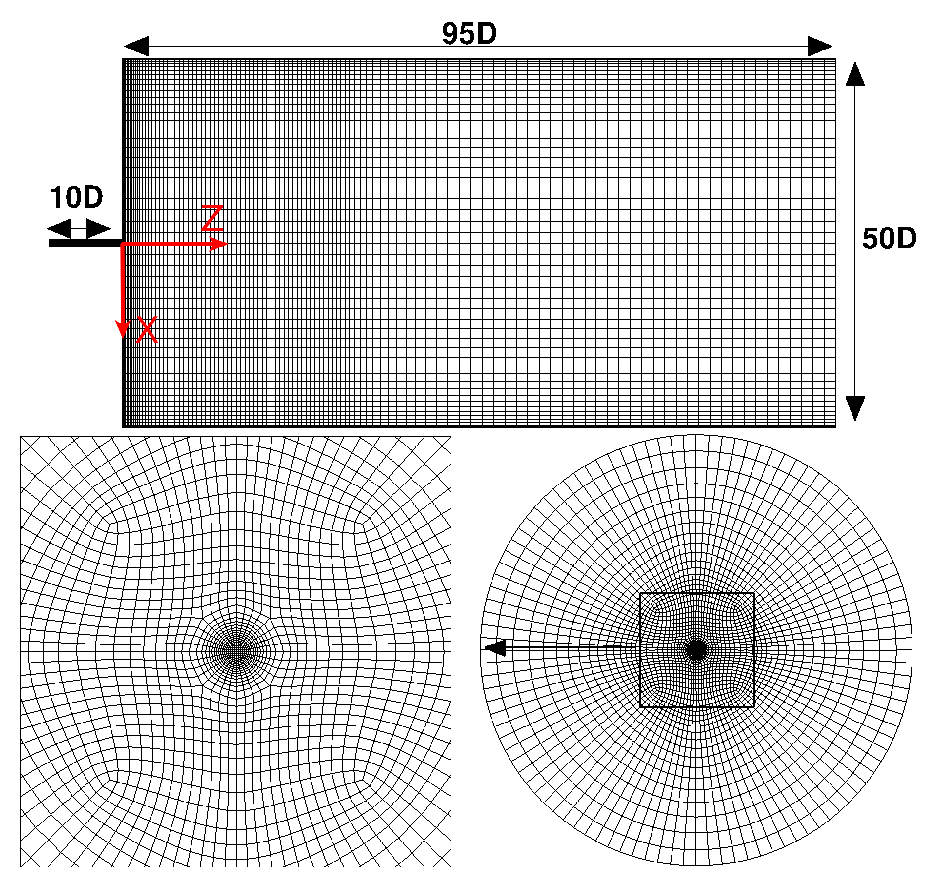
To consider grid independency for our domain, three different grid sizes (1,100,000, 700,000, 400,000) were compared based on the velocity profile of the continuum phase along three sections and . The maximum error was 4% for the 700,000-cell grid. Therefore, the simulations were done using 700,000 cells in the domain. The computational domain and its grid quality are shown in Figure 1. A block of the structured grid is applied between the jet and cylindrical enclosure instead of using the polar grid in order to keep the number of the grid elements as low as possible. The PISO-SIMPLE (PIMPLE) algorithm with exterior loops is used to solve the pressure-velocity coupling of the Navier–Stokes equations and increase the time intervals [25]. The time interval is determined dynamically based on the Courant number. This number is kept less than 1 for the entire simulation. Diffusion terms are discretized following the standard second-order central differencing scheme, and the convection terms are discretized by the second-order “Gauss limited Linear” scheme, which based on Total Variation Diminishing (TVD) method. Lagrangian equations are integrated by analytical methods [26]. Particle tracking is performed using the Face-to-face particle tracking procedure approach [27].
In the present study, different cases are considered (summarized in Table 1) to investigate the effects of two-way coupling on the motion of a particle-laden jet. Since in all three mass loadings, and three investigated sizes of the particles, the same number of the parcels was injected, different statistical weights were obtained for the particles. The following table presents the statistical weight of the particles. Stokes number () is defined as the characteristic time of Lagrangian () to the characteristic time of the flow (), where each is as the following.
The computational weight of parcels in each simulation is calculated as below:
where and are the number of particles and computational parcels respectively that inject per second during the simulation. Since is one million per second, we have two million parcels after two seconds in our simulations. is calculated from the injected mass flow rate () as below:
where is the particle mass.
4. Validation
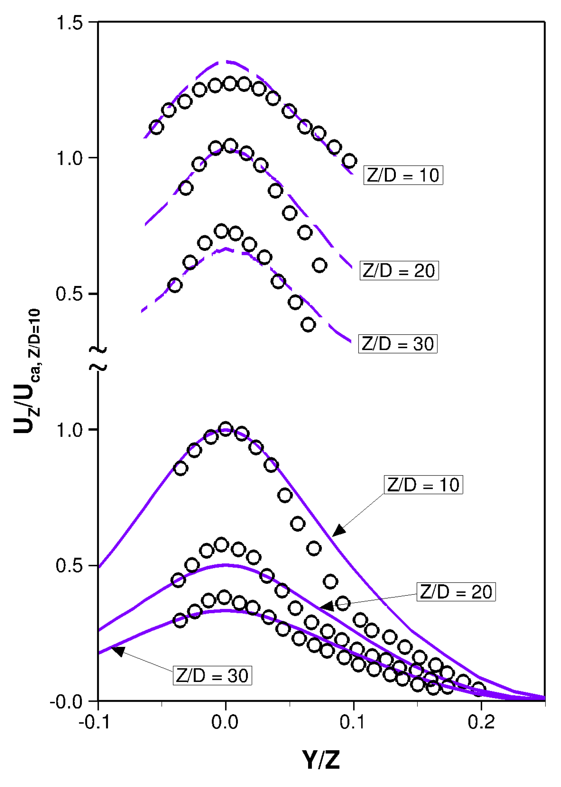
The validation of the simulation results was conducted by comparing the experimental normalized axial velocity observations reported by Fleckhaus et al. [15]. They used glass beads with properties of , and with a mass loading ratio of 0.3. Figure 2 presents the predicted velocity of the disperse phase at three locations ( and ) along the centerline. The resulting values compare well with the published experimental data in [15]. The results were normalized by the maximum velocity of continuum phases along section . In Figure 2, the results of simulations are compared with the experimental data from [15], which are in a very good agreement. In Figure 2, dispersed and continuum phase are indicated using dashed and solid lines, respectively. Two million parcels are injected to reduce the statics errors to an acceptable value to obtain the graphs of the disperse phase for each case. Nevertheless, perturbations can be seen in the diagrams. These high-frequency oscillations are omitted using a high pass filter after applying Fourier transform in the frequency domain. There are different approaches such as filtering, parcel-number-density control algorithms which are used to achieve numerically convergent solutions in Eulerian–Lagrangian (EL) simulations [21,28,29]. As it is shown in Figure 2, the decay rate obtained from the simulation results for the continuum phase is higher than those obtained from the experimental data. It can be seen that at larger distances from the nozzle, the normalized velocity of the dispersed phase falls below that which is presented by the experimental data. In the case of the Lagrangian phase, the results show overestimated value for section Z⁄D = 10. However, the simulation results at Z⁄D = 20, 30 shows lower value comparing experimental result, due to a higher decay rate. The numerical dissipation can be a reason for the high decay rate of velocity profiles.
5. Results and Discussion
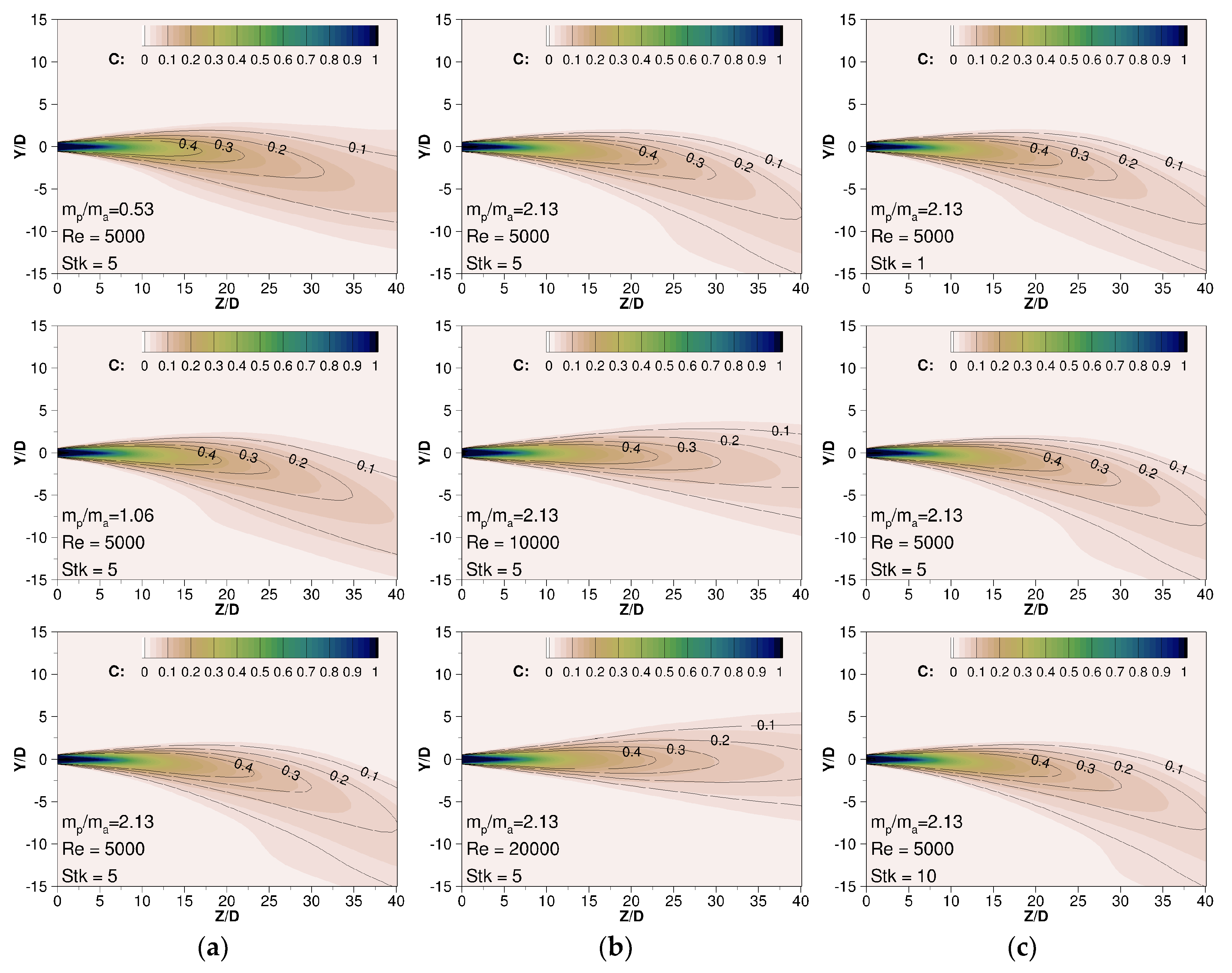
In the present study, to investigate the influence of the presence of particles on the jet motion direction, a passive scalar as a tracer of concentration of the continuum phase is injected at the nozzle (jet) entrance. This scalar shows the concentration of a scalar tracer which comes out from the jet. Figure 3, from left to right, demonstrates the influence of mass loading, Reynolds number of the jet and Stokes number of the particles on the concentration distribution of the continuous phase and distribution of the axial velocity of the continuum phase, respectively. The jet velocity profile at the top of the jet is quite similar to that of the spread of the jet tracer. In comparison, at the bottom of the jet, where the particles leave this region of the jet, the rate of spread of the jet tracer is higher. The amplitude of the velocity shows a general form of the jet. However, it cannot present the distribution of the flow rather the extension of the momentum in the calculation domain. In this study, one aim is to determine the influence of the particles on the mass motion of the continuous phase. The contour of the velocity is shown as line profiles in Figure 3. Velocity, unlike concentration, does not accumulate at one point. This is due to the presence of convection inherent in locations where there is flow velocity. Moreover, velocity does not accumulate over time at any given point in the domain as a result of the dissipation. Using the contour of concentration, it has been shown that the released flow is concentrated at the bottom of the main trajectory line of the jet. This is of critical importance in waste disposition, where it may contain particles that should not be accumulated at one point.
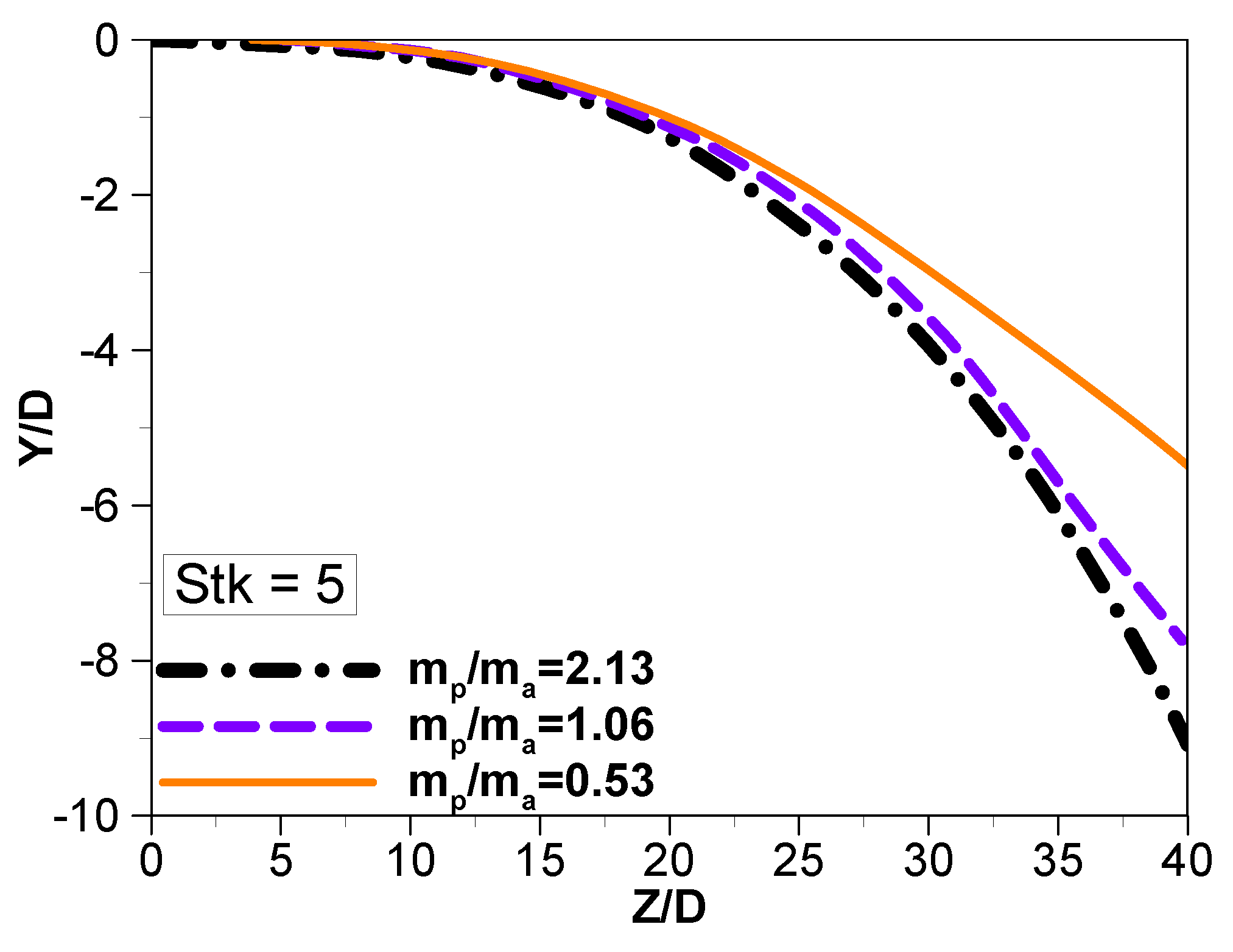
This lies in the fact that the downward motion of the particles changes the momentum direction downward and deviates from the original path. Moreover, it counteracts the influence of the ambient entrainment toward the jet in the lower region of the jet, which increases the rate of spread of the jet tracer as the particles leave the jet. In Figure 4, the path of the motion of the continuum phase is drawn by connecting the maximum points of the tracer. Furthermore, the rate of spread of the jet tracer at the bottom of the jet increases with growth in mass loading. Initially, the particles and jet have the same velocity. However, after a while, the particles tend to push jet in the downward direction as a result of gravitational force. It can be said that, gradually, the particles have more effects on the jet streamline. At higher Stokes number, the accumulation of continuum phase occurs at larger distance from the nozzle. This is due to the presence of larger particles, having a lower area/volume ratio, resulting in smaller drag forces per volume. It can be said that particles with a larger diameter and higher stokes number will decay their momentum at larger distances from the nozzle. On the other hand, particles will exit the jet and transfer their downward velocity, as a result of gravity, to the surrounding fluid. Due to this, smaller particles can transfer more downward momentum to the fluid. As a result, jets laden with smaller particles will have a downward trend. Initially (Z/D = 0), the particles and jet have the same velocity. However, after a while, the particles tend to push jet in the downward direction as a result of gravitational force. It can be said that, gradually, the particles have more effects on the jet streamline. The decay rate of the axial velocity and the concentration of the continuum phase (tracer) in the direction of the jet (Figure 4) are depicted in Figure 5.
The results reveal that the impact of mass loading on the gas-phase concentration decay rate is considerably low. However, the decay rate of the axial velocity decreases with a rise in mass loading. The total momentum of the particle laden-jet becomes larger, with an increase in mass loading. Meanwhile, the velocity of the gas-phase, which is deteriorated and scattered, is compensated by the transfer of the momentum from particles to the gas.
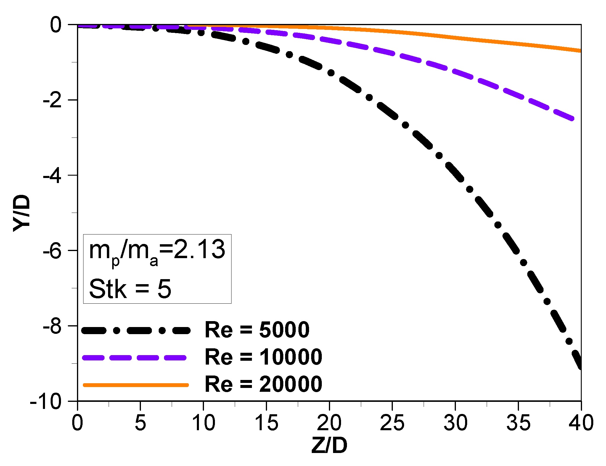
Figure 3b and Figure 6 indicate that the deflection of the jet path is diminished by increasing the Reynolds number. This is due to an increase in jet momentum, while the gravitational force is not strong enough to deflect the jet trajectory. Moreover, the increase in jet velocity enhances the ambient entrainment, and the initiated radial velocity toward the jet hinders the release of the particles from the jet, which leads to a reduction in the spread rate. However, by decreasing the Reynolds number, the gravitational force can deviate the particles from the jet and shift the momentum to the ambient, giving rise to the decay rate of the axial velocity.
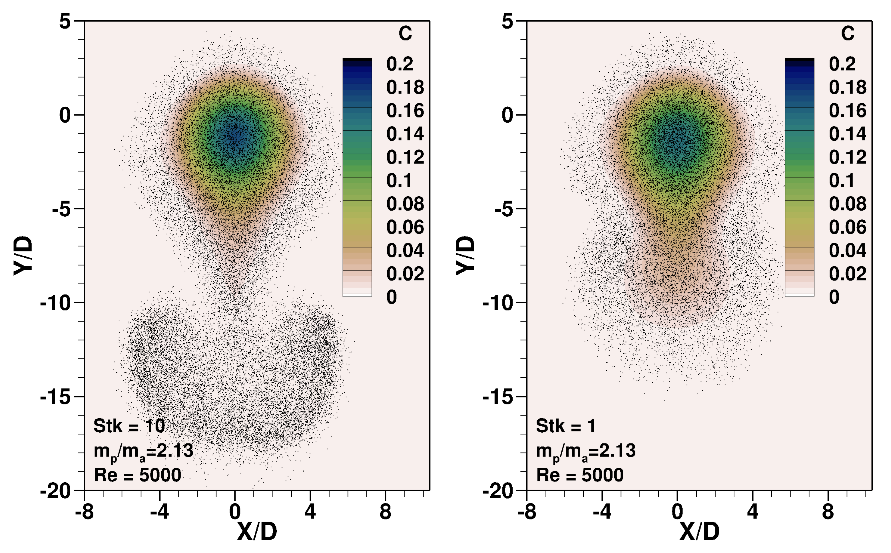
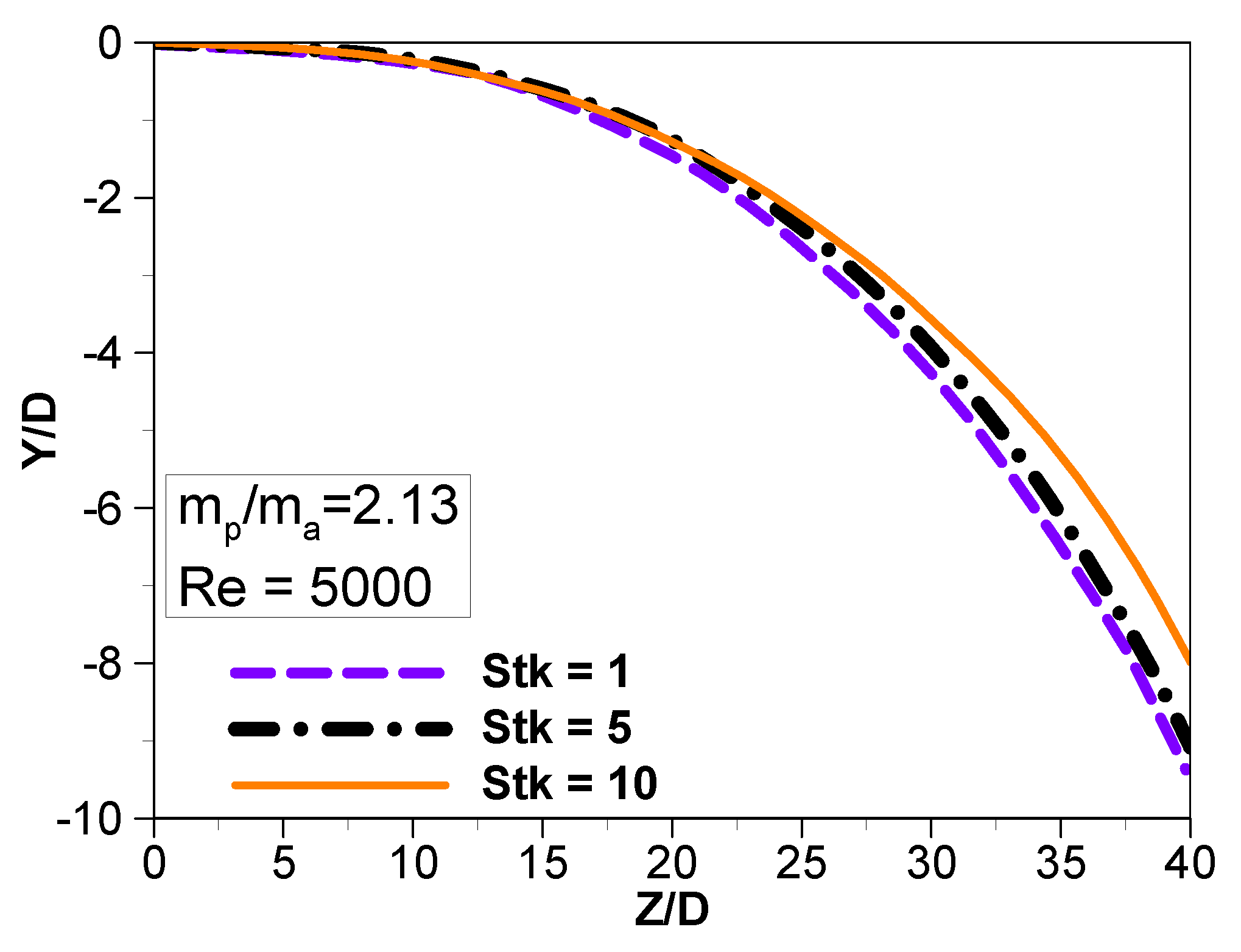
Figure 3c shows that the spread of the jet tracer suddenly increases at the bottom of the jet. Considering Figure 7, this increase is due to the particles being released from the jet bottom. These particles drag down part of the continuous phase, which increases the depth of the continuous phase penetration beneath the jet. Moreover, it can be seen that particles move out of the jet faster and farther away due to the Stokes number rise. This leads to an increase in the depth of the continuous phase beneath the jet. Nevertheless, since the coupling amongst particles is weaker for higher Stokes number, they cannot deflect the jet trajectory and gradually depart the jet. In comparison, as Figure 8 demonstrates, particles with stronger coupling, due to lower Stokes number, remain in the jet resulting in jet deflection.
6. Conclusions
The motion of a particle-laden jet was simulated with the particle size of and density of . The direction of the motion of the jet was traced by adding a tracer to the solver. The simulation results were validated with available experimental data. Moreover, the impacts of Stokes numbers, mass loading ratio and Reynolds number were studied. The following statements can be inferred from the results:
The total momentum of the particle-laden jet becomes larger with an increase in mass loading and the velocity of the gas-phase, which is deteriorated and scattered, is compensated by the transfer of the momentum from particles to the gas.
With a decrease in Reynolds number, the gravity force results in deflection of the particles from the jet and shifts the momentum to the ambient, giving rise to the decay rate of the axial velocity.
As the Stokes number increases, the particles leave the jet faster and are therefore less capable of bending the continuous phase trajectory of the jet. However, particles with lower Stokes numbers have less slip velocity than the continuous phase and their longer presence in the jet results in greater gravitational force effects and consequently more jet deflection.
Author Contributions
Conceptualization, A.T., and T.T.; methodology, H.T., T.T. and A.T.; software, H.T.; validation, H.T., and T.T.; formal analysis, A.T., H.T. and T.T.; writing—original draft preparation, T.T.; writing—review and editing, A.T.; supervision, A.T.; All authors have read and agreed to the published version of the manuscript.
Funding
This research received no external funding.
Acknowledgments
The authors would like to appreciate Compute Canada for its technical support and to provide computational resources.
Conflicts of Interest
The authors declare no conflict of interest.
Nomenclature
| QUANTITY | SYMBOL |
| Density | |
| Time | |
| Velocity | |
| velocity vector in ith direction | |
| Pressure | |
| Gravity | |
| Gravity in direction | |
| Stress tensor | |
| Drag Force (kg m/s2) | |
| Momentum Source term | |
| Viscosity | |
| turbulent viscosity | |
| Mass | |
| Diameter (m) | |
| Computational weight | |
| Reynolds number | |
| Stokes number | |
| fluctuating velocity | |
| particle eddy crossing time scale | |
| Viscosity | |
| Normally distributed random number | |
| Isotropic Lagrangian turbulence time scale | |
| Characteristic time of a Lagrangian phase | |
| Eulerian length scale | |
| Characteristic time of a continuum phase | |
| Schmidt number | |
| turbulent Schmidt number | |
| Relative velocity | |
| Particle relaxation time (s) | |
| Instantaneous velocity | |
| Particle Reynolds number | |
| indices of x, y, z-direction | i |
References
- The effects of crossing trajectories on the dispersion of particles in a turbulent flow. J. Fluid Mech. 1983, 136, 31–62. [CrossRef]
- Fan, J.; Zhao, H.; Jin, J. Two-phase velocity measurement in particle-laden coaxial jets. Chem. Eng. J. Biochem Eng. J. 1996, 63, 11–17. [Google Scholar] [CrossRef]
- Eaton, J.K. Structure of a particle-laden round jet. J. Fluid Mech. 1992, 236, 217–257. [Google Scholar]
- Heitor, M.V.; Moreira, A.L.N. On the analysis of turbulent transport processes in nonreacting multijet burner flows. Exp. Fluids 1992, 189, 179–189. [Google Scholar] [CrossRef]
- Puttinger, S.; Holzinger, G.; Pirker, S. Investigation of highly laden particle jet dispersion by the use of a high-speed camera and parameter-independent image analysis. Powder Technol. 2013, 234, 46–57. [Google Scholar] [CrossRef]
- Series, S. Turbulent Particle-Laden Gas Flows; Springer: Berlin, Germany, 2007. [Google Scholar] [CrossRef] [Green Version]
- Wang, X.; Zheng, X.; Wang, P. Direct numerical simulation of particle-laden plane turbulent wall jet and the influence of Stokes number. Int. J. Multiph. Flow 2017, 92, 82–92. [Google Scholar] [CrossRef]
- Patro, P.; Dash, S.K. Computations of particle-laden turbulent jet flows based on eulerian model. J. Fluids Eng. 2013, 136, 011301. [Google Scholar] [CrossRef]
- Jebakumar, A.S.; Abraham, J. Comparison of the structure of computed and measured particle-laden jets for a wide range of Stokes numbers. Int. J. Heat Mass Transf. 2016, 97, 779–786. [Google Scholar] [CrossRef]
- Luo, K.; Gui, N.; Fan, J.; Cen, K. Direct numerical simulation of a two-phase three-dimensional planar jet. Int. J. Heat Mass Transf. 2013, 64, 155–161. [Google Scholar] [CrossRef]
- Lee, J.; Lee, C. Modification of particle-laden near-wall turbulence: Effect of stokes number. Phys. Fluids 2015, 27, 1–28. [Google Scholar] [CrossRef] [Green Version]
- Crowe, C.T.; Schwarzkopf, J.D.; Sommerfeld, M.; Tsuji, Y. Multiphase Flows with Droplets and Particles; CRC Press: Boca Raton, FL, USA, 2011. [Google Scholar] [CrossRef]
- Kazemi, S.; Adib, M.; Amani, E. Numerical study of advanced dispersion models in particle-laden swirling flows. Int. J. Multiph. Flow 2018, 101, 167–185. [Google Scholar] [CrossRef]
- Xu, J.; Mohan, M.; Ghahramani, E.; Nilsson, H. Modification of Stochastic Model in Lagrangian Tracking Method; Chalmers University of Technology: Göteborg, Sweden, 2016. [Google Scholar]
- Fleckhaus, D.; Hishida, K.; Maeda, M. Effect of laden solid particles on the turbulent flow structure of a round free jet. Exp. Fluids 2000, 28, 96. [Google Scholar] [CrossRef]
- Abessi, O.; Roberts, P.J.W. Rosette diffusers for dense effluents in flowing currents. J. Hydraul. Eng. 2018, 144. [Google Scholar] [CrossRef]
- Yan, X.; Mohammadian, A.; Chen, X. Three-dimensional numerical simulations of Buoyant Jets discharged from a Rosette-type multiport diffuser. J. Mar. Sci. Eng. 2019, 7, 409. [Google Scholar] [CrossRef] [Green Version]
- Pope, S.B. Turbulent Flows. Meas. Sci. Technol. 2001, 12, 11. [Google Scholar] [CrossRef]
- Menter, F.R. Two-equation eddy-viscosity turbulence models for engineering applications. AIAA J. 1994, 32, 1598–1605. [Google Scholar] [CrossRef] [Green Version]
- Février, P.; Simonin, O. Statistical and continuum modelling of turbulent reactive particulate flows Part II: Application of a two-phase second-moment transport model for prediction of turbulent gas-particle flows. Lect. Ser. Kareman Inst. Fluid Dyn. 2000, 6, E1–E24. [Google Scholar]
- Tofighian, H.; Amani, E.; Saffar-Avval, M. Parcel-number-density control algorithms for the efficient simulation of particle-laden two-phase flows. J. Comput. Phys. 2019, 387, 569–588. [Google Scholar] [CrossRef]
- Jayaraju, S.T.; Sathiah, P.; Roelofs, F.; Dehbi, A. RANS modeling for particle transport and deposition in turbulent duct flows: Near wall model uncertainties. Nucl. Eng. Des. 2015, 289, 60–72. [Google Scholar] [CrossRef]
- Gao, N.; Niu, J.; He, Q.; Zhu, T.; Wu, J. Using RANS turbulence models and Lagrangian approach to predict particle deposition in turbulent channel flows. Build. Environ. 2012, 48, 206–214. [Google Scholar] [CrossRef]
- Focht, E. A Method for Unstructured Mesh-to-Mesh Interpolation, DTIC Doc. 2008. Available online: http://www.dtic.mil/cgi-bin/GetTRDoc?AD=ADA319658APPROVED (accessed on 7 April 2020).
- Moukalled, F.; Mangani, L.; Darwish, M. The Finite Volume Method in Computational Fluid Dynamics—An Advanced Introduction with OpenFOAM and Matlab; Springer: Berlin, Germany, 2016. [Google Scholar] [CrossRef] [Green Version]
- Swebyi, P.K. High resolution schemes using flux limiters for hyperbolic conservation laws. SIAM J. Numer. Anal. 1984, 21, 995–1011. [Google Scholar] [CrossRef]
- Macpherson, G.B.; Nordin, N.; Weller, H.G. Particle tracking in unstructured, arbitrary polyhedral meshes for use in CFD and molecular dynamics. Commun. Numer. Methods. Eng. 2009, 25, 263–273. [Google Scholar] [CrossRef]
- Graham, D.I.; Moyeed, R.A. How many particles for my Lagrangian simulations ? Power Technol. 2002, 125, 179–186. [Google Scholar] [CrossRef]
- Messa, G.V.; Malavasi, S. The effect of sub-models and parameterizations in the simulation of abrasive jet impingement tests. Wear 2016, 370, 59–72. [Google Scholar] [CrossRef]
Figure 1.
Computational domain and mesh structure.

Figure 2.
The comparison between normalized axial velocities resulted from simulation and experimental data [15]. Dashed line is the disperse phase, the solid line is continuum phase and symbols are experimental data observed by [15].

Figure 3.
The contours of jet tracer scalar: (a) The left side is for different mass loading ratios at Re = 5000, Stk = 5. (b) The middle one is for different Reynolds numbers at m_p⁄m_a = 2.13, Stk = 5. (c) The right side is for different Stokes number at m p⁄m_a = 2.13, Re = 5000. The lines represent the velocity contour.

Figure 4.
The effect of mass loading ratio on the trajectory of the gas-phase jet at Re = 5000.

Figure 5.
The effect of mass loading ratio on the velocity and tracer concentration decay rate on the trajectory of the gas-phase jet.
Figure 5.
The effect of mass loading ratio on the velocity and tracer concentration decay rate on the trajectory of the gas-phase jet.

Figure 6.
The effect of Reynolds number on the trajectory of the particle-laden jet.

Figure 7.
The counter of the continuous phase and position of the particles in Z/D = 20 section with Stokes number 1 and 10 from right to left, respectively.
Figure 7.
The counter of the continuous phase and position of the particles in Z/D = 20 section with Stokes number 1 and 10 from right to left, respectively.

Figure 8.
The effect of Stokes number on the trajectory of particle-laden jet.


Table 1.
The parameters of four different cases.
| Mass Loading | Computational Weight of Parcels | ||
|---|---|---|---|
| 0.53 | 5 | 5000 | 40 |
| 1.06 | 5 | 5000 | 80 |
| 2.13 | 5 | 5000 | 160 |
| 2.13 | 5 | 10,000 | 160 |
| 2.13 | 5 | 20,000 | 160 |
| 2.13 | 1 | 5000 | 17, 20 |
| 2.13 | 10 | 5000 | 55 |
© 2020 by the authors. Licensee MDPI, Basel, Switzerland. This article is an open access article distributed under the terms and conditions of the Creative Commons Attribution (CC BY) license (http://creativecommons.org/licenses/by/4.0/).
Share and Cite
MDPI and ACS Style
Tavangar, T.; Tofighian, H.; Tarokh, A. Investigation of the Horizontal Motion of Particle-Laden Jets. Computation 2020, 8, 23. https://0-doi-org.brum.beds.ac.uk/10.3390/computation8020023
AMA Style
Tavangar T, Tofighian H, Tarokh A. Investigation of the Horizontal Motion of Particle-Laden Jets. Computation. 2020; 8(2):23. https://0-doi-org.brum.beds.ac.uk/10.3390/computation8020023
Chicago/Turabian StyleTavangar, Tooran, Hesam Tofighian, and Ali Tarokh. 2020. "Investigation of the Horizontal Motion of Particle-Laden Jets" Computation 8, no. 2: 23. https://0-doi-org.brum.beds.ac.uk/10.3390/computation8020023
Note that from the first issue of 2016, this journal uses article numbers instead of page numbers. See further details here.