1. Introduction
Robotic science and technology are playing increasingly an essential role in human society, and they are helping and improving the quality of our lives in many different ways, from transportation to robotic surgery [
1,
2,
3,
4]. Robots can be designed to perform complex tasks to reduce the amount of human involvement, so that automation of the process becomes possible. However, robots may break down, and the cost of its repair or replacement can be very high. Therefore, one may consider replacing sophisticated robots with many simpler robots that are less complex but which can still perform tasks of the complex robots [
5]. The advantage of using swarms of simpler robots is that, even if some robots get damage the tasks can still be completed, as there is redundancy built into to the swarm. Furthermore, in achieving some tasks, a swarm of robots may be more flexible than a single complex robot. Moreover, by sharing their knowledge and learning experience from each other within a swarm, the robots may learn faster how to perform some tasks in dynamically changing environments. Given these attributes a swarm of robots may perform some tasks more reliably, effectively and efficiently than a single complex robot [
6,
7,
8]. These characteristics of swarm robotics motivated us to conduct a modelling and simulation study on cognitive agents learning to cross a cellular automaton (CA)-based highway. These cognitive agents can be considered as an abstraction of a swarm of simple robots, however, they are general enough so that, they may be considered as an abstraction of an autonomous vehicle learning to cross a unidirectional highway. The cognitive agents have the intelligence of learning from each other and complex traffic environment. The study of their decision outcomes of crossing the highway can help to understand how experimental setups of input factors influence the results of the cognitive agents’ decisions. The detailed description of the considered mathematical model and its software implementation can be found in [
9,
10,
11]. Within the simulation process, the goal of cognitive agents is to learn to cross a CA-based highway, and different types of decision outcomes are observed and recorded as simulation progresses. Therefore, there are many data files generated by a large number of different experimental setups of input factors, which are the outputs of the simulation model and which are analyzed in this paper. The studies of [
12,
13,
14] mainly have focused on the mathematical modelling and its software implementation, but not on the analysis of the simulation data for a better understanding of the relationships between input factors and the output variables, which is addressed in this paper.
The construction of mathematical models and the design of their computer simulations must incorporate many factors of the modelled systems to capture and control properly their dynamics and performance. To understand “cause and effect” of input factors on the experimental outcomes one should apply various statistical methods to analyze the simulation data. Since the presented study is an experimental one, by modelling the relationships between the input factors and the output variables, we can identify the causal relationships among them. Our previous study in [
15] has demonstrated that there is a significant relationship between the input factors and output variables in the simulation data of cognitive agents learning to cross a CA-based highway. All of these have motivated our predictive modelling of the data coming from the considered simulations. We aim to design a predictive model which can better explain the uncertainty of the simulation model as well as to establish a mathematical relationship between the input factors and output variables of the simulation model. Due to the potential existence of non-linear relationships observed between input factors and output variables in many complex systems’ data [
16], we propose an approach of using artificial neural networks (ANNs) to model our simulation data. ANNs are sophisticated computational models having their strength due to their ability of approximating the non-linear relationships between input factors and output variables and due to the joint effects of weights and activation functions [
17,
18]. ANN models have a wide range of applications in many fields, including both regression and classification problems. In [
19], artificial neural networks were used to make predictions and forecasting of quantitative characteristics of water bodies. In [
20], both ANN and support vector machines were used to detect potential system intrusions using data from the DARPA 1998 Intrusion Detection Evaluation Program at MIT’s Lincoln Labs. More recently, in [
21], ANN was used for the diagnosis of Sleep Apnea Syndrome. In [
22], ANNs were combined with response surface techniques for modelling and optimization of biosorption to study the interaction effects of process variables. A similar idea was also applied in [
23] to predict the wetting phenomena for synthetic wastewater treatment. In [
24], ANN was used to model the Pleurotus sp. cultivation process, and the study showed that ANN modelling outperformed other mathematical modelling techniques that were considered in their work. The success of these applications using ANN may be due to the fact that ANN is capable of explaining the non-linear data patterns.
The main limitation of ANNs is the difficulty in explaining the relationships between input factors and output variables, unlike linear or generalized linear models, which can be explained by evaluating the model coefficients. Fortunately, one can measure a variable importance by using the weight values obtained from a ANN, and there are specific algorithms or functions, including Garson algorithm [
25] and Olden function [
26], which can be applied. The Garson algorithm computes the summed product of absolute weight values of input-hidden and hidden-output connections, which is normalized in such a way that the final computed value is between 0 and 1, while the Olden function simply computes the summed product of weight values without the normalization. Furthermore, the Olden function can be applied to ANN models with multiple hidden layers, while the Garson algorithm works for only the single hidden layer. Because of the flexibility of the Olden function, in this work, we apply this function to evaluate the importance of input variables. The obtained measures of importance of the input factors help us to better understand the impact of our experimental factors on the decision outcomes of cognitive agents, when learning to cross the CA-based highway.
To demonstrate that the ANN is a promising method in statistical modelling of the simulation data of a complex system model like ours, we have compared the proposed ANN models performance with other traditional approaches, like multiple linear regression (MLR) and generalized linear models (GLM). Our comparison illustrates the limitations of linear and generalized linear models in capturing non-linear relationships of complex simulation data. In traditional analysis of designed experiments, linear models are the ones which are most often considered. Within our study, we demonstrate the potential usefulness of using non-linear regression models to analyze data from designed experiments. We evaluate the variable importance using the Olden function [
26] to investigate the impact of the input factors on the response variables. The novelty of our work consists of the fact that, we have combined a simulation study of our mathematical model with data analysis using sophisticated statistical approaches. The significance of our work is in showing that this approach provides an improved insight in understanding performance and dynamics of simulation models of complex systems. This paper is organized as follows. In
Section 2, the simulation model used for generating the experimental data is briefly described. In
Section 3, we discuss the statistical modelling methods, like ANNs, generalized linear models and multiple linear regression models. In
Section 4, analysis of simulation data and summary of the main results are presented. In
Section 5, we conclude our findings and provide further comments.
2. Simulation Model of Autonomous Agents Learning to cross CA Based Highway
In this section, we briefly introduce the simulation model of cognitive agents learning to cross a CA-based highway. The reader is referred to [
9,
10,
11] for a more detailed description of the simulation model as well as the previous results of statistical analysis of the simulation data. This simulation model consists of three main components, the highway, vehicles and cognitive agents, respectively, and the agents’ process of learning. The real highway is discretized and its model consists of many cells, each representing 7.5 m of the highway length. Each vehicle moves from one cell to another one depending on its speed. In the simulator the number of lanes and the length of the highway are initialized before starting the simulation runs. In our simulations we consider a unidirectional single lane subset of the highway consisting of 120 cells. Each cell of the highway can be only in one of the two states: occupied or not. If a vehicle or an agent is present in a cell, then the cell is occupied. Otherwise, it is empty. Furthermore, an agent and a vehicle are not allowed to occupy the same cell simultaneously. If an incoming vehicle moves into a cell occupied by an active agent (i.e., the one attempting to cross the highway) or to a cell located past the cell occupied by the active agent, then it is considered that the active agent was hit and killed, and this agent is removed immediately from the highway. At the beginning of the highway, a vehicle is generated with Car Creation Probability (CCP), at each time step. The process of moving vehicles follows the modified Nagel-Schreckenberg CA traffic model [
27]. The moving behaviours of the vehicles are controlled by the Random Deceleration (RD) parameter, values of which can be 0 or 1. If RD = 1, then the vehicles will additionally randomly decelerate with the probability 0.5. When RD = 0, then they do not randomly decelerate.
The only goal of our cognitive agents is to cross the highway successfully, i.e., without being hit by incoming vehicles. The cognitive agents are generated on the same side of the highway at a certain crossing point, in our case located at the cell 60 from the beginning of the highway. In the simulation, there is a parameter called Horizontal Movement (HM). When HM is equal to 0, then the cognitive agents cannot change their crossing point, i.e., move horizontally in either direction. So they can only wait at the crossing point or they can try to cross the highway. If HM is equal to 1, and the active agents decide not to cross the highway, then they can stay at their crossing points, or they can move randomly one cell in either direction. When crossing the highway, active agents experience various intensities of their Fear (i.e., propensity to risk avoidance) and Desire (i.e., propensity to risk taking), which influence their decision-making process. In the simulation model, these parameters can take values from the set {0, 0.25, 0.5, 0.75, 1.0}. The cognitive agents learn from the experience of other agents who attempted to cross the highway earlier at their crossing points. Based on this experience, each agent attempting to cross makes its own decision, and the result of this decision is recorded in the Knowledge-Based (KB) table. The KB table is updated each time an active agent makes its decision for use by the next active agent in its decision-making process. The Knowledge Base Transfer (KBT) parameter in this work is a binary variable taking value 0 or 1. If KBT = 0, then the Knowledge Base Transfer does not occur. If KBT = 1, then the KB table at the end of the simulation in a less dense traffic environment is transferred to the agents at the beginning of the simulation in an immediately denser traffic environment. The entries of the KB table record, for each incoming vehicle an estimated distance (close, medium-far, far, out of horizon of vision) and an estimated speed (slow, medium, fast, very fast), the active agents’ decisions successes or failures in crossing the highway, i.e., at each time t they display the numbers of the active agents’ correct crossing decisions (CCDs), incorrect crossing decisions (ICDs), correct waiting decisions (CWDs), incorrect waiting decisions (IWDs), which the active agents made for each observed pair of an estimated distance and an estimated speed from the beginning of the simulation run [
28,
29]. Each active agent uses the information contained in the KB table in its decision-making process when it attempts to cross the highway.
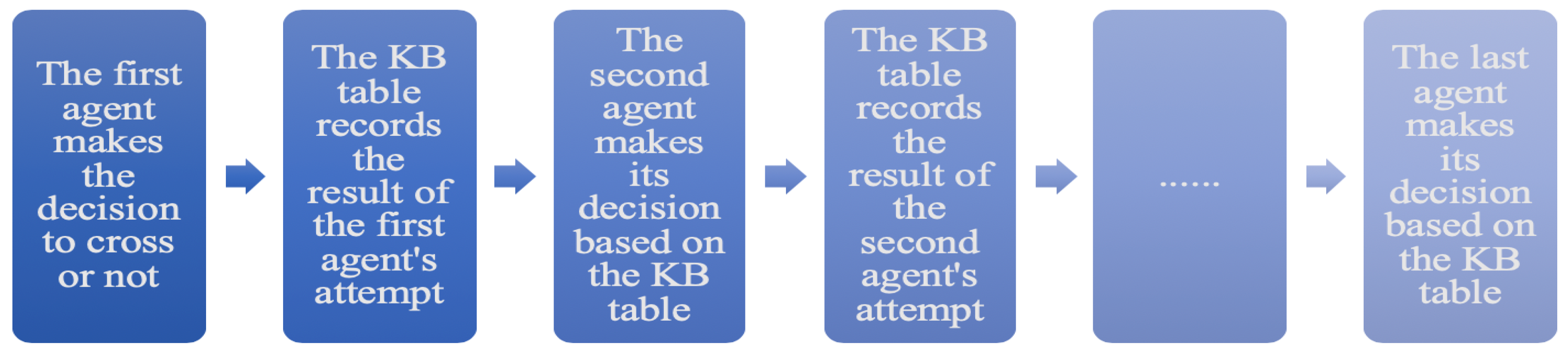
As the simulation progresses and the active agents make crossing or waiting decisions, the record of the KB table is updated. The illustration of the update of the KB table is given in
Figure 1. Next, at each time
t, the updated record is used to calculate the values of an active agent decision-making formula. In this work, for illustrative purposes, we analyze only the simulation data of the agents using the Crossing-and-Waiting Based Decision Formula (cwDF) [
28,
29,
30], and we determine optimal numbers of clusters using these data. For the description of another decision-making formula called Crossing-Based Decision Formula (cDF) the reader is referred to [
28,
29,
30]. The decision-making formula cwDF is based on the numbers of all four decisions, i.e., CCDs, ICDs, CWDs, IWDs, recorded in the KB table. At each time
t, for an observed distance of an incoming vehicle and its estimated speed, based on the numbers in the corresponding entry of the KB table, the value of cwDF is calculated. Next, this value is compared with an active agent’s threshold, which is based on the values of its Fear and Desire factors. If the calculated value of the decision-making formula cwDF is greater than the threshold value, then the active agent attempts to cross the highway. If it is not, then the active agent waits, and if the simulation setup allows, the active agent may move to one of the neighbouring crossing points. If HM = 0, then the active agent does not change its crossing point. After the vehicle passes, the active agent decision is assessed as being correct or incorrect, and the record is updated in the KB table [
28,
29,
30].
We consider the following response variables: CCD, ICD, CWD, IWD, which are, respectively, the numbers of CCDs, ICDs, CWDs and ICDs. For each simulation repeat, these numbers are obtained by summing up over the entries of the KB table the respective numbers at the simulation end. The values of the response variables are affected by the various factors and their levels. In our simulations, each the factors CCP, Fear and Desire, has five levels, and the factors KBT, RD and HM are binary variables [
28,
29,
30]. For each setup of the factors’ values we run each simulation for 1511 time steps and we repeat the simulation 30 times for different seed values of the random number generators.
3. Methods
Modelling and simulation are only the initial steps in the investigation of complex systems performance and dynamics. To discover how various factors, their levels and their interactions affect these systems performance and dynamics one must use either dynamical systems and bifurcation theory approach, which is not always possible, or one must investigate simulation data by using various statistical methods. In [
15], we have investigated the interconnections between the experimental setups and the considered output variables CCD, ICD, CWD, and IWD, using canonical correlation analysis (CCA). The obtained results, discussed in [
15], provide us with statistical evidence of existence of the mathematical relationships between input factors and output variables. Furthermore, in [
15], we conducted a regression tree analysis of studying the effects of the input factors on the output variables. However, the obtained results only displayed the qualitative effects. In this work, we consider a predictive modelling approach via ANNs. We try to model the functionality between the decision outcomes of active agents and the input factors of the simulation experiments. In this section, we briefly discuss the proposed methodology and address some connections between ANNs and the traditional modelling methods.
First, let us discuss the case of ANN with two hidden layers. Suppose that in an ANN model, there are
D input factors
,
, …,
, and
hidden neurons
,
,
…,
in the first hidden layer. In the first hidden layer, a neuron
can be defined as
where
=
. Thus, each activation
is composed of the linear combination of the input variables
, their weights
and the bias
. The superscript (1) in the weights indicates that components correspond the first hidden layer. The function
is referred to as the activation function, which is usually differentiable and non-linear. Often, the activation function is chosen to be a sigmoidal function [
31].
Given a hidden neuron
of the first hidden layer, the resulting output neuron activation
for the second hidden layer can be written as
where
represent the weights,
are the bias terms and
represents the number of hidden neurons in the second hidden layer. The superscript (2) in the weights implies that the components correspond to the second hidden layer. The hidden neurons
,
,
…,
located in the second hidden layer, using the same activation function
, become
Note that, the activation function in the second hidden layer could be different from the first hidden layer. In classification problems using ANNs, the hidden neurons activations
are further transformed by using an appropriate activation function in order to calculate the outputs. The following logistic function is often employed as an activation function for the output layer
where
is the activation function applied to the last hidden layer to obtain the output layer. It can be a different activation function from
. Since we conduct a regression modelling, we do not apply this activation function. Therefore, the output of the
kth observation for a two hidden layers ANN becomes
where
are the results of the second hidden neurons from
kth observation input and
is the random noise term. Note that, the weight values and the bias terms are calculated by applying some gradient decent methods and a convergence criterion, such as the Backpropagation method.
Let us consider a more general case with multiple hidden layers. Denoting the input vector by
=
and assuming that the total number of hidden layers is
L, and that there are
hidden neurons
,
,
…,
in the
lth hidden layer, we can write the
hidden layer neurons as follows
for
, and
. If we further assume that the total number of observations for the input factors and output variables is
N, then the final output of the ANN for the
kth input vector of
x becomes
where
and
are, respectively, the weight values and the bias connecting the last hidden layer and the regression output, and
is the random noise term. Note that, each
is also a function of the weight values and biases from the previous layers. If we further denote the weight values of each hidden layer as a vector
, for
i = 1,…,
L and the bias vector at the last hidden layer as
, then the regression based on an artificial neural network model can be represented by the following regression equation
where
is the random noise. This is an implicit form of a non-linear regression model. In the case, that there is no hidden layer, the model in (
8) becomes the multiple linear regression (MLR) model, which can be explicitly written as follows:
where
are the model’s coefficients and
∼
. If we further allow the noise distribution to be the exponential family distribution instead of the normal distribution, then the regression model in (
9) becomes a generalized linear model (GLM) [
32]. For instance, if the observations are count data, like our simulation data, then the error function often is assumed to be Poisson distributed. Besides the extension from the normal distribution to the exponential family distributions, also, GLM has a component that allows us to transform a linear function of input factors (i.e., the mean response
in MLR) through introduction of a link function. The link function,
g, is used to establish the functional relationship between the mean response
and the linear combination of input variables. This relationship is defined as follows:
In the case of using GLM with Poisson as an error distribution, the link function is the logarithmic function. Thus, we can see that GLM is similar to an ANN without a hidden layer, but with the link function as an activation function. For more details on GLM methodology, we refer to [
32].
In this work, the input variables of ANN models are the factors CCP, Fear, Desire, KBT, RD and HM. The output variable for each ANN is one of the following response variables: CCD, ICD, CWD, IWD. Besides the model fitting using ANN, we also fit the data to both MLR and GLM. Akaike information criterion (AIC), Bayesian information criterion (BIC), root mean squared error (RMSE) and mean absolute deviation (MAD) are used to measure the model performance [
33,
34,
35]. The AIC and BIC are commonly used for a model selection, and the smaller the values of either AIC or BIC, the better is the model. Both AIC and BIC are calculated by using the likelihood function of the given data and the number of parameters in the model [
34]. The root mean squared error (RMSE) and the mean absolute deviation (MAD) are other two model error measures. The RMSE is the square root of the mean squared error (MSE) of a given model, while MAD is the average of the absolute values of deviations of the model [
35]. The model with the smaller values of these criteria indicates better goodness of fit.
4. Results
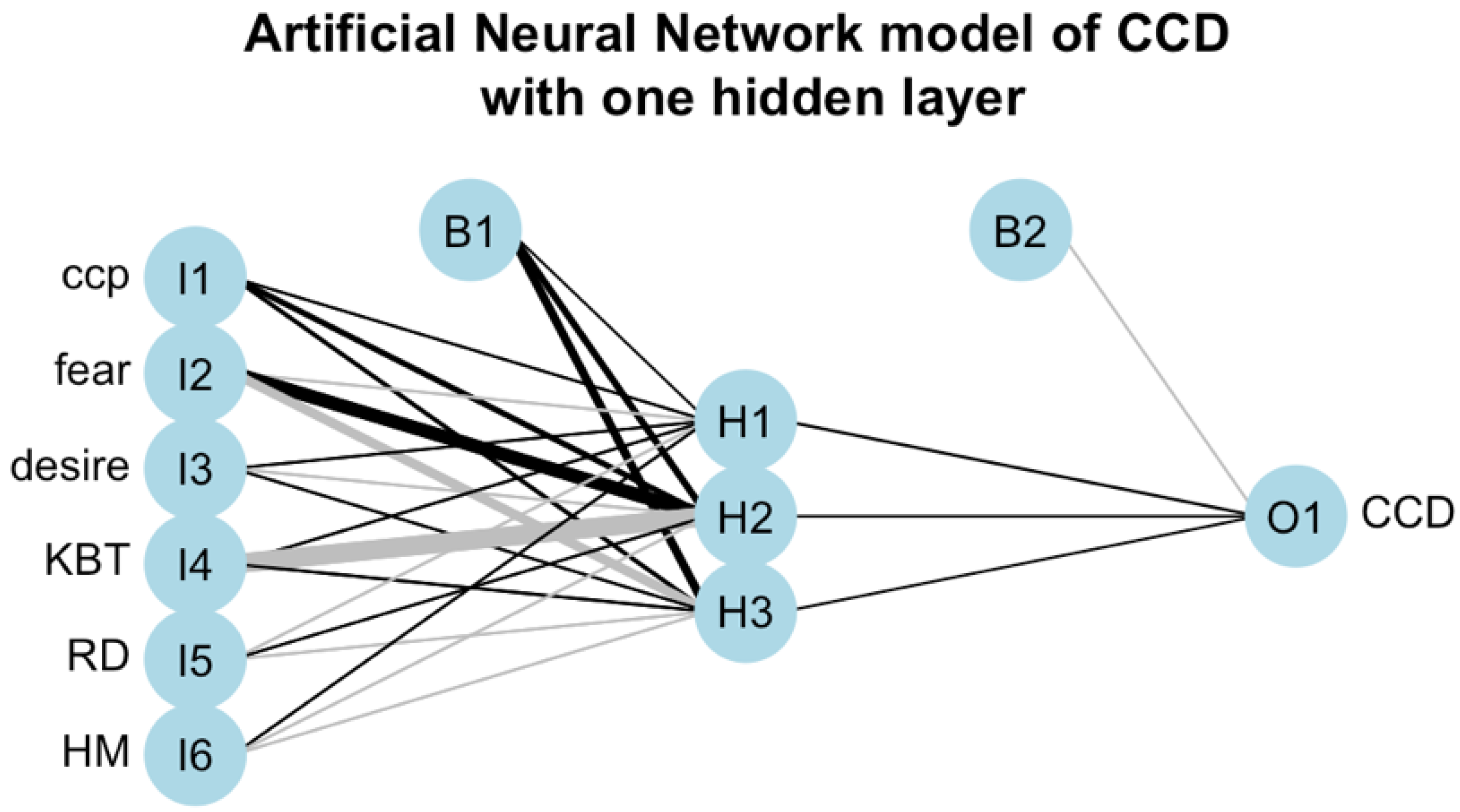
First, we illustrate an application of the ANN models as a regression technique using network graphs. The ANN used in this work is the feed-forward ANN, where the information flow is unidirectional, i.e., directly from the input layer to the output layer. The results in terms of the network graphs are displayed in
Figure 2 and
Figure 3. These two figures show the ANN models’ interpretation diagrams when the number of CCDs is used as the response variable. The number of correct crossing decisions of active agents is an essential metric measuring the success of learning in crossing the highway. We use this example as a case study of the effects of input factors on the output variables.
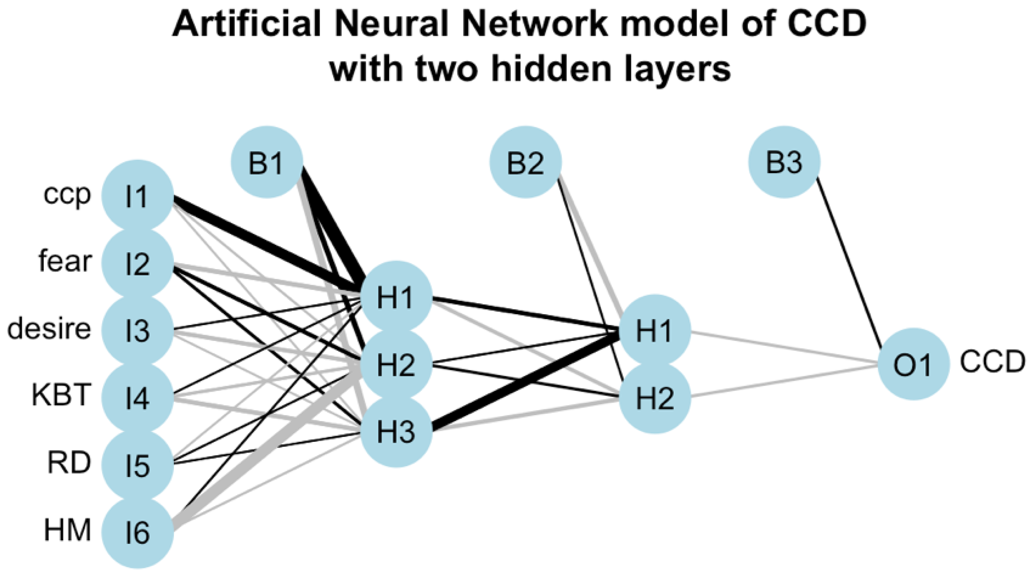
Figure 2 displays the ANN with one hidden layer with three neurons (i.e., ANN-3), and
Figure 3 displays the ANN with two hidden layers where three neurons are in the first layer and two neurons are in the second layer (i.e., ANN-3-2). These two typical ANN models are selected from other possible choices of ANN structures, as they are considered to be our best models based on our experiments. As we can see from both
Figure 2 and
Figure 3, the input layer contains the factors CCP, Fear, Desire, KBT, RD and HM, while the output layer contains the numbers of CCDs. When other decision outcome is used as a response variable, then the output layer contains either the numbers of ICDs, or the number of CWDs, or the number of IWDs. Each link in plots of the ANN models represents a connection from an input neuron to a neuron located in the next layer. To all connections between neurons are assigned the respective weights. The black links represent positive weight values between neurons, while the grey links represent negative weights. The thickness of each link represents graphically the absolute value of the magnitude of a weight, i.e., the strength of the connection. The thicker the link is, the bigger is the absolute value of a magnitude of the weight between the two neurons and the more influential is this connection. In our ANN models we use logistic functions as the activation functions between input-hidden and hidden-hidden layers and the identity function as the activation function for the output layer. All the statistical results of this paper were obtained using R and neuralnet package.
The result displayed in
Figure 2, i.e., for the ANN model with one hidden layer, shows that the input factor CCP contributes positively to all neurons of the hidden layer. This is not the case for the other factors, as their contributions are both positive and negative, and of various magnitudes, i.e., strengths. The positive contribution of the Fear factor to the neuron H2 of the hidden layer is much stronger than its negative contributions to the other two neurons of this layer. While the negative contribution of the KBT factor to the neuron H2 of the hidden layer is much stronger than its positive contributions to the other two neurons of this layer. The contributions of the other factors (i.e., Desire, RD, HM) are not as strong as of the factors Fear and KBT. Thus, the factors CCP, Fear and KBT are the most influential factors on the hidden layer. However, their individual impacts on the final output are not evident.
The result displayed in
Figure 3, i.e., for the ANN model with two hidden layers, shows that all the input factors contribute both positively and negatively, with various strengths, to all neurons of the first hidden layer. The strongest positive contribution comes from the input factor CCP and it is to the neuron H1 of the first hidden layer. The strongest negative contribution comes from the input factor HM and it is to the neuron H2 of the first hidden layer. In comparison with the result of
Figure 2, the input factors Fear and KBT are not as influential as they were in the case of the ANN model with one hidden layer. We notice on
Figure 3, that with various strengths, the neurons H1 and H3 contribute both positively and negatively to the neurons of the second hidden layer, while neuron H2 contributes only positively. The strongest positive contribution comes from the neuron H3 of the first hidden layer to the neuron H1 of the second hidden layer. In the case of the ANN model with two hidden layers it seems that the input factors CCP and HM, due to the strengths of their contributions to the fist hidden layer, are the most influential factors on the final output. However, their individual impacts are not evident.
In both
Figure 2 and
Figure 3, we see that, a positive or negative bias with different strength is added to each neuron of each hidden layer and to each output neuron. The bias term is added to the total sum of inputs as a threshold to shift the activation function to the left or the right [
36]. The bias terms can be interpreted as intercepts in the linear regression models, as discussed in
Section 3. Thus, it is crucial to have the bias terms included in the ANN models, when they are used as the linear regression models.
We further compare the performance of the ANN models for different decision types with different regression models. The obtained results are summarized in
Table 1,
Table 2,
Table 3 and
Table 4. From these results, we can see that, the corresponding AIC and BIC values of MLR and GLM models are much larger than those of the ANN models. This strongly suggests that the ANN models outperform the MLR and GLM models. However, the AIC and BIC values of MLR and GLM models are similar. Furthermore, the AIC and BIC values of the two ANN models are comparable to each other. Since both AIC and BIC are mainly determined by the models residual sum of squares (RSS), the large values of AIC and BIC imply that the RSS of MLR and of GLM are larger too, compared to the ANN models. In contrast, the RMSE and MAD values of the four models (i.e., LM, GLM, ANN-3, ANN-3-2) are more comparable as they are calculated using the square root of the mean squared errors and mean absolute errors, respectively. However, ANN models lead to smaller values of RMSE and MAD. Based on the performance measures we used, for each decision type, we see that, GLM is the worst performing model and MLR is the second-worst. The ANN models outperform the traditional models, especially for the ANN model with two hidden layers.
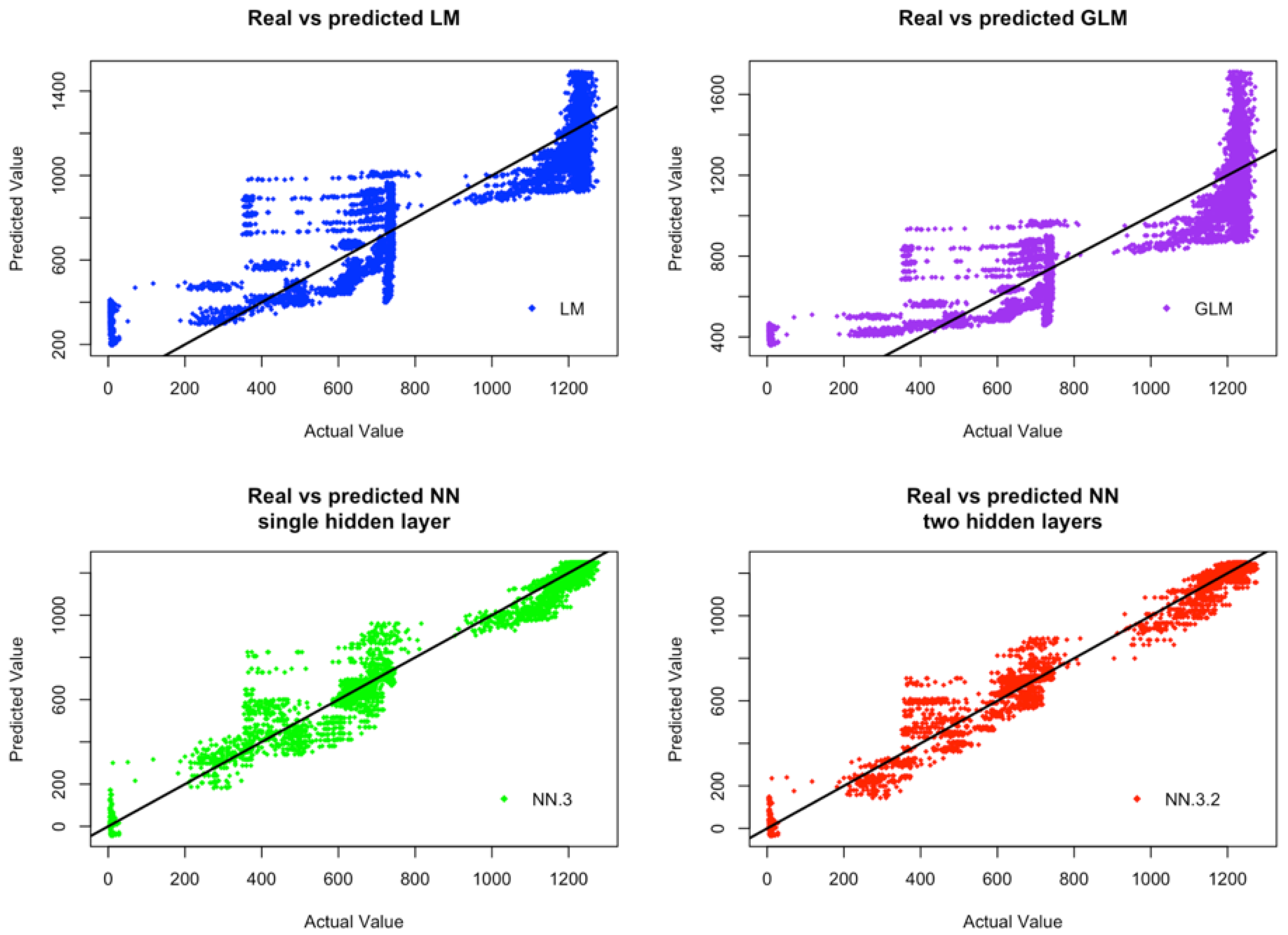
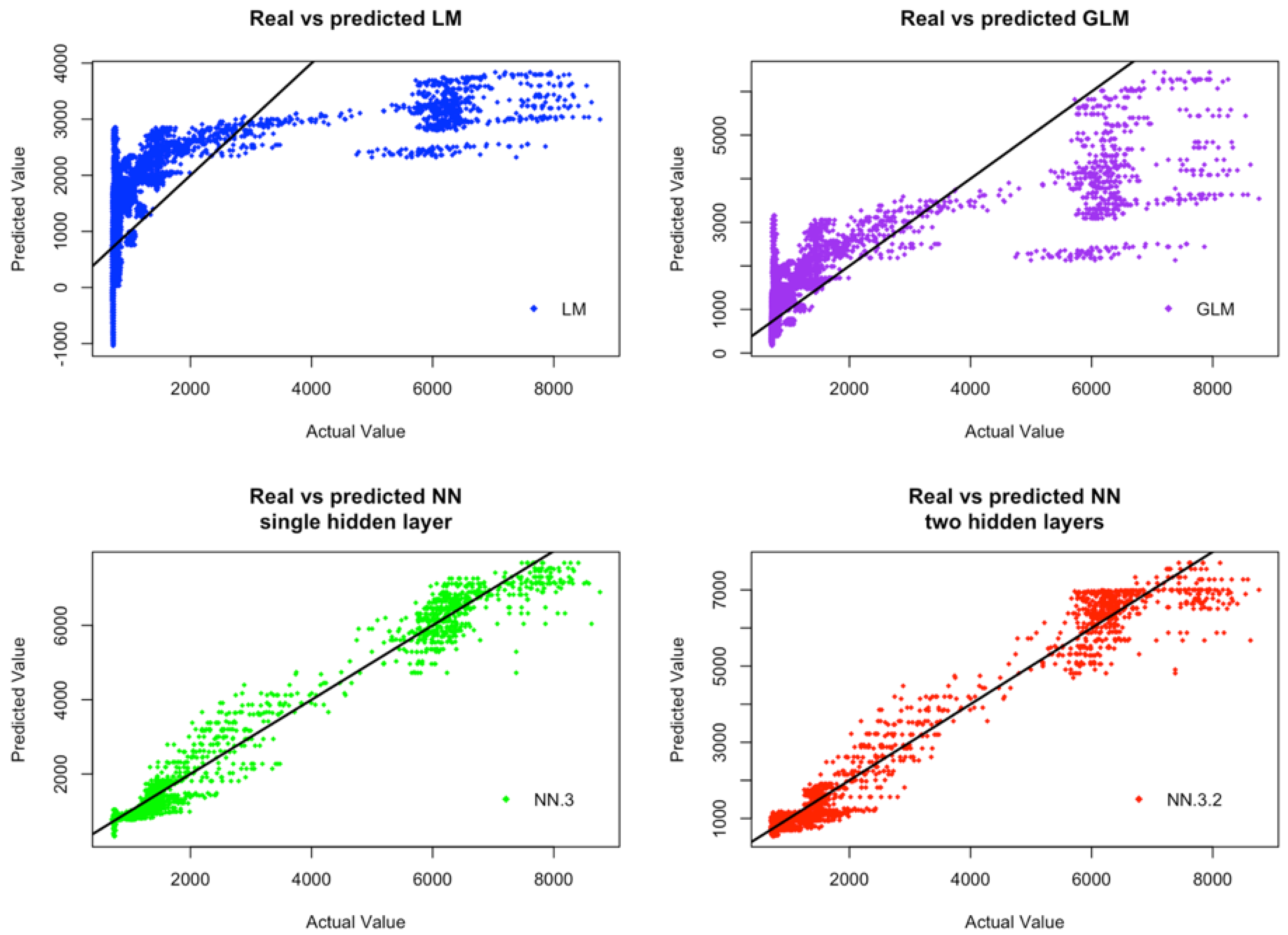
Figure 4 and
Figure 5 display respectively, for CCDs and IWDs, the plots of actual values against predicted values of the four considered models (i.e., LM, GLM, ANN-3, ANN-3-2). From these figures, we can observe that ANN models provide much more consistent results between the predicted values by these models and the actual observations. Furthermore, the overall variability of the predicted values by ANN models behaves more consistently than the variability of the predicted values by GLM and MLR models. Although, only the results associated with CCDs and IWDs are reported, the models performance is similar for ICDs and CWDs. Both GLM and MLR models fail to capture the functionality between the response variables and the input variables. These models fail, may be, because they are linear models and as such they are not able to capture the potential non-linear relationships between the input and output data. Furthermore, the model assumptions of GLM and MLR may be violated, because our simulation data are realizations of stochastic processes with unknown dependent structures.
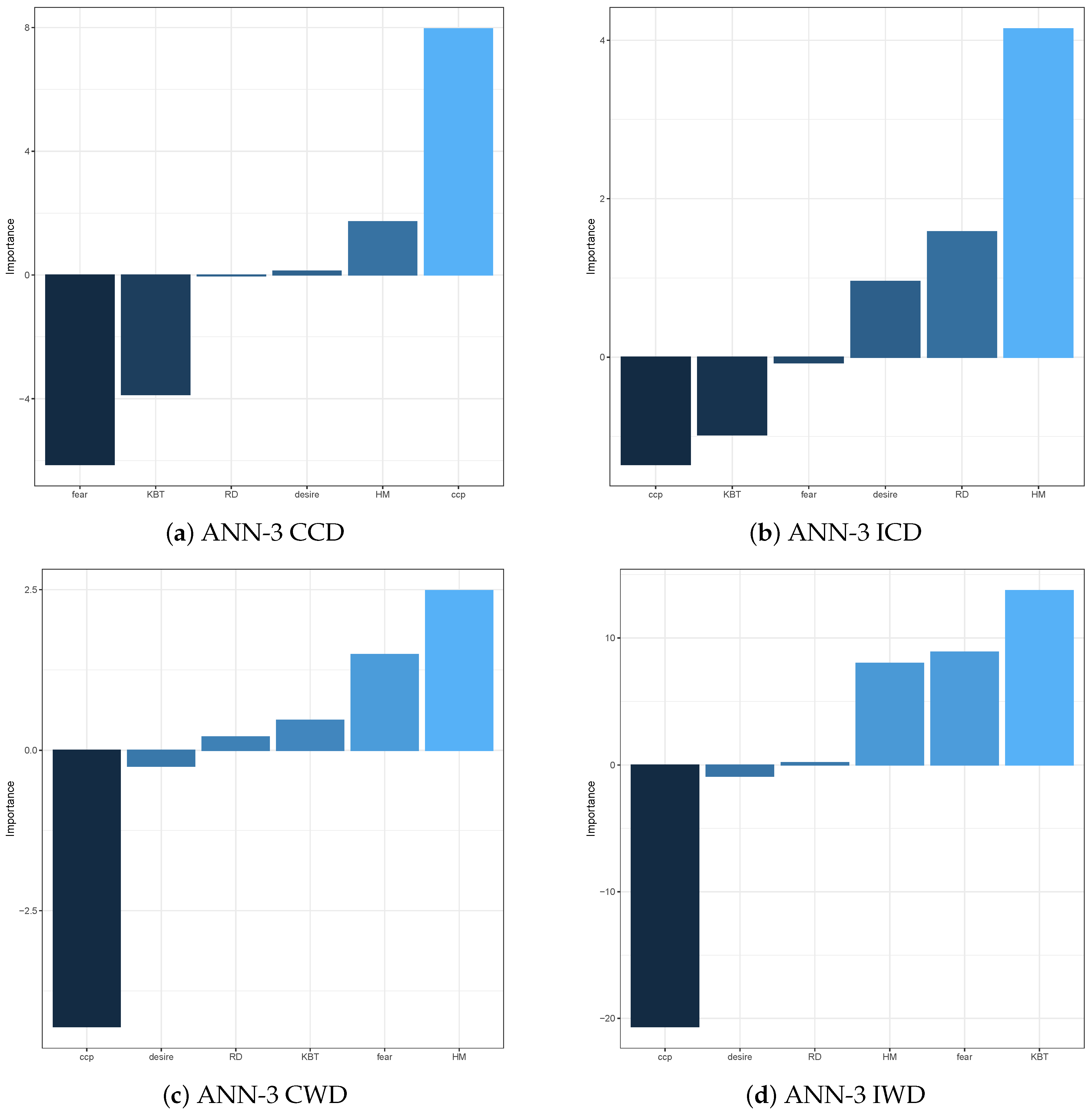
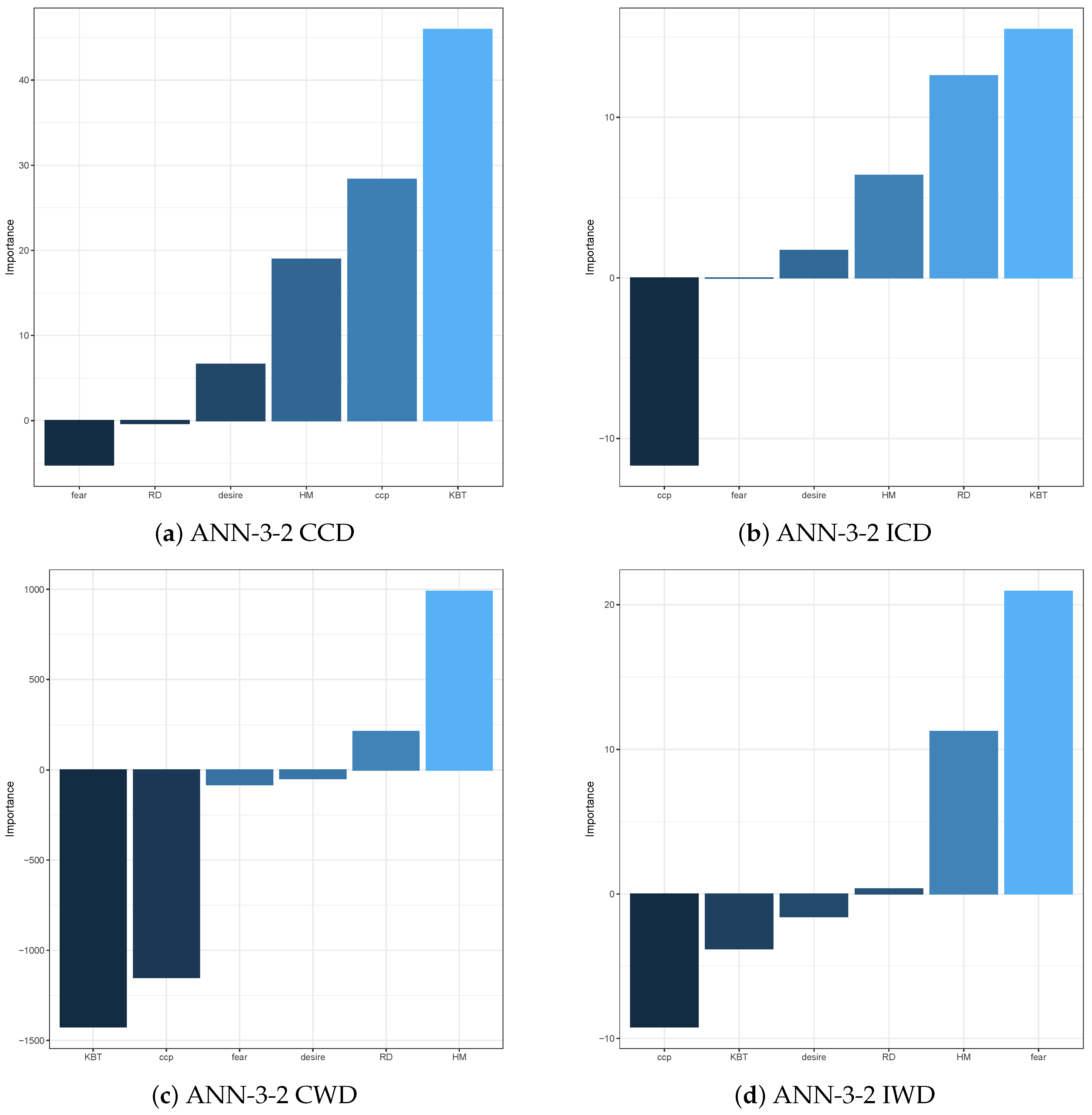
To help improve the explainability of ANN models in terms of variable importance, we compute the variable importance measures using Olden function, which is based on the obtained weights of the following layers connections: input-hidden, hidden-hidden, and hidden-output. These measures are displayed for ANN models, respectively, with output variables CCD, ICD, CWD and IWD in
Figure 6 and
Figure 7. In
Figure 6 these measures are displayed for ANN model with one hidden layer with three neurons, i.e., ANN-3. In
Figure 7 they are displayed for the ANN model with two hidden layers, with three neurons in the first hidden layer and two neurons in the second hidden layer, i.e., ANN-3-2. Overall, for both types of the ANN models and all types of input decisions, CCP is deemed to be the most crucial variable in explaining the variation of the response variables. The KBT seems to be the second most dominant factor to influence the crossing or waiting decisions, but the effect on these decisions is different. For the ANN model with multiple hidden layers, KBT appears to have a positive impact on the crossing decisions, while it has a negative effect on the waiting decisions. However, we observe a completely different phenomenon in the single hidden layer ANN model. This result may imply that, we cannot use the Olden function to determine the sign of the impact from the variables. We can only conclude their importance, but not the sign of their effect. More specifically, the factors CCP and KBT have a higher influence on the crossing decisions; in particular, KBT becomes the most influential on both CCD and ICD variables. In terms of waiting decisions, besides the influential factors CCP and KBT, common to both waiting decisions, HM is another crucial factor that affects the correct waiting decisions, while the most influential factor on the incorrect waiting decisions is Fear.
5. Discussions and Concluding Remarks
The traditional studies of complex systems have been mainly conducted through mathematical modelling via differential equations, application of dynamical systems and bifurcation theory to analyze the effects of the models’ parameters on the complex systems dynamics. With the development of mathematical models different from differential equations based, for example agent based simulation models, the traditional approaches of dynamical systems to understanding the effects of the models’ parameters on the complex systems dynamics often are not possible. Thus, to understand how parameters affect complex system dynamics and performance one must apply various statistical methods to the models’ simulation data. For example, one may try to apply various types of statistical modelling to the simulation data. From the statistical perspective, it is essential to investigate the simulation data through some modelling techniques, as they may provide better understanding of the behaviors of complex systems in engineering or other sciences. While the traditional linear or generalized linear models are working well for designed experiments of simple systems, they often do not perform well in the case of complex systems. Thus, more complex or non-linear models are required by the complex systems data, as such data may be non-linear and multi-scale, or may be obtained through some evolutionary computation.
In this work, we have conducted a statistical modelling study of simulation data of autonomous agents learning to cross CA-based highway model. We have investigated the modelling relationships between the input factors and output variables for our designed simulation experiments. We have proposed artificial neural network models as a regression technique for capturing the functionality between the input factors and response variables. Our study has demonstrated that the artificial neural network models outperform the classical statistical modelling approaches, including both multiple linear regression models and generalized linear models.
Due to the model assumptions associated with classical statistical models, both MLR and GLM have failed to explain the nature of our simulation data. In contrast, the ANN models have been more successful in establishing the mathematical relationships between input factors and output variables. Based on the results of the model validation, the ANN model with two hidden layers is the best model among other considered ones, in terms of model prediction accuracy and stability. Both linear and generalized linear models perform poorly in all cases considered, as they are linear models and one must make explicit model assumptions about the response variables. As a non-linear approach with the capability of performing adaptive model training, the ANN models provide more flexibility in building a model and they can be more successful in capturing the non-linear nature of the data. However, finding an optimal neural network for modelling simulation data may not be an easy task. Since the choice of the numbers of hidden layers or hidden neurons can be challenging, one must cross-validate all candidate models, to be able to determine the optimal one. A small number of hidden layers and hidden neurons can help to reduce the complexity of the models. Simple neural network models may be preferable from the complexity and computational point of view. However, they may fail to capture correctly some details of the relationships between input factors and output variables. By measuring the importance of the input factors using Olden function for different ANNs that are used to model the data corresponding to different decision types, we found that the most important factors affecting the decisions are CCP and KBT.
In the future, we plan to explore the optimal choices of the numbers of hidden layers and the numbers of hidden neurons, so that the model is optimal. It will also be interesting to compare the performance of ANNs with the deep learning approach to see if there is an improvement in explaining the model variation.


