Classification of Categorical Data Based on the Chi-Square Dissimilarity and t-SNE

Abstract

The recurrent use of databases with categorical variables in different applications demands new alternatives to identify relevant patterns. Classification is an interesting approach for the recognition of this type of data. However, there are a few amount of methods for this purpose in the literature. Also, those techniques are specifically focused only on kernels, having accuracy problems and high computational cost. For this reason, we propose an identification approach for categorical variables using conventional classifiers (LDC-QDC-KNN-SVM) and different mapping techniques to increase the separability of classes. Specifically, we map the initial features (categorical attributes) to another space, using the Chi-square (C-S) as a measure of dissimilarity. Then, we employ the (t-SNE) for reducing dimensionality of data to two or three features, allowing a significant reduction of computational times in learning methods. We evaluate the performance of proposed approach in terms of accuracy for several experimental configurations and public categorical datasets downloaded from the UCI repository, and we compare with relevant state of the art methods. Results show that C-S mapping and t-SNE considerably diminish the computational times in recognitions tasks, while the accuracy is preserved. Also, when we apply only the C-S mapping to the datasets, the separability of classes is enhanced, thus, the performance of learning algorithms is clearly increased.

1. Introduction

The high demand in the handling of all types of data, forces to companies, entities, and institutions to find underlying patterns. There are several ways to deal with this issue, in general, it is called data analysis [1]. A correct data processing requires basic knowledge in the type of databases, which can be nominal or quantitative. Nowadays, the algorithms and methodologies applied in data analysis focus on quantitative data, whether for clustering, regression and classification. In the literature, it can be seen a lot of proposed works related to this type of datasets such as spectral clustering [2], support vector machines (SMV) [3], Gaussian Processes (GP) [4], ordinary classification methods [5], among others. On the other hand, categorical data has not been widely studied. Therefore, there is a lack of sophisticated learning algorithms for this purpose. Currently, categorical data is mostly recognized with decision trees. However, this method has limitations due to low robustness and the performance is not satisfactory for validation data (low generalization capability). Categorical data have a particularity: high overlapping. For this reason, accuracy in automatic recognition is low. For labeling these data, an unsupervised method has been proposed: the Fuzzy C-means [6], but its computational time is high. Regarding this, some algorithms were introduced, such as coefficients of similarity [7], measures of dissimilarity [8], PAM [9], fuzzy statistics [10], dissimilarity measure for ranking data [11] and hierarchy of cluster [12].

An important alternative for solving the previously mentioned difficulties of qualitative databases, is the adaptation of the k-means to a dissimilarity space using the Chi-square (C-S) distance. It is a recently introduced algorithm for clustering ans its purpose is to map the categorical features through the C-S to another space with higher dimensionality, where the classes more separable. To the best of our knowledge, there are a several methodologies for clustering categorical datasets. However, we find a deficit in supervised schemes for classification. Although, some classifiers were applied to categorical variables [13,14,15], the data were not processed or mapped and the results obtained by these works were not satisfactory due to the complexity and overlapping of qualitative data (polls, tests, voting, among others). A positive fact, is that research works on explainable computational intelligence has gained much attention in many fields, including engineering, statistics, and natural and social science. Further, in machine learning, novel dimension reduction and feature extraction methods are particularly needed to facilitate data classification or clustering, depending on the availability of data labels [16].

In this work, we propose a methodology for performing classification of categorical datasets, based on the mapping of data to a real domain given by the Chi-square dissimilarity. The main goal is to augment the dimensionality of the feature space to increase the separability of classes. Additionally, this mapping allows to transform the integer input space ($\mathbf{X}\in {\mathbb{Z}}^D$) to a real space (${\mathbf{X}}^{*}\in {\mathbb{R}}^K$), making a more easier treatment for conventional classifiers. In our case, we apply the Bayesian linear classifier (LDC), Bayesian quadratic classifier (QDC), K-nearest neighbor (K-nn), and a support vector machine (SVM). The C-S mapping alleviate the overlapping in this type of data. Then, we employ the t-SNE to reduce dimensionality and computational times of learning algorithms decreases too [17].

An important aspect is that t-SNE preserves the data structure in a smaller input space (two or three dimensions). The t-SNE is one of the most used algorithms to perform dimensionality reduction to any database. It is worth noting that t-SNE is a parametric method, and it requires the setting of the number of neighbors, the perplexity hyper-parameter, and the distance metric. In our case, we implement the Chi-square distance, because the C-S is a suitable metric for categorical data [18].

We evaluate the performance of the proposed approach in terms of accuracy and computational times for several experimental configurations and public categorical datasets downloaded for the UCI repository: https://archive.ics.uci.edu/ml/index.php. Also, we compare our proposal with state of the art methods applied on five categorical databases: The sparse weighted naive Bayes classifier [14], coupled attribute similarity method [19], Boolean kernels [20], and a possibilistic naive Classifier with a generalized minimun-based algorithm [21]. Results show that C-S mapping and t-SNE considerably diminish the computational times in recognition tasks, while the accuracy is preserved in acceptable levels. Also, when we apply only the C-S mapping to the datasets, the separability of classes is enhanced, thus, the performance of learning algorithms is clearly increased. Outcomes indicates that the best identification is achieved when the categorical data is mapped with the C-S without reducing the input space using the t-SNE.

The rest of the paper is organized as follows: First, we describe the state of the art, next we detail the materials and methods. Then, we illustrate the results and discuss them. Finally, we give the conclusions of the proposed work.

2. State of the Art

The increasing use of datasets conformed by qualitative samples, demands new approaches to perform clustering. A first attempt was presented in [22], where categorical data is clustered with K-means. Specifically, the methodology transforms multiple categorical attributes in binary marks (1 for presence and 0 for the absence of a category). Next, these binary attributes are considered as numeric descriptors in the ordinary K-means algorithm. Nonetheless, this proposal requires to handle a great amount of binary points when the datasets have samples with many categories, which increases its computational cost and memory storage. Other proposed methods such as the similarity coefficient of Gower [7], dissimilarity measures [8], the PAM algorithm [9], hierarchy of cluster [12], statistic fuzzy algorithms [23] and conceptual clustering methods [10] have been reported. All of them have limited performance when are they are applied to massive data of type categorical.

Also, there are reports related to clustering analysis [9,24,25], where it is discussed issues regarding apply clustering methods over categorical data. However, none of these works give a feasible solution to the existing problems in non-numeric repositories. The main recommendation is to binarize the data and to use binary similarity measures, but the memory storage becomes the main difficulty. The authors of [26] implemented a study about distances for heterogeneous data (datasets with mixed qualitative and quantitative variables) based on a supervised framework, being each sample complemented with the respective class label. But, it is not generalizable to non-labeled databases. Recently, the authors of [27] developed a clustering algorithm which maps a categorical dataset into a Euclidean space. This method reveals the data configuration with a structure based clustering (SBC) scheme, achieving acceptable results in a positive identification of groups and classes, even improving the performance obtained by benchmark approaches for unsupervised learning: K-modes [28], dissimilarity distance [29], Mkm-nof and Mkm-ndm [30]. There are two considerable handicaps with the SBC framework: first, the high computational cost; secondly, the reduced accuracy for high dimensional datasets.

Many researchers developed various machine learning algorithms, i.e., GA and Fuzzy inference [31] artificial neural networks (ANN) [32], self-adaptive method [33], support vector machines (SVM) [34], Learning Vector Quantization (LVQ) [35], extreme learning machine [36], adaptive stochastic resonance [37], model-based class discrimination (VPMCD) [38], random forest [39], Artificial Bee Colony (ABC) [40], deep belief network [41], among others. All the aforementioned techniques are pretty complicated to interpret categorical data [42]. This is because of the reduction of the number of features (attributes) is a difficult task [43]. Theoretically, the presence of many features offers the opportunity to implement classifiers having better discriminating power. Nevertheless, this is not always true in practice, because not all features are relevant for representing the underlying phenomena of interest. Thus, when reducing the number of attributes, or when creating new ones, it is possible to achieve some benefits: Lower complexity of the classifier, reducing over-fitting, increasing the interpretability of the results, robustness to noise, and improving the accuracy of a basic classifier [44,45]. Most of dimensionality reduction models are developed for continuous data. This led to the search of dissimilarity measures to map the categorical data to a continuous domain [46]. An example of this is the dissimilarity measure based on the Chi-Square distance, that allows to map from a discrete space to a continuous one.

Related to supervised learning, several researchers proposed interesting frameworks. For example, in [14] was introduced an approach based on sparse weighted naive Bayes classifier [14], this work was the first attempt to extend sparse regression for processing categorical variables with competitive outcomes. Also, the authors of [19] developed a couple attribute similarity scheme to capture a global picture of the features. Furthermore, in [20] was presented a method composed of boolean kernels, here the basic concept is to create human-readable features to ease the extraction of interpretation rules directly from the embedding space. Finally, the research of [21] showed a classifier based on a naive possibilistic estimation with a generalized minimun-based algorithm. These relevant works, demonstrated that supervised algorithms can be adapted to categorical or qualitative data.

3. Materials and Methods

3.1. Chi-Square Distance

The chi-square distance is similar to the Euclidean. However, it is a weighted distance and a suitable metric for the analysis of databases with qualitative, categorical or nominal variables. The Chi-square distance compares the counts of responses from categorical variables with two or more independent features:

$$d_{ij}=\sqrt{\sum _{n=1}^D\frac{1}{{\tilde{x}}_n}{(\widetilde{x_{in}}-\widetilde{x_{jn}})}^2}$$

where

$${\displaystyle {\tilde{x}}_{in}=\frac{x_{in}}{{\displaystyle \sum _{n=1}^D{x}_{in}}}}$$

$${\tilde{x}}_n=\frac{1}{D}\sum _{n=1}^D{x}_{in}$$

Here, D is the number of features or dimensions. The Chi-square distance uses a contingency table, with the frequency of each attribute. The weighted distance C-S with categorical features allows a better treatment of these data. This is explained because it improves the separability of the classes, and allows an easier grouping or discrimination. However, an important drawback is the augment of dimensionality due to the data mapping to a space of dissimilarity. Therefore, it is necessary to use the algorithm t-SNE for reducing the dimensionality to 2 or 3 attributes. To preserve the structure of the databases, it was implemented the C-S metric within the distance function of t-SNE for simultaneously enhancing separability of categorical data and reducing computational times in learning algorithms [46].

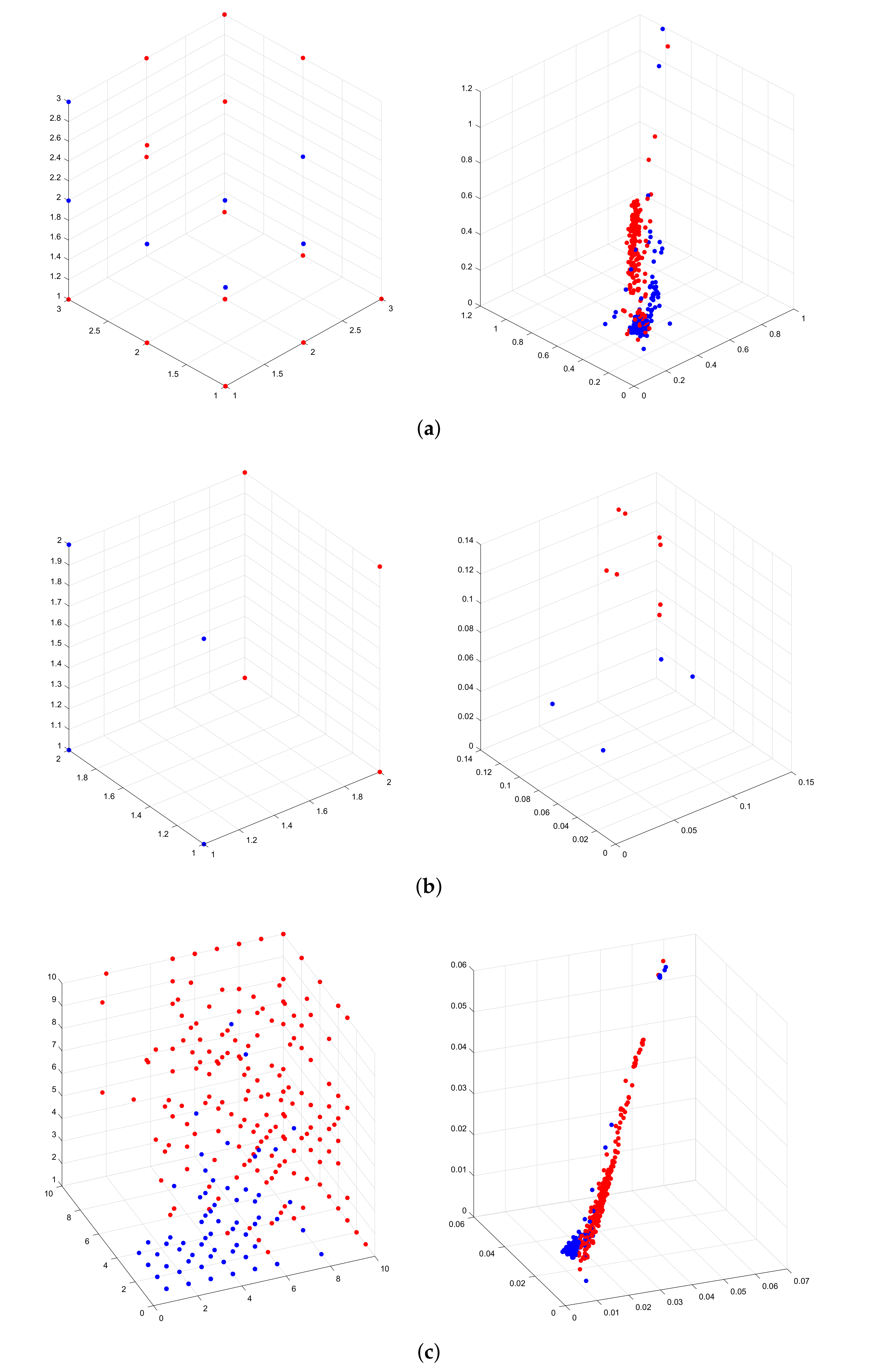
3.2. T-Distributed Stochastic Neighbor Embedding

t-distributed stochastic neighbor embedding (t-SNE) minimizes the divergence between two distributions: a distribution that measures similarities by pairs of input objects $\mathbf{X}=({\mathbf{x}}_1,{\mathbf{x}}_2,\dots ,{\mathbf{x}}_N)$∈${\mathbb{R}}^{D_1}$ and a distribution that measures similarities by pairs of the corresponding points of low dimension in the embedding $\mathbf{Y}=({\mathbf{y}}_1,{\mathbf{y}}_2,\dots ,{\mathbf{y}}_N)$∈${\mathbb{R}}^{D_2}$, being $D_1>D_2$. Suppose a dataset of N input objects $\mathbf{X}=({\mathbf{x}}_1,{\mathbf{x}}_2,\dots ,{\mathbf{x}}_N)$ and a function $d({\mathbf{x}}_i,{\mathbf{x}}_j)$ that calculates a distance between a pair of objects, for example, the Euclidean distance $d({\mathbf{x}}_i,{\mathbf{x}}_j)=\left|\right|{\mathbf{x}}_i-{\mathbf{x}}_j{\left|\right|}_2$. Then, t-SNE defines joint probabilities $p_{i,j}$ that measure the similarity between ${\mathbf{x}}_i$ and ${\mathbf{x}}_j$ [17]:

$$\begin{array}{cc}\hfill & p_{j|i}=\frac{exp(-d{({\mathbf{x}}_i,{\mathbf{x}}_j)}^2/2{\sigma }_i^2)}{{\sum }_{k\ne i}exp(-d{({\mathbf{x}}_i,{\mathbf{x}}_k)}^2)/2{\sigma }_i^2)},\hfill \\ \hfill & p_{i|i}=0\hfill \\ \hfill & \sum _{i,j}{P}_{i,j}=1\hfill \end{array}$$

Also:

$$p_{i,j}=p_{j,i}=\frac{p_{j|i}+p_{i|j}}{2N}$$

In the above formulation, the bandwidth of the Gaussian cores, ${\sigma }_i$, is set in such a way that the perplexity of the conditional distribution $p_i$ is equal to a predefined perplexity $\mu$. As a result, the optimal value of ${\sigma }_i$ varies depending on the object: in regions of the data space with a higher data density, ${\sigma }_i$ tends to be smaller, and vice versa. The optimal value of ${\sigma }_i$ for each input object can be found using a simple binary search [47] or a robust root search method.

The objective of t-SNE is to find a $D_2$-dimensional map $\mathbf{Y}=({\mathbf{y}}_1,{\mathbf{y}}_2,\dots ,{\mathbf{y}}_N)$∈${\mathbb{R}}^{D_2}$ for an optimal reflecting of the similarities $p_{i,j}$. Therefore, it measures the similarities $q_{i,j}$ between two points ${\mathbf{y}}_i$ y ${\mathbf{y}}_j$ in a similar way:

$$\begin{array}{cc}\hfill & q_{ji}=\frac{(1+||{\mathbf{y}}_i-{\mathbf{y}}_j{\left|\right|}^2{)}^{-1}}{{\sum }_k{\sum }_{k\ne l}(1+(\left|\right|{\mathbf{y}}_k-{\mathbf{y}}_l{\parallel \left|\right)}^2{)}^{-1}}\hfill \\ \hfill & q_{ii}=0\hfill \end{array}$$

The heavy tails of the normalized Student-t allow the modeling of dissimilar input objects ${\mathbf{x}}_i$ y ${\mathbf{x}}_j$ by low-dimensional counterparts ${\mathbf{y}}_i$ and ${\mathbf{y}}_j$. The locations of the insertion points ${\mathbf{y}}_i$ are determined by minimizing the divergence of Kullback-Leibler between the joint distributions P and Q:

$$C\left(\epsilon \right)=KL\left(P\right|\left|Q\right)=\sum _{i\ne j}{p}_{i,j}log\frac{p_{i,j}}{q_{i,j}}$$

Due to the asymmetry of the Kullback-Leibler divergence, the objective function focuses on modeling high values of $p_{ij}$ (similar objects) by high values of $q_{ij}$ (nearby points in the embedding space). The objective function is usually minimized when descending along the gradient [48]:

$$\frac{\partial C}{\partial {\mathbf{y}}_i}=4\sum _{j\ne i}(p_{ij}-q_{ij})q_{ij}z({\mathbf{y}}_i-{\mathbf{y}}_j)$$

3.3. Standard Classification Techniques

We test four standard classifiers at the supervised learning stage: Linear Bayesian (LDC), Quadratic Bayesian (QDC), Support Vector machine (SVM) and K-nn. The purpose is to demonstrate that the core of this work is the processing of categorical data through the Chi-square mapping for increasing class separability and t-SNE for dimensionality reduction.

3.3.1. Support Vector Machines (SVMs)

Support vector machines (SVMs) are prevalent in applications such as natural language processing, speech, image recognition and artificial vision. The full theory of SVMs can be found in [49]. This approach can be divided as follows:

• Separation of classes: It is about finding the optimal separating hyperplane between the two classes by maximizing the margin between the closest points of the classes.
• Overlapping classes: The incorrect data points of the discriminating margin are weighted to reduce their influence (soft margin).
• Non-linearity: When a linear separator cannot be found, the points are mapped to another dimensional space where the data can be separated linearly (this projection is realized via kernel techniques).
• Solution of the problem: The whole task can be formulated as a quadratic optimization problem that can be solved by known methods.

SVMs belong to a class of machine learning algorithms called kernel methods. Common kernels used in SVMs include: RBG or Gaussian, linear, polynomial, sigmoidal, among others [50]. We choose the RBG function due to its flexibility for different type of data. We set the Gamma and C hyper-parameters of the RBF kernel through cross-validation.

3.3.2. Bayesian Classifier

According to the Bayes rules, the probability of an example $E=(x_1,x_2,x_3,\dots ,x_D)$ be the class C is (where D is the number of attributes or features):

$$p\left(C\right|E)=\frac{p\left(E\right|C\left)p\right(C)}{p\left(E\right)},$$

E is classified as class $C=+$ if and only if:

$$f_b\left(E\right)=\frac{p(C=+|E)}{p(C=-|E)}\ge 1,$$

where $f_b\left(E\right)$ is called Bayesian classifier. Suppose that all attributes are independent of the class variable; that is to say,

$$P\left(E\right|C)=p(x_1,x_2,x_3,\dots ,x_D|C)=\prod _{i=1}^{D}p\left(x_i\right|C),$$

the resulting classifier is then:

$$f_b\left(E\right)=\frac{p(C=+)}{p(C=-)}\prod _{i=1}^N\frac{p\left(x_i\right|C=+)}{p\left(x_i\right|C=-)}.$$

The function $f_b\left(E\right)$ is called the Naive Bayes Classifier. The difference of the linear discriminant classifier (LDC) and quadratic (QDC) is the assumption of the covariance function. Specifically, if the covariance is assumed as equal for all classes, we refer to LDC, allowing a considerable mathematical simplicity for calculating the prediction distribution, but there is a possible loss of generalization capability. If the covariance is assumed different for all classes, we refer to QDC, and we can separate non-linear data with more accuracy, but the calculation of prediction distribution is more complex [51].

3.3.3. K-Nearest Neighbor (K-nn)

The learning process of the K-nn method is based on the storage of data. The method is described as follows:

• The training data $\mathbf{X}={\mathbf{x}}_1,{\mathbf{x}}_2,\dots ,{\mathbf{x}}_N$ with labels $\mathbf{y}=y_1,y_2,\dots ,y_N$ (being N the number of data samples) are stored in memory.
• For a new sample ${\mathbf{x}}_i$∈${\mathbb{R}}^D$, where D is the number of attributes, it is found the k-nearest neighbors using a distance d in the whole training set (k can be $1,3,5,7,\dots$).
• It is performed a voting procedure for selecting the class of the new sample ${\mathbf{x}}_i$.
• Common distances d are:

  -

  Mahalanobis:

  $$D_M(\mathbf{x},\mathbf{y})=\sqrt{{(\mathbf{x}-\mathbf{y})}^{\top }{\Sigma }^{-1}(\mathbf{x}-\mathbf{y})},$$

  where ${\Sigma }^{-1}$ is the covariance matrix between $\mathbf{x}$ and $\mathbf{y}$.

  -

  Euclidean:

  $$\left|\right|\mathbf{x}-{\mathbf{y}\left|\right|}_2=\sqrt{{(\mathbf{x}-\mathbf{y})}^{\top }(\mathbf{x}-\mathbf{y})}$$

  -

  Manhattan:

  $${Manh(\mathbf{x},\mathbf{y})=|(\mathbf{x}-\mathbf{y})}^{\top }(\mathbf{x}-\mathbf{y})|$$

  In this work, we employ the Mahalanobis distance. Also, we tested k = 3, 5, and 7 neighbors, but we report the best results obtained for k = 3.

4. Datasets and Experimental Setup

We test seven public datasets downloaded from UCI machine learning repository https://archive.ics.uci.edu/ml/index.php.

Table 1. Categorical datasets downloaded from public UCI repository.

Database	Samples	Features	Classes	Class Distribution
Audiology (Standardized) (A)	226	69	2	$\{124,76\}$
Balloons (B)	16	4	2	$\{12,8\}$
Breast Cancer (diagnosis) (BC)	699	9	2	$\{458,241\}$
Chess (King-Rook vs. King-Pawn) (C)	3196	36	2	$\{1669,1527\}$
Lymphography Domain (LD)	148	18	2	$\{81,61\}$
Molecular Biology (Promoter Gene Sequences) (MB)	106	57	2	$\{53,53\}$
Congressional Voting Records (V)	435	16	2	$\{267,168\}$

describes the databases and their main characteristics. First, we evaluate the t-SNE distances (Cosine, Jaccard, Mahalanobis, Chebychev, Minkowski, City block, Seuclidean, Euclidean, Chi-tsne) for demonstrating that C-S metric combined with the t-SNE algorithm (Chi-tsne), enhances separability of categorical databases. Then, we classify the datasets using four approaches (LDC, QDC, SVM, K-nn) to find which learning method is the most accurate in this context. For the sake of comparison, we test four different setups over the data: The single classifiers, the classifiers + t-SNE, the classifiers + C-S, and the classifiers + C-S + t-SNE). See

Table 2. Description of experimental setups

Experiment	Description
(A)	Database (A) + classifiers
(B)	Database (B) + classifiers
(BC)	Database (BC) + classifiers
(C)	Database (C) + classifiers
(LD)	Database (LD) + classifiers
(MB)	Database (MB) + classifiers
(V)	Database (V) + classifiers
(A) + (C-S)	Database (A) + Chi-Square Mapping + classifiers
(B) + (C-S)	Database (B) Chi-Square Mapping + classifiers
(BC) + (C-S)	Database (BC) + Chi-Square Mapping + classifiers
(C) + (C-S)	Database (C) + Chi-Square Mapping + classifiers
(LD) + (C-S)	Database (LD) + Chi-Square Mapping + classifiers
(MB) + (C-S)	Database (MB) + Chi-Square Mapping + classifiers
(V) + (C-S)	Database (V) + Chi-Square Mapping + classifiers
(A) + (C-S) + (t-SNE)	Database (A) + Chi-Square Mapping + t-SNE + classifiers
(B) + (C-S) + (t-SNE)	Database (B) + Chi-Square Mapping + t-SNE + classifiers
(BC) + (C-S) + (t-SNE)	Database (BC) + Chi-Square Mapping + t-SNE + classifiers
(C) + (C-S) + (t-SNE)	Database (C) + Chi-Square Mapping + t-SNE + classifiers
(LD) + (C-S) + (t-SNE)	Database (LD) + Chi-Square Mapping + t-SNE + classifiers
(MB) + (C-S) + (t-SNE)	Database (MB) + Chi-Square Mapping + t-SNE + classifiers
(V) + (C-S) + (t-SNE)	Database (V) + Chi-Square Mapping + t-SNE + classifiers
(A) + (t-SNE)	Database (A) + t-SNE + classifiers
(B) + (t-SNE)	Database (B) + t-SNE + classifiers
(BC) + (t-SNE)	Database (BC) + t-SNE + classifiers
(C) + (t-SNE)	Database (C) + t-SNE + classifiers
(LD) + (t-SNE)	Database (LD) + t-SNE + classifiers
(MB) + (t-SNE)	Database (MB) + t-SNE + classifiers
(V) + (t-SNE)	Database (V) + t-SNE + classifiers

for the description of the experimental setups. We calculate the accuracy (AC) and computational times for all classifiers in each setup, under the same conditions. We perform a hold-out validation scheme, with ten repetitions for each experiment, taking $70\%$ of the data for training and $30\%$ for validation. The simulations were performed with Matlab software on a server Intel (R) Xeon (R), CPU E5-2650 v2-2.60 GHz, two processors with eight cores, and 280 GB-RAM.

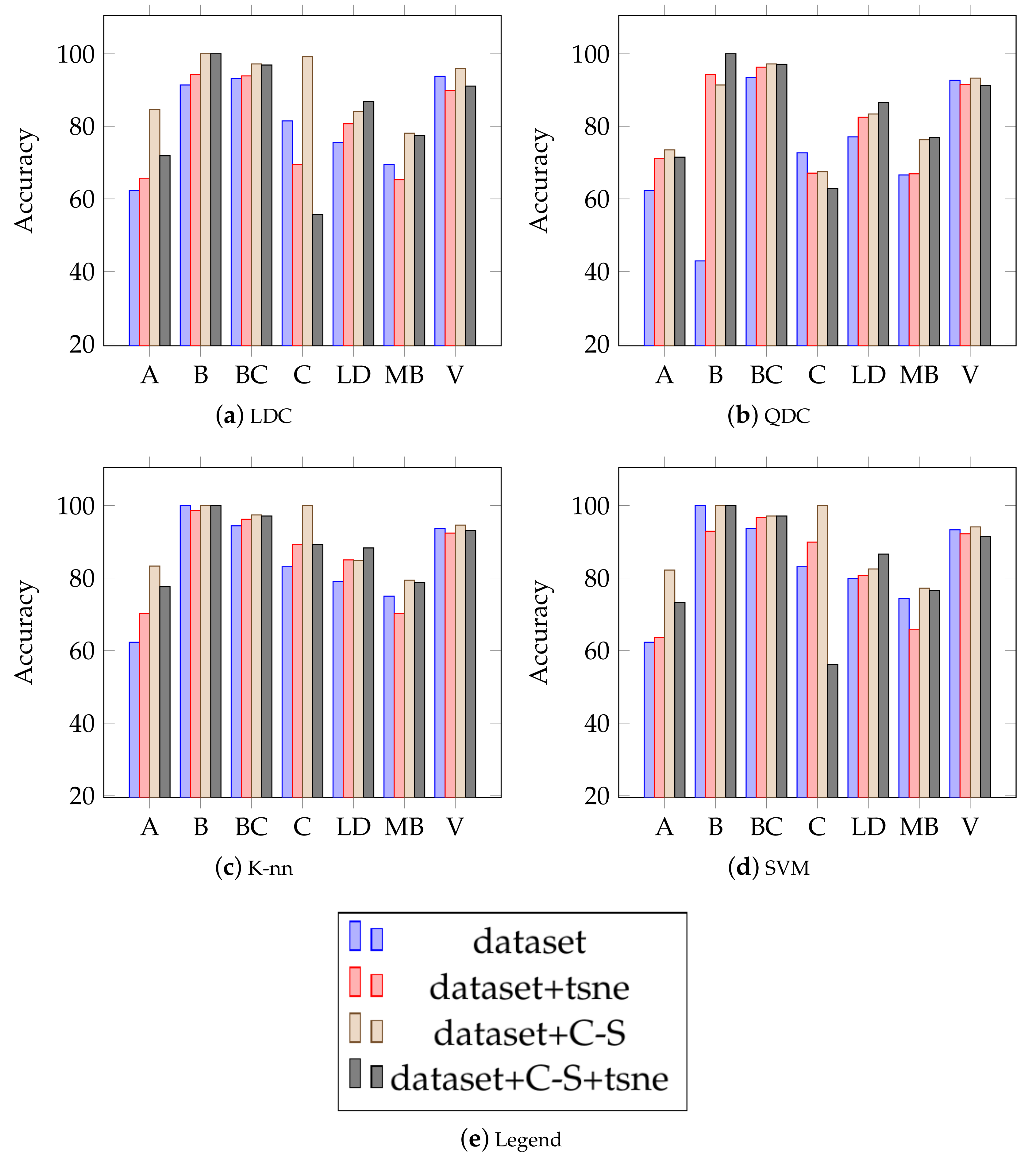
5. Results and Discussion

We observed from experimental results that the Chi-square (CS) distance is suitable for categorical data due to its mathematical nature. Initially, this divergence increases the dimension of data, maps the data to a real domain, and improves the separation of classes. Latter, we perform a dimension reduction with t-SNE for avoiding computational complexity. We do not consider another methods such as Kullback-Liebler divergence and Wasserstein distance, because they are especially developed for probabilistic distributions and estimation of parameters (KL is not symmetric, which can be an important limitation). However, this is not our case, because we do not assume a probability distribution over the categorical data. We pretend to map the categorical attributes to a real domain (instead of a integer domain) and increasing their separability.

According to the previously pointed out, the Figure 1 illustrates the main goal of the C-S. In this case, we show three of the seven databases (Congressional Voting Records, Balloons and Breast Cancer). We can see that original input space (left column) is highly overlapped and the features only take integers values. On the contrary, when the datasets are mapped with the C-S, the separability of data is increased.

Table 3. Classification results (accuracy) for several distances of the t-SNE algorithm over seven UCI public datasets. LDC and QDC correspond to linear and quadratic Bayesian classifier, K-nn stands for K-nearest neighbor and SVM is the support vector machine. The datasets: A, B, BC, C, LD, MB, V are defined in Table 1.

Dataset (A)	cosine	jaccard	mahalanobis	chebychev	minkowski	cityblock	seuclidean	euclidean	(A) Chi
LDC	62.5 ± 0.0	70.3 ± 0.1	71.1 ± 0.1	60.0 ± 0.4	69.2 ± 0.0	62.8 ± 0.0	61.2 ± 0.0	66.4 ± 0.0	73.4 ± 0.1
QDC	72.8 ± 0.1	83.1 ± 0.0	70.7 ± 0.0	58.5 ± 0.1	73.6 ± 0.3	73.9 ± 0.0	55.6 ± 0.0	69.3 ± 0.0	84.6 ± 0.0
K-nn	82.8 ± 0.0	84.8 ± 0.1	77.2 ± 0.0	79.3 ± 0.1	84.4 ± 0.1	85.1 ± 0.0	63.9 ± 0.1	80.8 ± 0.0	88.9 ± 0.0
SVM	62.3 ± 0.0	70.8 ± 0.1	71.1 ± 0.0	62.3 ± 0.0	62.6 ± 0.0	60.3 ± 0.0	62.3 ± 0.0	64.3 ± 0.0	76.7 ± 0.1
Average	70.1	77.2	72.5	65.0	72.5	70.5	60.7	70.2	80.9
Dataset (B)	cosine	jaccard	mahalanobis	chebychev	minkowski	cityblock	seuclidean	euclidean	(A) Chi
LDC	74.3 ± 0.2	82.9 ± 0.1	75.7 ± 0.2	78.6 ± 0.2	72.9 ± 0.1	92.9 ± 0.1	54.3 ± 0.1	92.9 ± 0.1	97.1 ± 0.1
QDC	71.4 ± 0.2	74.3 ± 0.1	71.4 ± 0.1	75.7 ± 0.2	84.3 ± 0.1	84.3 ± 0.1	75.7 ± 0.2	81.4 ± 0.2	91.4 ± 0.0
K-nn	75.7 ± 0.1	85.7 ± 0.1	88.6 ± 0.1	78.6 ± 0.2	85.7 ± 0.1	94.3 ± 0.1	67.1 ± 0.1	95.7 ± 0.0	100 ± 0.0
SVM	72.9 ± 0.1	84.3 ± 0.1	85.7 ± 0.2	78.6 ± 0.2	70.0 ± 0.1	94.3 ± 0.1	58.6 ± 0.1	90.0 ± 0.1	97.1 ± 0.1
Average	73.6	81.8	80.4	77.9	78.2	91.5	63.9	90.0	96.4
Dataset (BC)	cosine	jaccard	mahalanobis	chebychev	minkowski	cityblock	seuclidean	euclidean	(A) Chi
LDC	88.3 ± 0.0	94.3 ± 0.0	78.3 ± 0.0	96.3 ± 0.0	95.6 ± 0.0	96.6 ± 0.0	96.5 ± 0.0	96.4 ± 0.0	96.9 ± 0.0
QDC	90.6 ± 0.0	93.4 ± 0.0	89.2 ± 0.0	96.8 ± 0.0	96.6 ± 0.0	97.3 ± 0.0	96.5 ± 0.0	96.4 ± 0.0	97.3 ± 0.0
K-nn	90.1 ± 0.0	95.3 ± 0.1	91.8 ± 0.0	96.6 ± 0.0	96.7 ± 0.0	97.5 ± 0.0	96.7 ± 0.0	97.1 ± 0.0	97.4 ± 0.0
SVM	88.1 ± 0.0	94.4 ± 0.0	79.1 ± 0.0	96.4 ± 0.0	95.5 ± 0.0	96.6 ± 0.0	96.5 ± 0.0	96.5 ± 0.0	97.2 ± 0.0
Average	89.3	94.4	84.6	96.5	96.1	95.7	96.5	96.6	97.2
Dataset (C)	cosine	jaccard	mahalanobis	chebychev	minkowski	cityblock	seuclidean	euclidean	(A) Chi
LDC	60.8 ± 0.0	59.7 ± 0.0	57.8 ± 0.0	50.3 ± 0.0	60.9 ± 0.0	55.3 ± 0.0	62.4 ± 0.0	60.8 ± 0.0	68.2 ± 0.0
QDC	65.4 ± 0.0	60.1 ± 0.0	58.9 ± 0.0	53.9 ± 0.0	62.1 ± 0.0	63.1 ± 0.0	64.1 ± 0.0	65.2 ± 0.0	65.5 ± 0.0
K-nn	88.5 ± 0.0	70.8 ± 0.0	84.3 ± 0.0	53.0 ± 0.0	89.4 ± 0.0	89.5 ± 0.0	85.9 ± 0.0	89.1 ± 0.0	89.7 ± 0.0
SVM	62.6 ± 0.0	60.7 ± 0.0	58.6 ± 0.0	52.2 ± 0.0	61.5 ± 0.0	60.8 ± 0.0	62.5 ± 0.0	61.1 ± 0.0	68.7 ± 0.0
Average	69.3	62.8	64.9	52.4	68.5	67.2	68.7	69.1	73.8
Dataset (LD)	cosine	jaccard	mahalanobis	chebychev	minkowski	cityblock	seuclidean	euclidean	(A) Chi
LDC	76.6 ± 0.0	71.6 ± 0.1	68.9 ± 0.1	64.3 ± 0.1	65.9 ± 0.1	76.1 ± 0.0	76.6 ± 0.0	72.0 ± 0.1	81.6 ± 0.1
QDC	77.3 ± 0.1	76.1 ± 0.0	64.1 ± 0.1	67.5 ± 0.1	67.0 ± 0.1	77.5 ± 0.0	78.6 ± 0.0	73.6 ± 0.1	81.1 ± 0.1
K-nn	79.1 ± 0.1	76.4 ± 0.1	79.1 ± 0.1	72.5 ± 0.1	74.8 ± 0.1	80.7 ± 0.0	83.4 ± 0.0	78.6 ± 0.1	84.0 ± 0.1
SVM	75.0 ± 0.0	71.1 ± 0.1	68.1 ± 0.1	66.1 ± 0.1	68.6 ± 0.1	75.9 ± 0.5	78.9 ± 0.0	70.7 ± 0.0	81.8 ± 0.1
Average	77.0	73.8	70.0	67.6	69.1	77.6	79.4	73.7	82.9
Dataset (MB)	cosine	jaccard	mahalanobis	chebychev	minkowski	cityblock	seuclidean	euclidean	(A) Chi
LDC	47.8 ± 0.1	56.2 ± 0.1	60.0 ± 0.1	43.1 ± 0.1	60.3 ± 0.1	72.5 ± 0.1	62.5 ± 0.1	55.0 ± 0.1	76.2 ± 0.1
QDC	57.2 ± 0.1	71.2 ± 0.1	54.1 ± 0.1	57.5 ± 0.1	68.7 ± 0.1	74.7 ± 0.1	65.3 ± 0.1	58.4 ± 0.1	78.7 ± 0.1
K-nn	62.5 ± 0.1	70.9 ± 0.1	65.6 ± 0.1	50.9 ± 0.1	66.2 ± 0.0	75.6 ± 0.1	68.1 ± 0.1	70.6 ± 0.1	80.3 ± 0.1
SVM	52.2 ± 0.1	55.9 ± 0.1	61.6 ± 0.1	44.4 ± 0.1	56.6 ± 0.1	70.3 ± 0.1	63.7 ± 0.1	54.1 ± 0.1	76.6 ± 0.1
Average	54.9	63.6	60.3	49.0	63.0	73.3	64.9	59.7	78.0
Dataset (V)	cosine	jaccard	mahalanobis	chebychev	minkowski	cityblock	seuclidean	euclidean	(A) Chi
LDC	90.5 ± 0.0	88.9 ± 0.0	90.0 ± 0.0	73.7 ± 0.0	90.2 ± 0.0	91.4 ± 0.0	80.8 ± 0.0	90.1 ± 0.0	91.5 ± 0.0
QDC	90.5 ± 0.0	90.9 ± 0.0	90.0 ± 0.0	74.5 ± 0.0	92.1 ± 0.0	91.7 ± 0.0	81.4 ± 0.0	90.6 ± 0.0	91.4 ± 0.0
K-nn	92.6 ± 0.0	91.7 ± 0.0	91.4 ± 0.0	76.6 ± 0.0	92.3 ± 0.0	93.3 ± 0.0	82.7 ± 0.0	92.3 ± 0.0	93.8 ± 0.0
SVM	91.4 ± 0.0	90.9 ± 0.0	89.8 ± 0.0	75.2 ± 0.0	91.9 ± 0.0	92.3 ± 0.0	81.7 ± 0.0	90.8 ± 0.0	92.6 ± 0.0
Average	91.2	90.6	90.4	75.0	91.6	92.2	81.6	90.9	93.1

shows the accuracy and standard deviation for LDC, QDC, SVM, and K-nn, when we use the t-SNE algorithm over the databases. The objective was to evaluate the distances (Cosine, Jaccard, Mahalanobis, Chebychev, Minkowski, City block, Seuclidean, Euclidean) commonly applied in t-SNE method and to demonstrate that C-S is the most suitable for categorical attributes. We can see that C-S metric outperforms the comparison distances with statistically significant differences in most of cases. Also, the t-SNE reduces the dimensionality of mapped data without a losing of relevant information or structure of data.

Figure 2 shows the accuracy achieved for each learning method in different experimental setups described in Table 2. We can identify four different setups for each dataset. The first one, consists of evaluating the standard classifiers in categorical databases without any processing or mapping the data. We can observe that classification outcomes are not the best for each dataset. This probes that categorical data must be processed or mapped before the recognition tasks.

In the second setup, we test the classifiers over the datasets mapped with the C-S dissimilarity. This allows to obtain a better separability, but a higher dimensionality which means major computational times. However, the C-S mapping generates the best classification results for all datasets, as we see in Figure 2. We consider this mapping transforms the categorical data to quantitative, and learning methods performs much better in this scenario. We explain this as follows: The primary function of the C-S mapping is to increase the dimensionality of data to alleviate he overlap of categorical features. Recall that categorical attributes are integers: $\mathbf{X}\in {\mathbb{Z}}^D$. When $\mathbf{X}$ is mapped with the C-S dissimilarity, the feature domain is transformed too, i.e $\mathbf{X}\in {\mathbb{Z}}^D\to {\mathbf{X}}^{*}\in {\mathbb{R}}^K$ with $K>D$. For this reason, the C-S mapping realizes a transformation from categorical to quantitative data.

In the third setup, we perform a combination of processing techniques. We initially map the data with the C-S dissimilarity. Then, we apply the Chi-tSNE algorithm for reducing the number of attributes to three. This reduction of dimensionality diminishes computational times while preserves the data structure. Accuracy results are comparable with the the first setup, but computational times are highly better than the other setups. This setup is the suitable for on-line recognitions systems.

Finally, the fourth setup applies the Chi-tSNE directly over the categorical datasets without a C-S mapping. Although, computational times demanded for training the learning algorithms are lower, the accuracy is affected.

In general, we can see in Figure 2 that the best setup in terms of accuracy was the second one, when the categorical features (integer values) are mapped with the C-S dissimilarity to a real space (quantitative) with higher dimensionality, achieving a better separability. It should be noted that the best classifier was the K-nn in most of experiments. It is important to mention that the most efficient method in computational cost was in the third setup as shown in

Table 4. Computational times for standard classifiers tested in seven UCI public datasets. The datasets: A, B, BC, C, LD, MB, V are described in Table 1.

Experimental Setup	Computational Time (Seconds)	Experimental Setup t-SNE	Computational Time (Seconds)
(A) + C-S	33.8	(A) + C-S + t-SNE	24.6
(B) + C-S	1.4	(B) + C-S + t-SNE	0.2
(BC) + C-S	397.0	(BC) + C-S + t-SNE	86.0
(C) + C-S	30.9	(C) + C-S + t-SNE	21.5
(LD) + C-S	25.9	(LD) + C-S + t-SNE	18.3
(MB) + C-S	155.4	(MB) + C-S + t-SNE	52.6
(V) + C-S	2530.5	(V) + C-S + t-SNE	523.5

. This is remarkable, because the percentages of accuracy are competitive, with the addition of achieving the lowest computational times.

Finally, to demonstrate the efficiency of our method, we made a comparison with several classification methods reported in the literature for recognition of categorical databases: the sparse weighted naive Bayes classifier [14], coupled attribute similarity method [19], Boolean kernels [20], and a possibilistic naive Classifier with a generalized minimun-based algorithm [21]. We find five databases of the seven that we use in this paper. We obtain better classification accuracy with our proposed methodology than comparison methods, as can be seen in

Table 5. Accuracy results in identification of categorical data for the comparison methods versus the C-S approach. SWNBC corresponds to the sparse weighted naive Bayes classifier [14], C4.5 is the coupled attribute similarity method [19], BK is the classifier based on Boolean kernel [20], and NPC is the naive possibilistic classifier [21].

Database	SWNBC	C4.5	BK	NPC	C-S
Chess	87.59 ± 1.23	97.48 ± 1.85	97.22 ± 1.94	88.67 ± 1.72	100.0 ± 0.00
Congressional Voting	90.08 ± 3.71	93.28 ± 3.18	92.36 ± 3.23	94.23 ± 3.62	94.53 ± 1.60
Breast Cancer	72.50 ± 7.71	71.33 ± 6.33	66.45 ± 6.92	73.81 ± 7.11	97.35 ± 1.30
Lymphography Domain	83.60 ± 9.82	73.12 ± 8.63	73.82 ± 8.47	87.76 ± 9.60	88.30 ± 4.80
Balloons	100.0 ± 0.00	100.0 ± 0.00	100.0 ± 0.00	100.0 ± 0.00	100.0 ± 0.00

.

6. Conclusions and Future Work

In this work, we implemented a recognition approach for categorical data. To do this, we developed two interesting and suitable options. First, we mapped the categorical attributes to a higher dimensionality space with a Chi-square (C-S) dissimilarity. This procedure allows to transform the feature domain of categorical datasets from integers to real values, alleviating the overlapping problem. We can observe from Figure 1 that a mapping of categorical data increases recognition accuracy. Second, we introduced an alternative distance based on Chi-square in the t-stochastic neighbor embedding method (tSNE), see Table 3 for results. The combination of the C-S dissimilarity and the Chi-tSNE applied on categorical data, simultaneously increases data separability and reduces the computational times for classification, when we tested standard classifiers: LDC, QDC, k-nn and SVM over public categorical datasets downloaded from the UCI repository, as we showed in Table 4. Also, we described how our proposal using C-S as a measure of dissimilarity outperformed other methods for classification of categorical data reported in the literature [14,19,20,21], see Table 5.

As future work, we propose a new metric based on a kernel formulation specially designed for qualitative databases, for example Boolean kernels. Also we would like to evaluate advanced classifiers such as Gaussian processes or deep learning. Finally, we encourage the reader to perform an analysis of the Chi-square and its invariance properties based on Wasserstein Information Matrix [52].

References

1. Janert, P.K. Data Analysis with Open Source Tools: A Hands-On Guide for Programmers and Data Scientists; O’Reilly Media, Inc.: Newton, MA, USA, 2010. [Google Scholar]
2. Ng, A.Y.; Jordan, M.I.; Weiss, Y. On spectral clustering: Analysis and an algorithm. In Advances in Neural Information Processing Systems; MIT Press: Cambridge, MA, USA, 2002; pp. 849–856. [Google Scholar]
3. Meyer, D.; Wien, F.T. Support vector machines. R News 2001, 1, 23–26. [Google Scholar]
4. Rasmussen, C.E. Gaussian processes in machine learning. In Advanced Lectures on Machine Learning; Springer: Berlin/Heidelberg, Germany, 2004; pp. 63–71. [Google Scholar]
5. Wang, Y.; Zhu, L. Research on improved text classification method based on combined weighted model. Concurr. Comput. Pract. Exp. 2020, 32, e5140. [Google Scholar] [CrossRef]
6. Huang, Z.; Ng, M.K. A fuzzy k-modes algorithm for clustering categorical data. IEEE Trans. Fuzzy Syst. 1999, 7, 446–452. [Google Scholar] [CrossRef] [Green Version]
7. Gower, J.C. A general coefficient of similarity and some of its properties. Biometrics 1971, 27, 857–871. [Google Scholar] [CrossRef]
8. Gowda, K. Symbolic clustering using a new dissimilarity measure. Pattern Recognit. 1991, 24, 567–578. [Google Scholar] [CrossRef]
9. Kaufman, L. Finding Groups in Data: An Introduction to Cluster Analysis; John Wiley and Sons: Hoboken, NJ, USA, 2009; Volume 344. [Google Scholar]
10. Michalski, R.S. Automated construction of classifications: Conceptual clustering versus numerical taxonomy. IEEE Trans. Pattern Anal. Mach. Intell. 1983, 4, 396–410. [Google Scholar] [CrossRef]
11. Bonanomi, A.; Nai Ruscone, M.; Osmetti, S.A. Dissimilarity measure for ranking data via mixture of copulae. Stat. Anal. Data Min. ASA Data Sci. J. 2019, 12, 412–425. [Google Scholar] [CrossRef]
12. Seshadri, K.; Iyer, K.V. Design and evaluation of a parallel document clustering algorithm based on hierarchical latent semantic analysis. Concurr. Comput. Pract. Exp. 2019, 31, e5094. [Google Scholar] [CrossRef]
13. Alexandridis, A.; Chondrodima, E.; Giannopoulos, N.; Sarimveis, H. A fast and efficient method for training categorical radial basis function networks. IEEE Trans. Neural Netw. Learn. Syst. 2017, 28, 2831–2836. [Google Scholar] [CrossRef]
14. Zheng, Z.; Cai, Y.; Yang, Y.; Li, Y. Sparse Weighted Naive Bayes Classifier for Efficient Classification of Categorical Data. In Proceedings of the 2018 IEEE Third International Conference on Data Science in Cyberspace (DSC), Guangzhou, China, 18–21 June 2018; IEEE: Piscataway, NJ, USA, 2018; pp. 691–696. [Google Scholar]
15. Villuendas-Rey, Y.; Rey-Benguría, C.F.; Ferreira-Santiago, Á.; Camacho-Nieto, O.; Yáñez-Márquez, C. The naïve associative classifier (NAC): A novel, simple, transparent, and accurate classification model evaluated on financial data. Neurocomputing 2017, 265, 105–115. [Google Scholar] [CrossRef]
16. Computation, Special Issue “Explainable Computational Intelligence, Theory, Methods and Applications”. 2020. Available online: https://0-www-mdpi-com.brum.beds.ac.uk/journal/computation/special_issues/explainable_computational_intelligence (accessed on 5 September 2020).
17. Maaten, L.V.D.; Hinton, G. Visualizing data using t-SNE. J. Mach. Learn. Res. 2008, 9, 2579–2605. [Google Scholar]
18. Field, A. Discovering Statistics Using IBM SPSS Statistics; Sage: Newcastle upon Tyne, UK, 2013. [Google Scholar]
19. Wang, C.; Dong, X.; Zhou, F.; Cao, L.; Chi, C.H. Coupled attribute similarity learning on categorical data. IEEE Trans. Neural Netw. Learn. Syst. 2015, 26, 781–797. [Google Scholar] [CrossRef] [PubMed]
20. Polato, M.; Lauriola, I.; Aiolli, F. A novel boolean kernels family for categorical data. Entropy 2018, 20, 444. [Google Scholar] [CrossRef] [Green Version]
21. Baati, K.; Hamdani, T.M.; Alimi, A.M.; Abraham, A. A new classifier for categorical data based on a possibilistic estimation and a novel generalized minimum-based algorithm. J. Intell. Fuzzy Syst. 2017, 33, 1723–1731. [Google Scholar] [CrossRef]
22. Ralambondrainy, H. A conceptual version of the k-means algorithm. Pattern Recognit. Lett. 1995, 16, 1147–1157. [Google Scholar] [CrossRef]
23. Max, A. Woodbury and Jonathan Clive. Clinical pure types as a fuzzy partition. J. Cybern. 1974, 4, 111–121. [Google Scholar]
24. Ahmad, A.; Dey, L. A method to compute distance between two categorical values of same attribute in unsupervised learning for categorical data set. Pattern Recognit. Lett. 2007, 28, 110–118. [Google Scholar] [CrossRef]
25. Jain, A.K.; Dubes, R.C. Algorithms for Clustering Data; Prentice-Hall, Inc.: Upper Saddle River, NJ, USA, 1988. [Google Scholar]
26. Wilson, D.R.; Martinez, T.R. Improved heterogeneous distance functions. J. Artif. Intell. Res. 1997, 6, 1–34. [Google Scholar] [CrossRef]
27. Qian, Y.; Li, F.; Liang, J.; Liu, B.; Dang, C. Space structure and clustering of categorical data. IEEE Trans. Neural Netw. Learn. Syst. 2016, 27, 2047–2059. [Google Scholar] [CrossRef]
28. Huang, Z. A fast clustering algorithm to cluster very large categorical data sets in data mining. DMKD 1997, 3, 34–39. [Google Scholar]
29. Chan, E.Y.; Ching, W.K.; Ng, M.K.; Huang, J.Z. An optimization algorithm for clustering using weighted dissimilarity measures. Pattern Recognit. 2004, 37, 943–952. [Google Scholar] [CrossRef]
30. Bai, L.; Liang, J.; Dang, C.; Cao, F. The impact of cluster representatives on the convergence of the k-modes type clustering. IEEE Trans. Pattern Anal. Mach. Intell. 2013, 35, 1509–1522. [Google Scholar] [CrossRef]
31. Kobayashi, Y.; Song, L.; Tomita, M.; Chen, P. Automatic Fault Detection and Isolation Method for Roller Bearing Using Hybrid-GA and Sequential Fuzzy Inference. Sensors 2019, 19, 3553. [Google Scholar] [CrossRef] [PubMed] [Green Version]
32. Ali, J.B.; Fnaiech, N.; Saidi, L.; Chebel-Morello, B.; Fnaiech, F. Application of empirical mode decomposition and artificial neural network for automatic bearing fault diagnosis based on vibration signals. Appl. Acoust. 2015, 89, 16–27. [Google Scholar]
33. Tian, Y.; Wang, Z.; Lu, C. Self-adaptive bearing fault diagnosis based on permutation entropy and manifold-based dynamic time warping. Mech. Syst. Signal Process. 2019, 114, 658–673. [Google Scholar] [CrossRef]
34. Tan, J.; Fu, W.; Wang, K.; Xue, X.; Hu, W.; Shan, Y. Fault Diagnosis for Rolling Bearing Based on Semi-Supervised Clustering and Support Vector Data Description with Adaptive Parameter Optimization and Improved Decision Strategy. Appl. Sci. 2019, 9, 1676. [Google Scholar] [CrossRef] [Green Version]
35. Kaden, M.; Lange, M.; Nebel, D.; Riedel, M.; Geweniger, T.; Villmann, T. Aspects in classification Learning—Review of recent developments in learning vector quantization. Found. Comput. Decis. Sci. 2014, 39, 79–105. [Google Scholar] [CrossRef] [Green Version]
36. Tian, Y.; Ma, J.; Lu, C.; Wang, Z. Rolling bearing fault diagnosis under variable conditions using LMD-SVD and extreme learning machine. Mech. Mach. Theory 2015, 90, 175–186. [Google Scholar] [CrossRef]
37. Zhou, P.; Lu, S.; Liu, F.; Liu, Y.; Li, G.; Zhao, J. Novel synthetic index-based adaptive stochastic resonance method and its application in bearing fault diagnosis. J. Sound Vib. 2017, 391, 194–210. [Google Scholar] [CrossRef]
38. Yang, Y.; Pan, H.; Ma, L.; Cheng, J. A fault diagnosis approach for roller bearing based on improved intrinsic timescale decomposition de-noising and kriging-variable predictive model-based class discriminate. J. Vib. Control 2016, 22, 1431–1446. [Google Scholar] [CrossRef]
39. Chen, Y.; Zhang, T.; Zhao, W.; Luo, Z.; Sun, K. Fault Diagnosis of Rolling Bearing Using Multiscale Amplitude-Aware Permutation Entropy and Random Forest. Algorithms 2019, 12, 184. [Google Scholar] [CrossRef] [Green Version]
40. Fei, S.W. Kurtosis forecasting of bearing vibration signal based on the hybrid model of empirical mode decomposition and RVM with artificial bee colony algorithm. Expert Syst. Appl. 2015, 42, 5011–5018. [Google Scholar] [CrossRef]
41. Shen, C.; Xie, J.; Wang, D.; Jiang, X.; Shi, J. Improved Hierarchical Adaptive Deep Belief Network for Bearing Fault Diagnosis. Appl. Sci. 2019, 9, 3374. [Google Scholar] [CrossRef] [Green Version]
42. Anbu, S.; Thangavelu, A.; Ashok, S.D. Fuzzy C-Means Based Clustering and Rule Formation Approach for Classification of Bearing Faults Using Discrete Wavelet Transform. Computation 2019, 7, 54. [Google Scholar] [CrossRef] [Green Version]
43. Cang, S.; Yu, H. Mutual information based input feature selection for classification problems. Decis. Support Syst. 2012, 54, 691–698. [Google Scholar] [CrossRef]
44. Sani, L.; Pecori, R.; Mordonini, M.; Cagnoni, S. From Complex System Analysis to Pattern Recognition: Experimental Assessment of an Unsupervised Feature Extraction Method Based on the Relevance Index Metrics. Computation 2019, 7, 39. [Google Scholar] [CrossRef] [Green Version]
45. Weber, M. Implications of PCCA+ in molecular simulation. Computation 2018, 6, 20. [Google Scholar] [CrossRef] [Green Version]
46. Serna, L.A.; Hernández, K.A.; González, P.N. A K-Means Clustering Algorithm: Using the Chi-Square as a Distance. In International Conference on Human Centered Computing; Tang, Y., Zu, Q., Rodríguez García, J., Eds.; Lecture Notes in Computer Science; Springer: Cham, Switzerland, 2019; Volume 11354. [Google Scholar]
47. Hinton, G.E.; Roweis, S.T. Stochastic neighbor embedding. In Advances in Neural Information Processing Systems; MIT Press: Cambridge, MA, USA, 2003; pp. 857–864. [Google Scholar]
48. Van Der Maaten, L. Accelerating t-SNE using tree-based algorithms. J. Mach. Learn. Res. 2014, 15, 3221–3245. [Google Scholar]
49. Cortes, C.; Vapnik, V. Support-vector network. Mach. Learn. 1995, 20, 1–25. [Google Scholar] [CrossRef]
50. Hu, M.; Chen, Y.; Kwok, J.T.Y. Building sparse multiple-kernel SVM classifiers. Learning (MKL) 2009, 3, 26. [Google Scholar]
51. Büyüköztürk, Ş.; Çokluk-Bökeoğlu, Ö. Discriminant function analysis: Concept and application. Eğitim Araştırmaları Dergisi 2008, 33, 73–92. [Google Scholar]
52. Li, W.; Zhao, J. Wasserstein information matrix. arXiv 2020, arXiv:1910.11248. [Google Scholar]
Figure 1. Initial categorical input space taking three attributes (left) and mapped features with Chi-tSNE (right) for: (a) Congressional Voting Records, (b) Balloons, and (c) Breast Cancer. Red and blue dots correspond to class 1 and 2, respectively. Each dimension of subfigures is a random feature.
Computation 08 00104 g001
Figure 2. Accuracy results for standard classifiers tested in seven UCI public datasets. The databases correspond to A: audiology, B: balloons, BC: breast cancer, C: Chess, LD: Lymphography Domain, MB: Molecular Biology, V: Congressional Voting Records. The subfigures (a), (b), (c), (d) illustrate the outcomes for LDC, QDC, K-nn, and SVM, respectively. The colors detailed in the legend of subfigure (e) refer to each experimental setup.
Computation 08 00104 g002