
Multi-Model Approach and Fuzzy Clustering for Mammogram Tumor to Improve Accuracy


1
Department of Mathematics, Indian Institute of Engineering Science and Technology, Shibpur, Howrah 711103, India
2
Institute of Research and Development of Processes, University of the Basque Country, 48940 Leioa, Spain
*
Author to whom correspondence should be addressed.
Computation 2021, 9(5), 59; https://0-doi-org.brum.beds.ac.uk/10.3390/computation9050059
Submission received: 29 March 2021
/
Revised: 7 May 2021
/
Accepted: 14 May 2021
/
Published: 18 May 2021
(This article belongs to the Special Issue Explainable Computational Intelligence, Theory, Methods and Applications)
Abstract
:Breast Cancer is one of the most common diseases among women which seriously affect health and threat to life. Presently, mammography is an uttermost important criterion for diagnosing breast cancer. In this work, image of breast cancer mass detection in mammograms with pixels is used as dataset. This work investigates the performance of various approaches on classification techniques. Overall support vector machine (SVM) performs better in terms of log-loss and classification accuracy rate than other underlying models. Therefore, further extensions (i.e., multi-model ensembles method, Fuzzy c-means (FCM) clustering and SVM combination method, and FCM clustering based SVM model) and comparison with SVM have been performed in this work. The segmentation by FCM clustering technique allows one piece of data to belong in two or more clusters. The additional parts are due to the segmented image to enhance the tumor-shape. Simulation provides the accuracy and the area under the ROC curve for mini-MIAS are and respectively which give the confirmation of the effectiveness of the proposed algorithm (FCM-based SVM). This method increases the classification accuracy in the case of a malignant tumor. The simulation is based on R-software.
1. Introduction
Cancer is a disease which arises from cells that leave the cell cycle and start to proliferate in an uncontrolled manner and spread into surrounding tissues. In United States, 40,610 women would die due to breast cancer (BC) in 2017 as estimated by the American Cancer Society (according as AMC, i.e., Annual Maintenance Contract; source: Facts and figures 2017–2018) [1]. In the year of 2015, the number of women died of BC is minimum 571 thousand reported by WHO (World Health Organization) (source: Cancer—WHO fact sheets 2017). Globally, a single woman dies per minute because of breast cancer. This death rate is very high because of delaying tumor-diagnosis but early detection of breast cancer and properly therapy can able for decreasing mortality rates. This proliferation could be induced by hormones that are impinging on the breast. Presently, BC is the top cancer in women worldwide, both in the developed and the developing world. Most of the women are diagnosed in late stages due to lack of their awareness and barriers to access to health services. Nearly 7.6 million people died from cancer in 2008. Mortality because of cancer occurs in low and middle income countries in large percentage (about ) [2,3]. There are various types of breast cancer (BC). The kind of breast cancer depends on which cells in the breast turn into cancer [4].
It is known that benign tumor cells have well-circumscribed, severely round or in elliptical shape with soft edges but usually malignant cells have ambiguous edges and uncontrolled in shapes which indicate about spiculation (source: Cancer—WHO fact sheets 2017 [5]). The existence of spiculation neighbouring a mass usually indicates a malignant criterion and the more homogeneous form points out a benign mass [6]. However, benign lesions can have spiculated patterns (spiculated mass is a lump of tissue with spikes or points on the surface according to oncology) because of overlapping the tissue on the image-projection. The degree of spiculation of the edge of the tumor is an attribute of malignancy considered by different techniques as a feature to classify a mass [7]. The main factors that influence the risk include being a woman and age. Most breast cancers are found in women who are 50 years old or older.
The medical imaging technology, which is known as mammography, is very popular technique for early detection of BC [7]. However, mammograms are difficult to interpret primarily due to the low contrast and arduous process of understanding due to architectural sophistication. The resemblance of tumor intensity to normal celsl on the margin of the tumor which makes it difficult to differentiate between tumors. For tumor recognition and classification, accurate extraction of characteristics of tumor from a mammogram image is uttermost important. Therefore, the selection of effective features for the process of detection and classification is very much needed. Over recent years there are several methods in the application of BC detection and classification with numerous different features. In general, many of these have been involved with statistical and geometrical features to analyse different problems [8]. In this work, we have concerned specifically with encoding the boundary of the tumor by Fourier expansions which are certainly translation invariant.
Microcalcifications are small calcium accumulations (deposits) identified with white tiny specks on a mammogram. These are usually not a result (symptom) of cancer. However, if they appear in certain patterns and cluster together, then they may be a sign (symptom) of precancerous cells or early breast cancer (BC). Three categories of calcifications have been identified [9]: (i) typically benign (ii) intermediate concern (iii) high probability of malignancy.
Breast cancer is characterized by the presence of a mass accumulated or not accumulated by calcifications. There is a possibility of a cyst that is non-cancerous collection of fluid to resemble a mass in the film. The identical intensities of the masses and the normal tissue and similar morphology of the masses and regular breast textures makes it a tedious task to detect masses in comparison with that of calcifications. The shape, size, location, density and margins of the mass are highly beneficial for the radiologist to evaluate the probability of cancer. A majority of the benign masses have compact, well circumscribed margins and slightly circular or elliptical shapes whereas the malignant lesions are characterized by blurred boundaries, irregular appearances and are occasionally enclosed within a radiating pattern of linear speckles. Nevertheless some benign lesions may also possess speculated appearances or blurred peripheries.
The particles’s shape is an uttermost important to determine the history and behavior. It is most important for having a suitable measurement of particles’s shape, so that the changes in shape and the distinctions between the shapes of various populations can be recognised easily. One of the important methods that is used in describing the shape is roundness. Roundness is a measure of sharpness of edges and corners. For implementing roundness, Fourier transformation is used in some cases. The basic idea is to acquire coordinates on the edge that are being measured. For this purpose, the centre point is computed and then all the edge coordinates are transformed into polar coordinates by considering the centre as origin. Then the Fourier expansion coefficients of the vector of radii ()) are determined and the roundness is computed with the help of these coefficients.
In this work, a clear vision of segmentation has been demonstrated by Fuzzy c-means (FCM) clustering technique that allows one piece of data to belong to two or more clusters. The aim of this work is to gather necessary information of the tumor margin. For classifying the breast cancer dataset, a method is developed as combination of support vector machine and Fuzzy c-means clustering. Performance of the results are also compared with other algorithms. The study seeks to investigate the various advanced algorithms which are preferable to LDA and also investigates the method which is most accurate. A comparison has also been made between the performance of the more complex algorithms with LDA. In this work, improvement of the classification modelling framework has been fitted in two distinct levels: (i) a characterise model and (ii) a class-wise model conditional on a character. Five different methods: linear discriminant analysis (LDA), random forests (RF), support vector machines (SVM), neural networks (NNET) and nuclear penalized multinomial regression (NPMR) have been described in detail in Section 5 and Section 6. The results demonstrate that the developments can be gained over LDA.
In Section 2 and Section 3, we discussed a description of database materials. Then the comparison among the performance of the underlying models are discussed in Section 3. Next, in Section 4 and Section 5 we analyzed the proposed work and Section 6 provides details of results with comparison of results. Section 7 and Section 8 explain the extension part related with Section 6, i.e., multi-model ensembles method, the proposed method and the corresponding steps. The results have been interpreted in the context of Breast Cancer and the efficiency of the proposed method has also been demonstrated. Finally, the last section demonstrates the conclusions of this work.
2. Data Description
The data for Breast Cancer is provided at the link: http://peipa.essex.ac.uk/info/mias.html (accessed on 11 December 2012). The Mammographic Image Analysis Society (MIAS) database (digitised at 50 micron pixel edge) has been reduced to 200 micron pixel edge and padded or clipped such as every image is pixels [10]. In the dataset, there are 322 data that present as normal, benign, and malignant tissue. We are only considering the benign and malignant tissue. In R script, all programs of LR, RF and SVM can be performed using ‘’, ‘’ and ‘’ library respectively and ‘’ package is also used to construct the model using different classification techniques.
3. Mammogram Database
In this work, to know the validation of the results obtained from the proposed method, we have used the dataset of Mammographic Image Analysis Society (MIAS). There are 117 images of benign and malignant tumors considered here. According to background tissue there are three types of the breast images, namely, fatty-glandular, dense and fatty. The mammogram images also make a categorization as follows: (i) normal, (ii) benign and (iii) malignant. The masses are also classified as: (i) architectural distortion (ARCH), (ii) circumscribed (CIRC), (iii) asymmetry (ASYM), (iv) spiculated (SPIC) and lastly (v) other masses (MISC) after considering the tumor’s shape and the attributes of edges into various ways [11]. In the MIAS dataset, the proper position of tumor is pointed out using the coordinates of the tumor radius and the tumor centre that provide the description of the region of interest (i.e., ROI) of the masses. This ROI gives us the detailed information about tumor margin, density and shape. In this work, we are interested with two broad scenarios [12]:
(i) Benign: It is non-life-threatening or non-cancerous tumor. However, it can turn into a cancer status in a few circumstances. Normally, the immunity system segregates such tumors from other cells and can be easily removed from our body. This immune system is called ‘sac’.
(ii) Malignant: It begins with abnormal and uncontrolled growth of cells that can be spread out rapidly or invade neighbouring tissue. In general, the nuclei of the malignant cells are much larger than in normal cells, which may be cause of life-threatening disease in future stages.
4. Fuzzy c-Means Clustering
Fuzzy c-means clustering is a popular technique to recognise the pattern and widely used fuzzy separation approach [2,13]. This method can make groups of pixels into clusters which appeal as fuzzy functions. The pixels can be portions of various clusters and each data have a distinct membership value between . We have considered as an K pixels image to be categorized into clusters, where . Each cluster is described by its centre and generally the clusters number depends on the properties and intensity value of pixels of breast tissue [14]. In this work, three cluster centres are used empirically due to proper segmentation of mammogram tumors. The technique is an iterative optimization which attempts to find a cluster center in every group to minimize the cost function of the dissimilarity measure denoted and defined as:
where be the intensity related with the jth pixel, be the center of the ith cluster and the Euclidean distance between pixel and cluster center is defined as and m be the parameter of weighting exponent on every membership [13]. In the Fuzzy c-means (FCM) method, the membership of pixel to the ith cluster is referred as . The constraints of are given below:
where
If the cluster centre has high membership value, proposed by the intensity of pixel, the values of cost function is decreasing and vice versa. A pixel is a member or not of a specific cluster, measured by the presence of membership function. The distance between each cluster center and the pixel is relied by this possibility in FCM method. The membership function and cluster centres in FCM are as follows:
and
At first each cluster center is initialized randomly during execution and an iterative method is applied to (5) and (6) for obtaining the cluster center and the membership function [13]. After some iterative steps of the cluster center or the changes in the case of membership function can identify the convergence of this scheme.
5. Some Well-Known Algorithms and Preliminaries
In this work, we demonstrated five different approaches for determining which method is best to classify based on the character and class of the image of cancer cell. This work suggests which complex technique gives the highest predictive accuracy in image of breast cancer cell identification. Let and be the character and class of the ith cancer-cell, respectively, with ) and ). Furthermore, let ) and ) so that both and are vectors of length . Additionally, for the ith cancer-cell, let the vector ), which will have length , where H is the number of harmonics. Here, is used. Let be matrix that will contain rows and columns. Finally, let and using spectral decomposition we have, , where is a diagonal matrix whose elements are the eigenvalues of and P is a matrix of eigen-vectors of [15]. Now let, , where Y is an by matrix of the coordinates rotated by the principal components and . The matrix A and the first p columns of Y are used as potential predictors in each underlying techniques. The augmented matrix is denoted , where X is the augmented matrix combining A and Y that contains rows and columns, where . The procedures are described here. The model is as follows:
These probabilities are estimated by the various methods and a series of models were fitted for class-wise classification conditional on each character. Formally,
This conditional probability is computed as:
One convenient property of structuring the models in this manner is that
where is the set of classes that fall into character . This means whenever estimating the probability that a particular breast cancer-cell belongs to a particular character, the implied probability that a breast cancer-cell belongs to a particular character that can be calculated by summing across all of the class that are nested within a particular character and this probability will be consistent with probability calculated from the character model alone. This entire modeling process was repeated separately for the six different criteria considered (e.g., Centre , Centre , etc.). Every method is described in terms of the character classification model for illustration purposes. The methods are easily modified for classifying class within a given character.
5.1. Linear Discriminant Analysis (LDA)
The assumption of this method is that the distributions of the features within every specific character of background tissue follow the multivariate Gaussian densities with common covariance matrix across all of the characters [16]. Let be the prior probability of belonging to character k, then the discriminant function is denoted and defined as:
5.2. Random Forest (RF) Algorithm
Random forest (RF), a decision tree-based regression and classification approach, is widely used and most flexible [18,19] and this algorithm also establishes multitude decision trees using Bootstrap [20]. In this work, the algorithm (tree model) tries to classify every observation into one of categories. This model comprises partitioning the feature space into M regions (i.e., ) and
where m be the node index of region , containing observations and . The model can classify (as the majority class in node m) the observations which fall into node m and the Gini index (the measure of node impurity) as follows:
Here we considered a subset of the variables as possible splits that can reduce the correlation among the trees beyond bootstrapping alone at every potential split in all trees [19].
5.3. Support Vector Machine (SVM)
Support vector machine is a new classification algorithm for development and implementation which is currently of great interest in theory and application research purpose in distinct fields [21]. When constraints are imposed, this mechanism involves for optimizing a convex loss function, unaffected by local minima problem. The diagram of SVM is depicted in Figure 1. A support vector classifier obtains a hyper plane such as:
Often, the derivation is made for more than two classes, i.e., in the case of multi-class purpose. For classification purpose, , a random -vector is chosen. Let, is label of class and K is denoted as the number of classes. There are various methods to interpret such a multi-class SVM strategy. This method divides the K-classes of problems into comparisons, for all pairs of classes. A classifier is built such as: the th class considered as positive and the kth class considered as negative and where . Multi-class classification is successfully gained by constructing and combining several binary classifiers. Whenever the data-set is not linearly separable, a kernel function is involved to transform the data-set from the input space to a higher-dimensional output space in the input space where the data can be linearly separable [22]. A cost parameter is used for minimizing the misclassifications number.
5.4. Nuclear Penalized Multinomial Regression (NPMR)
In multinomial regression model, it is assumed that the distribution of characters follows a multinomial distribution which is conditional on independent variables [23]. This regression model is defined as a series consisting of transformations of logit function as follows:
In the present study, each is assumed to be a vector with a length of . There are a total of of these vectors. These vectors can then be combined into a matrix denoted by having dimension . Then the log-likelihood can be defined by the use of these equations.
The maximum likelihood estimate of the parameters is obtained by .
In NPMR, the following set-up is assumed:
Here are the singular values of . Optimal values of can be found by cross validation.
5.5. Neural Networks (NNET)
Neural networks is considered as two-stage classification methods [24]:
- (i)
- At first, in the matrix X, the input features, transform into a matrix of derived features Z whose dimension is .
- (ii)
- Every character is modelled as a function of Z in the following manner:is defined as: . From the output , the function h permits for a transformation such as . This function is same transformation which is used in multinomial regression models. Using cross-validation, tuning parameters of underlying model are perceived.
6. Results and Comparison
For evaluating the accuracy for each classification technique of each image of cancer cell for both character and class, cross-validation (six-fold) is used. Each method has been evaluated using the criteria of log loss and classification accuracy. In the case of character, log-loss was computed as follows:
where is the vector having length . This vector contains the predicted probabilities of each of the characters for the observation and
For the purpose of class, log-loss is defined as follows:
where the vector with length is containing the predicted probabilities of each of the classes for the observation. Here
Log loss has been chosen because of the fact that it heavily penalizes a technique for being over-confident and incorrect.
When we predict character in terms of log loss, the method SVM is the best model (ranged from 0.27 through 0.34) among all underlying models. In this work, NNET is the second best among all. The method LDA is the worst among all the performing models (since values of log-loss ranging from 1.06 to 1.65). Comparison among log-loss results for the purpose of character is also performed (shown in Table 1). Next, the results have been provided for class purpose models in terms of log-loss and it is predicted that SVM method is also the best among all with log-loss values (range from 0.72 through 0.98). Whenever we are predicting classes, there does not present any clear view for choosing second best among rest underlying models. Here also LDA provides worst results (since the values of log-loss ranging between 2.82 to 3.53).
Furthermore, classification accuracy is measured for different approaches for evaluating each model. For observation i, each probability vector predicting breast cancer cell is classified as belonging to the character and class with the highest predicted probability in the vector and the results also have been compared in this work.
Accuracy Results
The measurement is very simple percentage form of breast cancer cell which are classified to the true character or class.
In terms of accuracy for the character and class models there is a clear vision that overall percentage of SVM is the best among all except in the case of centre of x co-ordinates during characterised model performance (shown in Table 2). In the class based modelling the best performing method is SVM as well as NNET (though it is never the best in the characterised modelling). Finally, it is noted that LDA is worst among all for both cases with respect to accuracy (shown in Table 2). As per the obtained results, SVM is the best among all, so we proceed with this method for classification as benign or malignant tumor criterion with multi approaches. Next, we also proceed with a parallel combination of FCM clustering and SVM as unsupervised and supervised algorithms respectively.
7. Classifier Ensembles
A multi-model approach can obtain a more accurate prediction and significantly improve prediction. The approach provides better performance than the single-model approach in terms of statistical accuracy, without unduly increasing the computational burden [25]. Therefore, in this work, we use MIAS datasets to demonstrate the multi-model method which can provide comparable prediction performance. This approach is used for combining the predictive ability of multiple models for better prediction accuracy. The dataset is partitioned into training, development and test sets and build a series of models. Multi-model approach has achieved high accuracy on nuclear segmentation and classification after correctly resolving ambiguities in clustered regions containing heterogeneous cell populations [26]. There are mainly two techniques which are widely used for combining multiple classifiers, i.e., bagging and boosting. In bagging, several classifiers are trained independently by different training sets through the bootstrap method [27]. Bootstrapping builds k replicate training data sets to construct k independent classifiers by randomly re-sampling the original given training dataset with replacement. Then the k classifiers are aggregated through an appropriate combination method, such as majority voting [28]. Each classifier is trained using a distinct training set in boosting. However, the k classifiers are trained not in parallel and independently, but sequentially. Schapire (1990) proposed the original boosting approach, boosting by filtering. AdaBoost (or, Adaptive Boosting) is also the common boosting used in pattern recognition [29].
For evaluating the performance of mammographic tumor classification, accuracy are being measured by SVM and SVM ensembles and the results (from Table 3) show that the performance of SVM ensembles is better than SVM, based on MIAS datasets prediction. Additionally in terms of accuracy prediction, SVM ensembles based on bagging provide better performance than other classifiers in this work.
8. Fundamental Evaluation Measures
In classification purpose, generally the classifier is evaluated by a confusion matrix. For a binary classification problem a matrix is a square of 2 × 2 as shown in Table 4. In this table, column represents the classifier prediction, while the row is the real value of class label.
The acronym TP, FN, FP, and TN of the confusion matrix cells refers as follows:
- TP:
- true positive (the number of positive cases that are correctly identified as positive),
- FN:
- false negative (the number of positive cases that are misclassified as negative cases),
- FP:
- false positive (the number of negative cases that are incorrectly identified as positive cases),
- TN:
- true negative (the number of negative cases that are correctly identified as negative cases).
Accuracy, the most common metric for classifier evaluation, it assesses the overall effectiveness of the algorithm by estimating the probability of the true value of the class label. Accuracy is defined as:
Furthermore, error rate is an estimation of misclassification probability according to model prediction, which is defined as follows:
Error, an instance class, is predicted incorrectly where error rate be a percentage of errors made over the whole set of instances used for testing purpose.
8.1. FCM and SVM Combination Method
This method is a combination of two techniques: (i) Fuzzy c-means and (ii) support vector machine. The classification is investigated only in the case of cluster centres. This is achieved as a result of fuzzy clustering as described in Section 4 which is used for the purpose of training sample of SVM method shown in Figure 2 step by step.
8.2. FCM Based on SVM Model
In this work, a parallel combination is made using Fuzzy c-means (FCM) and support vector machine (SVM). Individual clustering was performed for each class. For this method, FCM clustering is used to pick up instances represented of class of breast cancer cell for each cancer cell in original training data-set. Original data and centres of cluster are also being obtained from FCM that are used as training to SVMs shown in Figure 3 step by step. It is a linear combination of basis functions. The following section describes FCM-based SVM structure step by step. The steps are as follows:
Step 1: In first step, no computation is performed. Each node in this step corresponds to one input variable and directly transmits input values to the next step. When the FCM-based SVM is used as an equaliser, the input variables are in the equation = , where be the output.
Step 2: Each node in this step represents a basis function and may be regarded as a cluster. The number of nodes in this step is equal to the number of clusters in FCM. The output of each node is a membership value that specifies the degree to which an input value belongs to a fuzzy cluster. Let, r be the number of nodes (clusters) in the step and let ,..., denote the centres of these r clusters. According to FCM [30], the membership value calculated by each basis function (node) is as follows:
where m is the parameter of weighting exponent on every membership [13].
Step 3: Each node in this step corresponds to one output node. Each node performs a weighted sum of membership values sent from nodes in step 2.
8.3. Performance Evaluation and Discussion
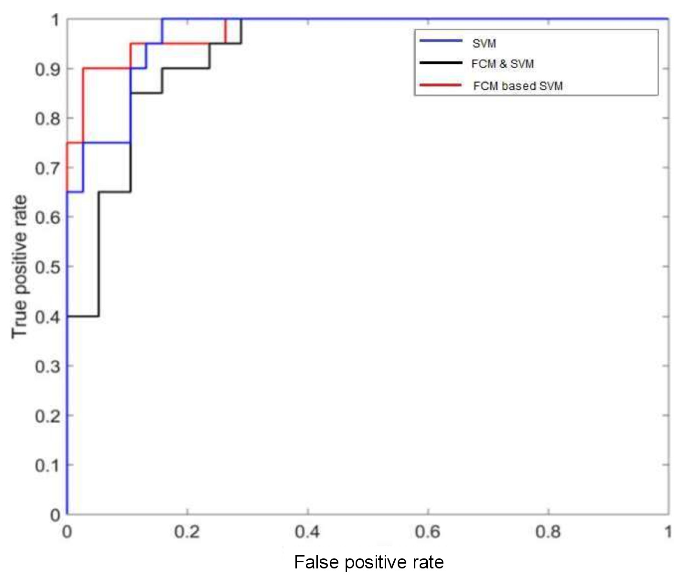
For evaluating the performance of mammographic tumor classification, receiver operating characteristics (ROC) curves and accuracy are measured by the proposed schemes. The ROC curve indicates the main contrast capacity of various methods. Apart from this, accuracy can also be measured for necessary significant evaluation. Accuracy is uttermost important because it provides precise rate of classification of two different levels (i.e., benign and malignant). It should be as high as possible for a classification model.
In Figure 4, the performance of different classifiers with the MIAS datasets is depicted with ROC plots using ‘ROCR’ package in R-software. The AUC can measure the performance of classification which is between 0 and 1. It summarizes the entire location of the ROC curve rather than depending on a specific operating point [31,32]. For FCM-based SVM method, the AUC is which indicates that it provides the best performance among all (from Figure 4). The accuracy of this method is . The reduction of error rate is compared with each of the proposed models. The performance of the model by ROC curve is also measured using estimation of the Area Under Curve (AUC) value.
AUC (based on ROC) and accuracy seems not the same concept. Accuracy is based on one specific cutpoint, while ROC tries to cover all the cutpoint and plots the sensitivity and specificity. Whenever we compare the overall accuracy, we are comparing the accuracy based on some cutpoint. The overall accuracy varies from different cutpoint. The area under the curve (AUC) is equal to the probability that a classifier will rank a randomly chosen positive instance higher than a randomly chosen negative example. It measures the classifiers skill in ranking a set of patterns according to the degree to which they belong to the positive class, but without actually assigning patterns to classes. The accuracy also depends on the ability of the classifier to rank patterns, but also on its ability to select a threshold in the ranking used to assign patterns to the positive class if above the threshold and to the negative class if below. Thus the classifier with the higher AUC is likely to also have a higher accuracy as the ranking of patterns which is beneficial to both AUC and accuracy. However, if one classifier ranks patterns well, but selects the threshold badly, it can have a high AUC but a poor accuracy. The high value of AUC indicates how strongly any predictor is capable for classification between two different classes of the response variable. Features with higher AUC are selected and overall performance of these features have been estimated by constructing a model using RF. It is observed that FCM based on SVM classification can maximize both AUC and accuracy.
The changing structure of cells can be recognized by analyzing the images obtained from mammogram method. Such images are very complex in nature and need fruitful information to analyse the malignancy properly. FCM method is used mainly for segmentation image to enhance the tumor’s shape. Although the SVM classification for breast cancer detection has achieved with high accuracy, but with FCM-based SVM method the accuracy rate is increased which provides that the rate of proposed method (FCM-based SVM) is higher than all previous methods. The success rate of SVM is but with the FCM-based SVM method, the success rates are increased to , shown in Table 5. After comparison of all underlying methods (described in Section 7 and Section 8), FCM-based SVM gives better accuracy than others proposed methods.
9. Concluding Remarks
Breast cancer (BC) is a very serious disease among women worldwide as it is accountable for increasing death rates among women. For improving the current era with BC is a vital concern and it can be achieved by fruitful diagnosis, proper investigation, appropriate patient, and with proper clinical management. To identify BC in the early stages, a regular basic check-up ca save many lives of human beings. The status of this cancer is changing with time since the distribution, appearance, and structural geometry of the cells change on a particular time basis due to the chemical changes which are always going on inside the cells. Due to the non trivial nature of the images the physician sometimes making a decision, might counter others. However, computer-aided-diagnosis methods can be enlightened a significant amount of information from the obtained images and also provide a proper decision based on the achieved information (viz., identification of cancer) using classifications of the images. Here, five various approaches including LDA were compared based on their performance in classifying the characters and classes of image data-set of breast cancer cells. First we demonstrated that classification accuracy can be increased in terms of both rate of misclassification and log-loss using SVM method which performs very well and slightly out performed NNET. Both (i.e., SVM and NNET) performed much better than RF, NPMR, and LDA.
The contribution of these methods is of utmost importance and using such advanced techniques with proposed modifications are used for image classification purpose, especially for image of breast cancer classification and also for segmentation. Overall SVM performs better than other underlying models, so additional extension has been taken into account in this current work with classifier ensembles. Then the further utilizations of FCM and SVM combination method and FCM based on the SVM method make a delightful scenario for the image classification. The comparison results among them provide higher accuracy, such enhancement confirms the effectiveness of the proposed approach for malignant tumor with the goal of increasing the accuracy.
Author Contributions
Conceptualization, S.G., G.S. and M.D.l.S.; Methodology, S.G., G.S. and M.D.l.S.; Investigation, S.G., G.S. and M.D.l.S.; Formal analysis, S.G., G.S. and M.D.l.S.; Writing—original draft preparation, S.G., G.S. and M.D.l.S.; Writing—review and editing, S.G., G.S. and M.D.l.S. All authors have read and agreed to the published version of the manuscript.
Funding
This research was funded by the Spanish Government for its support through grant RTI2018-094336-B-100 (MCIU/AEI/FEDER, UE) and to the Basque Government for its support through grant IT1207-19.
Institutional Review Board Statement
Not applicable.
Informed Consent Statement
Not applicable.
Data Availability Statement
The data used to support the findings of this study are included in the references within the article.
Acknowledgments
The authors are grateful to the anonymous referees and Editors for their careful reading, valuable comments and helpful suggestions, which have helped them to improve the presentation of this work significantly. The third author (Manuel De la Sen) is grateful to the Spanish Government for its support through grant RTI2018-094336-B-100 (MCIU/AEI/FEDER, UE) and to the Basque Government for its support through grant IT1207-19.
Conflicts of Interest
The authors declare that they have no conflict of interest regarding this work.
References
- Facts and Figures. 2017–2018. Available online: https://www.cancer.org/research/cancer-facts-statistics8 (accessed on 5 March 2018).
- Bezdek, J.C. Pattern Recognition with Fuzzy Objective Function Algorithms; Springer Science and Business Media: Berlin, Germany, 2013. [Google Scholar]
- Ghosh, S.; Samanta, G.P. Statistical modelling for cancer mortality. In Letters in Biomathemtics; Taylor and Francies: Abingdon, UK, 2019; Volume 6. [Google Scholar] [CrossRef] [Green Version]
- Howlader, N.; Noone, A.M.; Krapcho, M. SEER Cancer Statistics Review, 1975–2014; National Cancer Institute: Bethesda, MD, USA, 2017. [Google Scholar]
- Cancer—WHO Fact Sheets. 2017. Available online: http://www.who.int/mediacentre/factsheets/fs297/en/ (accessed on 14 October 2017).
- Sickles, E.A. Breast masses: Mammographic evaluation. Radiology 1989, 173, 297–330. [Google Scholar] [CrossRef] [PubMed]
- Mohanty, F.; Rup, S.; Dash, B.; Majhi, B.; Swamy, M. Mammogram classification using contourlet features with forest optimization-based feature selection approach. Multimed. Tools Appl. 2018, 78, 12805–12834. [Google Scholar] [CrossRef]
- Cawley, G.C.; Talbot, N.L. On over-fitting in model selection and subsequent selection bias in performance evaluation. J. Mach. Learn. Res. 2010, 11, 2079–2107. [Google Scholar]
- Gorgel, P.; Sertbas, A.; Uçan, O.N. Computer-aided classification of breast masses in mammogram images based on spherical wavelet transform and support vector machines. Expert Syst. 2015, 32, 155–164. [Google Scholar] [CrossRef]
- MIAS Database. 2012. Available online: http://peipa.essex.ac.uk/info/mias.html (accessed on 11 December 2012).
- Feig, S.A.; Yaffe, M.J. Digital mammography, computer-aided diagnosis, and telemammography. Radiol. Clin. N. Am. 1995, 33, 1205–1230. [Google Scholar] [PubMed]
- James, A.P.; Sugathan, S. Parallel Realization of Cognitive Cells on Film Mammography. In Proceedings of the 12th IEEE International Conference on Trust, Security and Privacy in Computing and Communications, Melbourne, Australia, 16–18 July 2013. [Google Scholar]
- Chuang, K.S.; Tzeng, H.L.; Chen, S.; Wu, J.; Chen, T.J. Fuzzy c-means clustering with spatial information for image segmentation computerized medical imaging and graphics. Comput. Med. Imaging Graph. 2006, 30, 9–15. [Google Scholar] [CrossRef] [PubMed] [Green Version]
- Keller, B.; Nathan, D.; Wang, Y.; Zheng, Y.; Gee, J.; Conant, E.; Kontos, D. Adaptive multi-cluster fuzzy c means segmentation of breast parenchymal tissue in digital mammography. In International Conference on Medical Image Computing and Computer-Assisted Intervention; Springer: Toronto, ON, Canada, 2011; pp. 562–569. [Google Scholar]
- Johnson, R.A.; Wichern, D. Applied Multivariate Statistical Analysis, 6th ed.; Prentice Hall: Englewood Cliffs, NJ, USA, 2002. [Google Scholar]
- Fisher, R.A. The use of multiple measurements in taxonomic problems. Ann. Eugen. 1936, 7, 179–188. [Google Scholar] [CrossRef]
- Hastie, T.; Tibshirani, R.; Friedman, J. The Elements of Statistical Learning: Data Mining, Inference and Prediction, 1st ed.; Springer: New York, NY, USA, 2001. [Google Scholar]
- Breiman, L. Random forests. Mach. Learn. 2001, 45, 5–32. [Google Scholar] [CrossRef] [Green Version]
- Everson, T.M.; Lyons, G.; Zhang, H.; Soto-Ramirez, N.; Lockett, G.A.; Patil, V.K.; Merid, S.K.; Soderhall, C.; Melen, E.; Holloway, J.W.; et al. DNA methylation loci associated with atopy and high serum IgE: A genome-wide application of recursive Random Forest feature selection. Genome Med. 2015, 7, 89. [Google Scholar] [CrossRef] [PubMed] [Green Version]
- Efron, B. Bootstrap methods: Another look at the jackknife. Ann. Stat. 1979, 7, 1–26. [Google Scholar] [CrossRef]
- Boser, B.E.; Guyon, I.M.; Vapnik, V.N. A training algorithm for optimal margin classifiers. In Proceedings of the 5th Annual ACM Workshop on Computational Learning Theory, Pittsburgh, PA, USA, 27–29 July 1992; ACM Press: New York, NY, USA, 1992; pp. 144–152. [Google Scholar]
- Chang, C.; Lin, C. LIBSVM: A library for support vector machine. ACM Trans. Intell. Syst. Technol. 2011, 2. [Google Scholar] [CrossRef]
- Venables, W.N.; Ripley, B.D. Modern Applied Statistics with S, 4th ed.; Springer: New York, NY, USA, 2002. [Google Scholar]
- Powers, S.; Hastie, T.; Tibshirani, R. Nuclear penalized multinomial regression with an application to predicting at bat outcomes in baseball. Stat. Model. 2016, 18, 388–410. [Google Scholar] [CrossRef] [PubMed]
- Stoica, P.; Selen, Y.; Li, J. Multi-model approach to model selection. Digit. Signal Process. 2004, 14, 399–412. [Google Scholar] [CrossRef]
- Lin, G.; Chawla, M.K.; Olson, K.; Barnes, C.A.; Guzowski, J.F.; Bjornsson, C.; Shain, W.; Roysam, B. A Multi-Model Approach to Simultaneous Segmentation and Classification of Heterogeneous Populations of Cell Nuclei in 3D Confocal Microscope Images. Cytom. Part A 2007, 71, 724–736. [Google Scholar] [CrossRef] [PubMed]
- Breiman, L. Bagging predictors. Mach. Learn. 1996, 24, 123–140. [Google Scholar] [CrossRef] [Green Version]
- Kim, H.C.; Pang, S.; Je, H.M.; Kim, D.; Bang, S.Y. Constructing support vector machine ensemble. Pattern Recognit. 2003, 36, 2757–2767. [Google Scholar] [CrossRef]
- Schapire, R.E. The strength of weak learnabilty. Mach. Learn. 1990, 5, 197–227. [Google Scholar] [CrossRef] [Green Version]
- Hoppner, F.; Klawonn, F.; Kruse, R.; Runkler, T. Fuzzy Cluster Analysis: Methods for Classification, Data Analysis and Image Recognition; Wiley: New York, NY, USA, 1999. [Google Scholar]
- Hanley, J.A.; McNeil, B.J. The meaning and use of the area under a receiver operating characteristic (ROC) curve. Radiology 1982, 143, 29–36. [Google Scholar] [CrossRef] [PubMed] [Green Version]
- Swets, J.A. ROC analysis applied to the evaluation of medical imaging techniques. Investig. Radiol. 1979, 14, 109–121. [Google Scholar] [CrossRef]
Figure 1.
Structure of support vector machine.
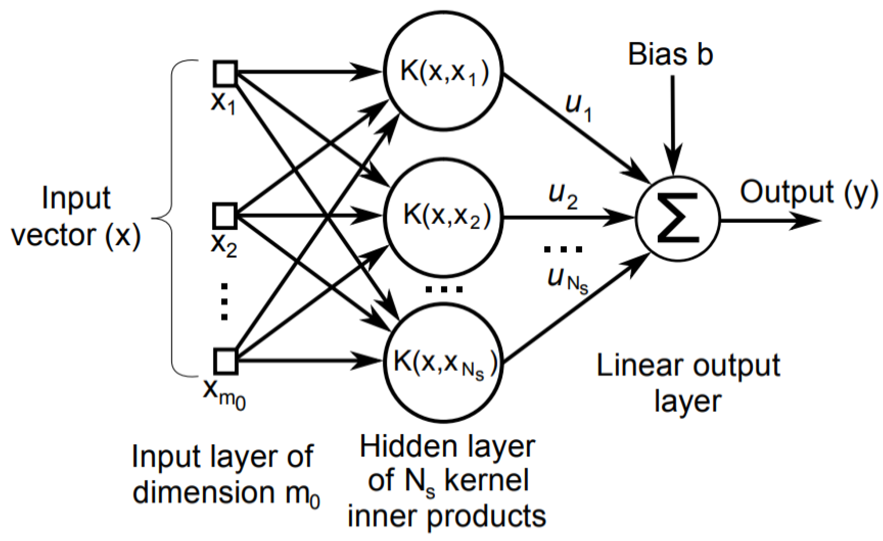
Figure 2.
Block scheme for FCM and SVM combinatione.
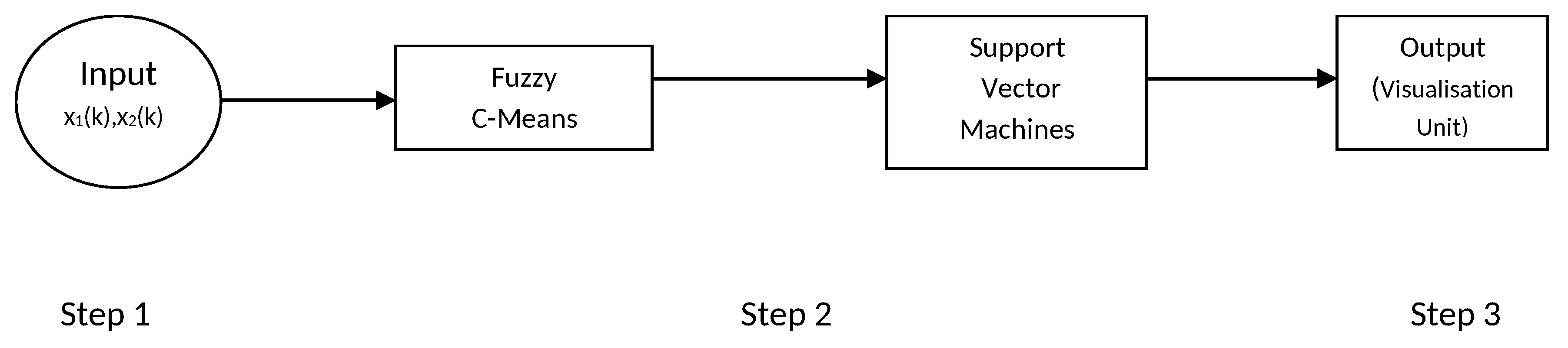
Figure 3.
Block scheme for FCM-based SVM.

Figure 4.
ROC curve.

Table 1.
Logloss comparison.
| Character | Class | ||||||||||
|---|---|---|---|---|---|---|---|---|---|---|---|
| LDA | RF | SVM | NPMR | NNET | LDA | RF | SVM | NPMR | NNET | ||
| Centre | 1.341 | 0.331 | 0.329 | 0.357 | 0.343 | 3.450 | 0.845 | 0.796 | 0.802 | 0.811 | |
| Centre | 1.653 | 0.325 | 0.321 | 0.328 | 0.321 | 3.454 | 0.787 | 0.728 | 0.884 | 0.741 | |
| 1.047 | 0.335 | 0.271 | 0.335 | 0.326 | 3.353 | 0.829 | 0.829 | 0.81 | 0.829 | ||
| Centre | 1.012 | 0.332 | 0.338 | 0.355 | 0.330 | 3.279 | 0.997 | 0.988 | 0.992 | 1.002 | |
| Centre | 1.271 | 0.323 | 0.318 | 0.373 | 0.363 | 2.822 | 0.977 | 0.982 | 0.985 | 1.002 | |
| 1.093 | 0.327 | 0.298 | 0.348 | 0.320 | 3.103 | 0.976 | 0.957 | 0.959 | 1.003 | ||
Table 2.
Accuracy comparison.
| Character | Class | ||||||||||
|---|---|---|---|---|---|---|---|---|---|---|---|
| LDA | RF | SVM | NPMR | NNET | LDA | RF | SVM | NPMR | NNET | ||
| Centre | 0.812 | 0.833 | 0.898 | 0.857 | 0.877 | 0.745 | 0.789 | 0.896 | 0.889 | 0.895 | |
| Centre | 0.778 | 0.899 | 0.936 | 0.908 | 0.901 | 0.654 | 0.799 | 0.829 | 0.818 | 0.829 | |
| 0.747 | 0.845 | 0.885 | 0.835 | 0.826 | 0.618 | 0.780 | 0.785 | 0.781 | 0.784 | ||
| Centre | 0.882 | 0.889 | 0.921 | 0.891 | 0.885 | 0.779 | 0.835 | 0.851 | 0.833 | 0.849 | |
| Centre | 0.828 | 0.843 | 0.895 | 0.879 | 0.863 | 0.582 | 0.866 | 0.882 | 0.850 | 0.882 | |
| 0.821 | 0.839 | 0.841 | 0.843 | 0.820 | 0.701 | 0.853 | 0.857 | 0.849 | 0.857 | ||
Table 3.
Classification accuracies of single SVM and SVM ensembles.
| Classification | Methods | Accuracy in Percentage |
|---|---|---|
| SVM | Single | 87.258 |
| Bagging | 89.323 | |
| Boosting | 88.575 |
Table 4.
Confusion matrix for two classes classification.
| Predicted Positive | Predicted Negative | |
|---|---|---|
| Actual positive | TP | FN |
| Actual negative | FP | TN |
Table 5.
Performance evaluation and comparisonn.
| Methods | Accuracy in Percentage | Error Rate |
|---|---|---|
| SVM | 87.258 | 0.127 |
| FCM & SVM | 82.33 | 0.177 |
| FCM based SVM | 91.39 | 0.086 |
Publisher’s Note: MDPI stays neutral with regard to jurisdictional claims in published maps and institutional affiliations. |
© 2021 by the authors. Licensee MDPI, Basel, Switzerland. This article is an open access article distributed under the terms and conditions of the Creative Commons Attribution (CC BY) license (https://creativecommons.org/licenses/by/4.0/).
Share and Cite
MDPI and ACS Style
Ghosh, S.; Samanta, G.; De la Sen, M. Multi-Model Approach and Fuzzy Clustering for Mammogram Tumor to Improve Accuracy. Computation 2021, 9, 59. https://0-doi-org.brum.beds.ac.uk/10.3390/computation9050059
AMA Style
Ghosh S, Samanta G, De la Sen M. Multi-Model Approach and Fuzzy Clustering for Mammogram Tumor to Improve Accuracy. Computation. 2021; 9(5):59. https://0-doi-org.brum.beds.ac.uk/10.3390/computation9050059
Chicago/Turabian StyleGhosh, Sarada, Guruprasad Samanta, and Manuel De la Sen. 2021. "Multi-Model Approach and Fuzzy Clustering for Mammogram Tumor to Improve Accuracy" Computation 9, no. 5: 59. https://0-doi-org.brum.beds.ac.uk/10.3390/computation9050059
Note that from the first issue of 2016, this journal uses article numbers instead of page numbers. See further details here.