
Framework for Predicting Failure in Polymeric Unidirectional Composites through Combined Experimental and Computational Mesoscale Modeling Techniques

Abstract
:1. Introduction
2. Composite Constituent Properties
2.1. Carbon Fiber Properties
2.2. Epoxy Matrix Properties
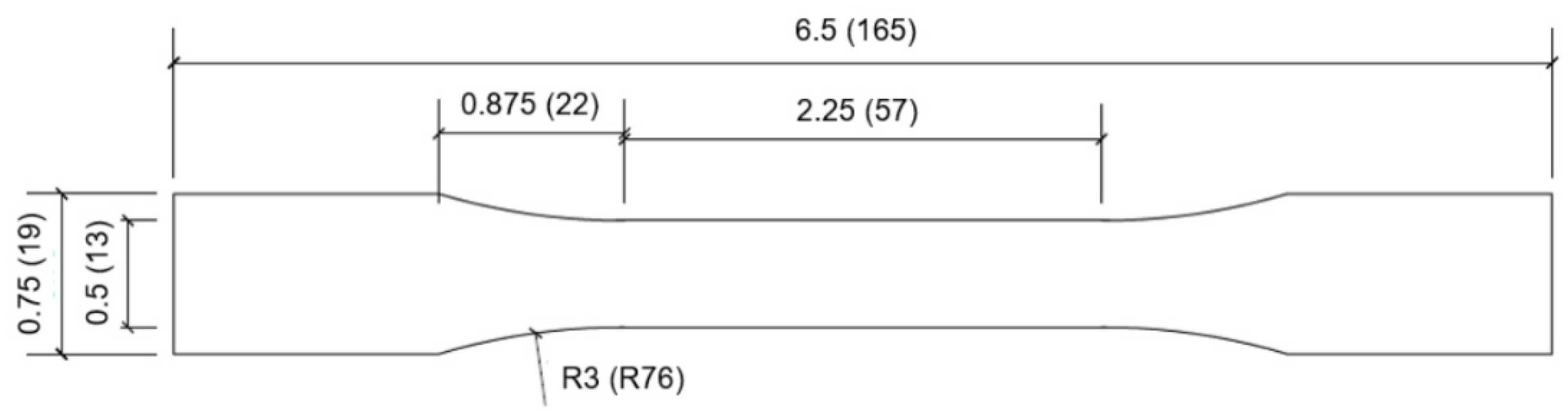
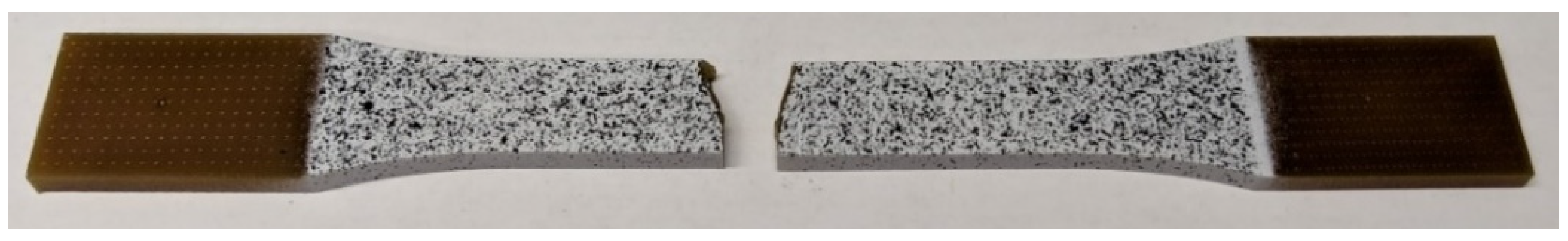
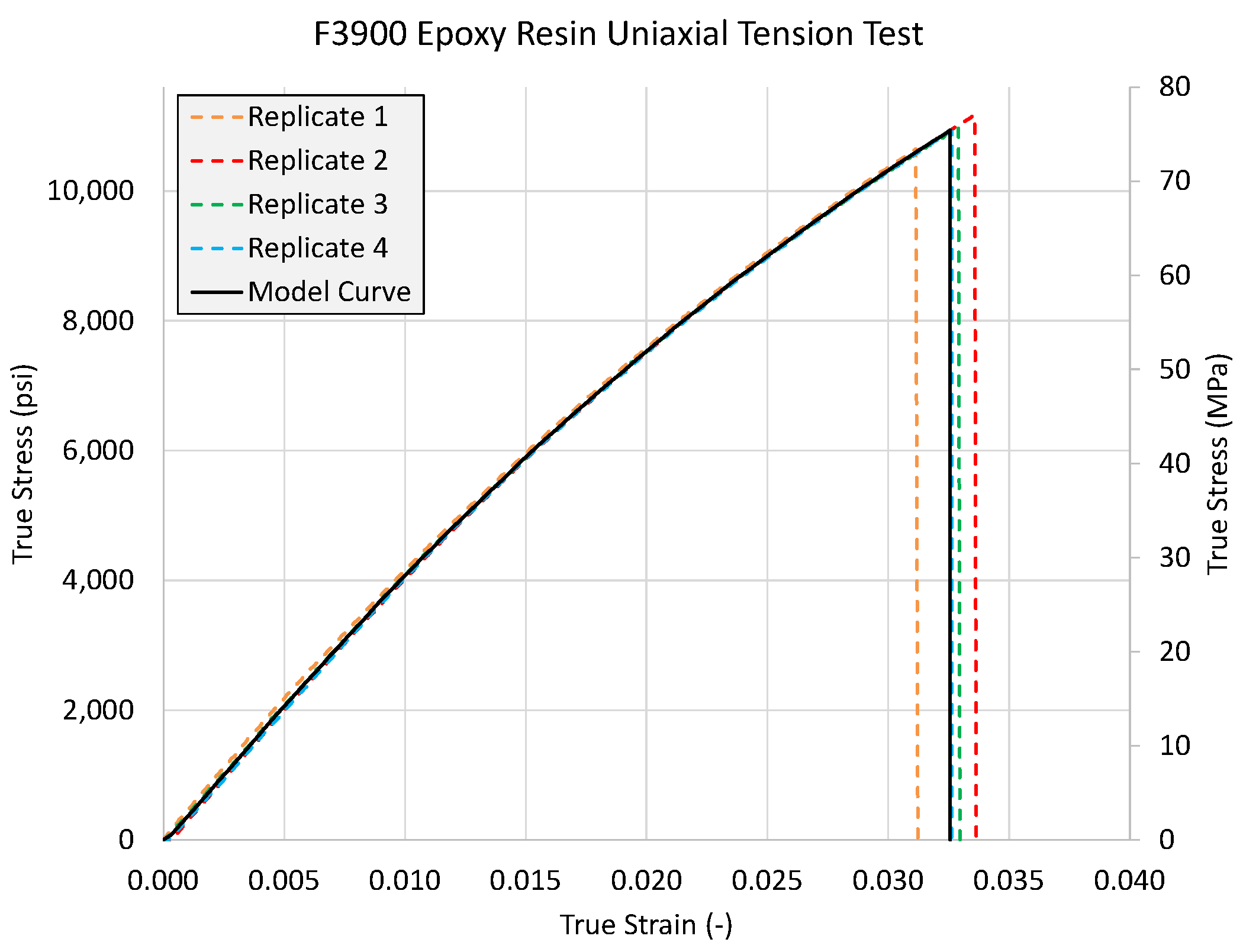
2.2.1. Tension Tests
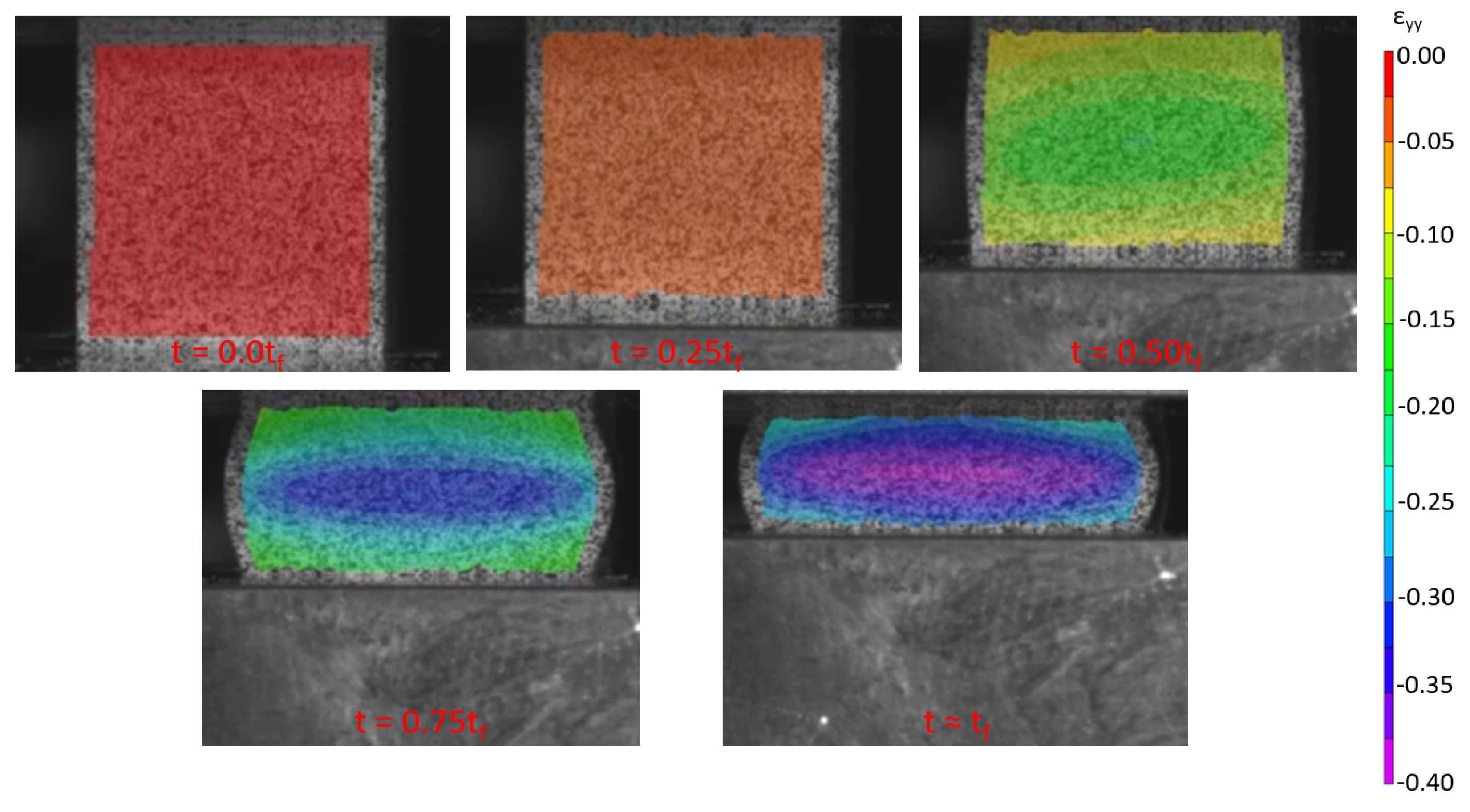
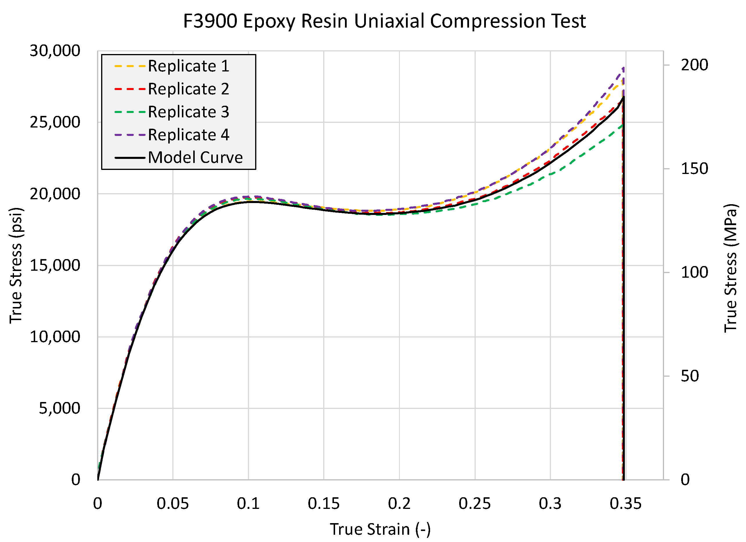
2.2.2. Compression Tests
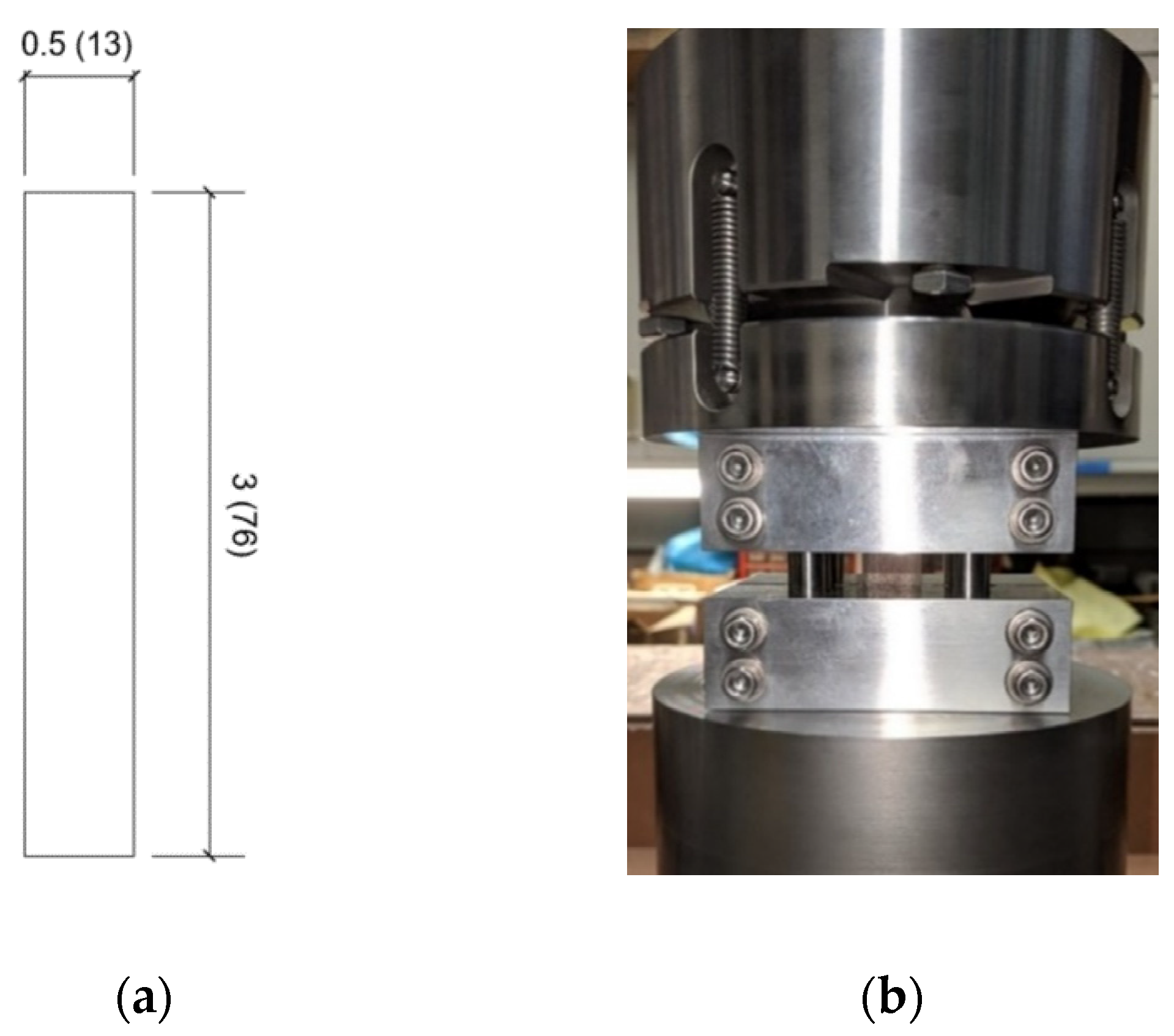
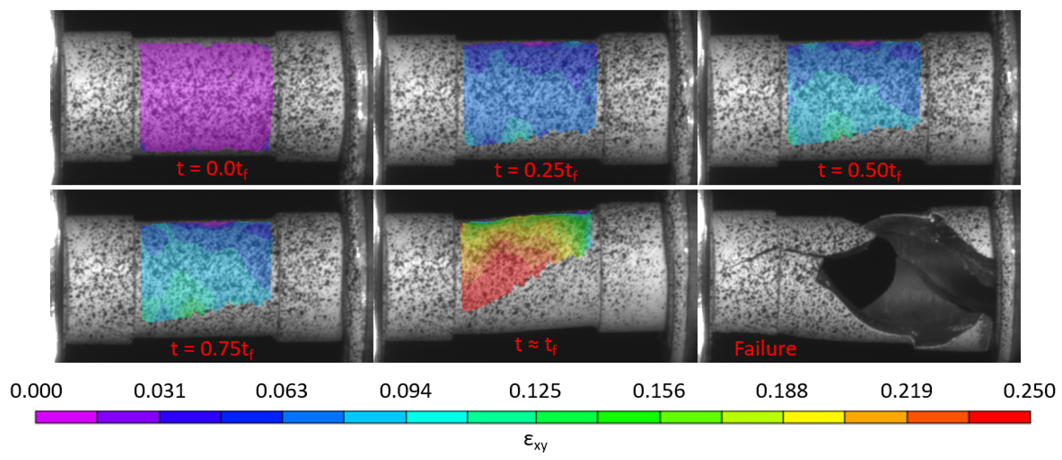
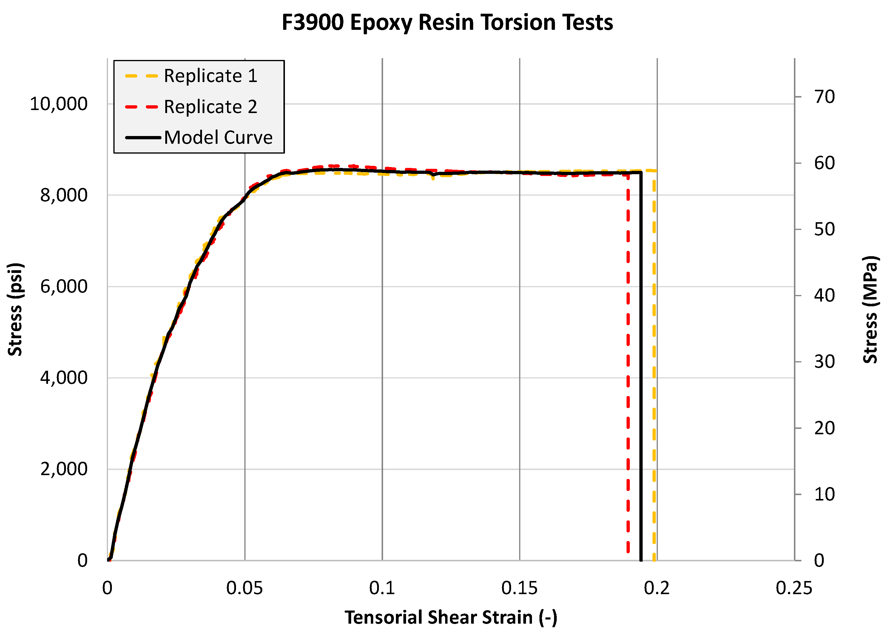
2.2.3. Shear Tests
2.2.4. Remaining Input Data
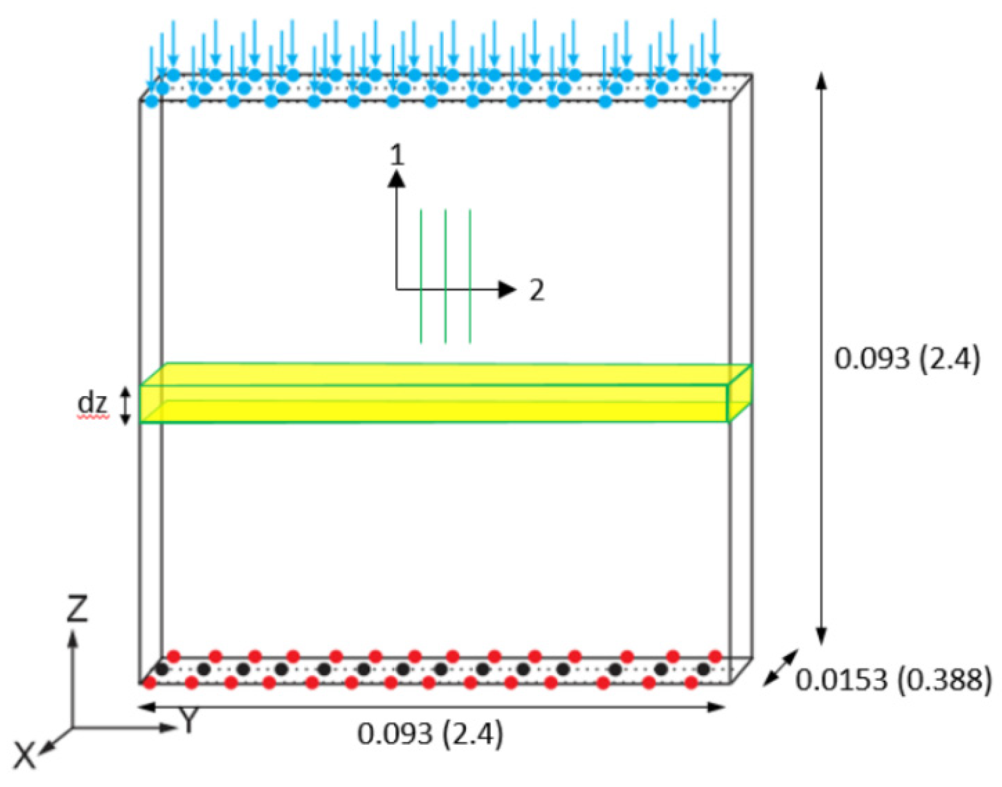
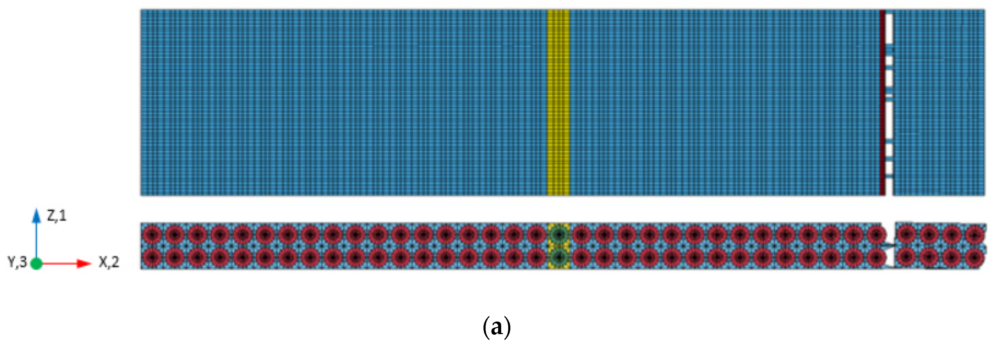
3. Finite Element Modeling of the Unidirectional Composite
Virtual Test Models
4. Virtual Test Results
4.1. Calibration and Verification of Matrix Data Using T800-F3900 Composite Data
4.2. Calibration and Verification of Fiber Data
4.3. Validation of the Material Models
4.3.1. 1-Direction Tension Test
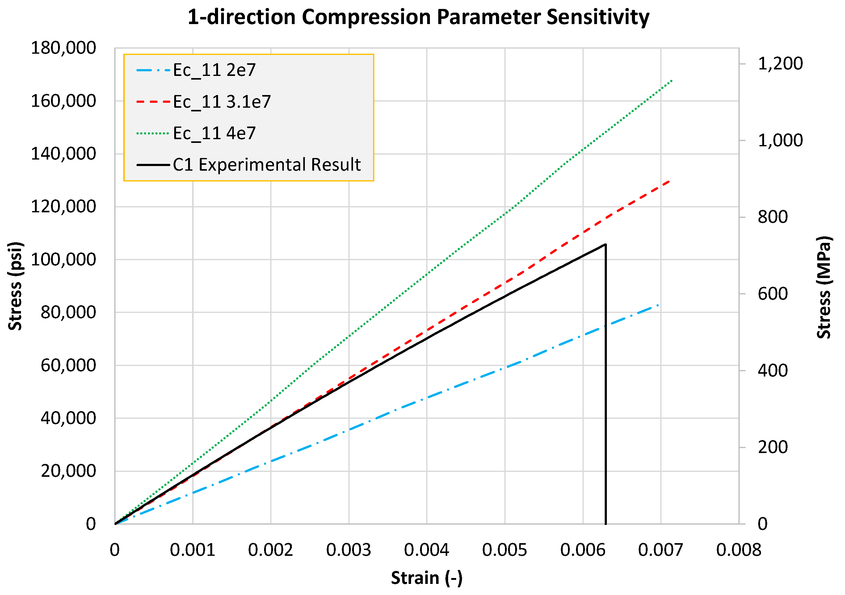
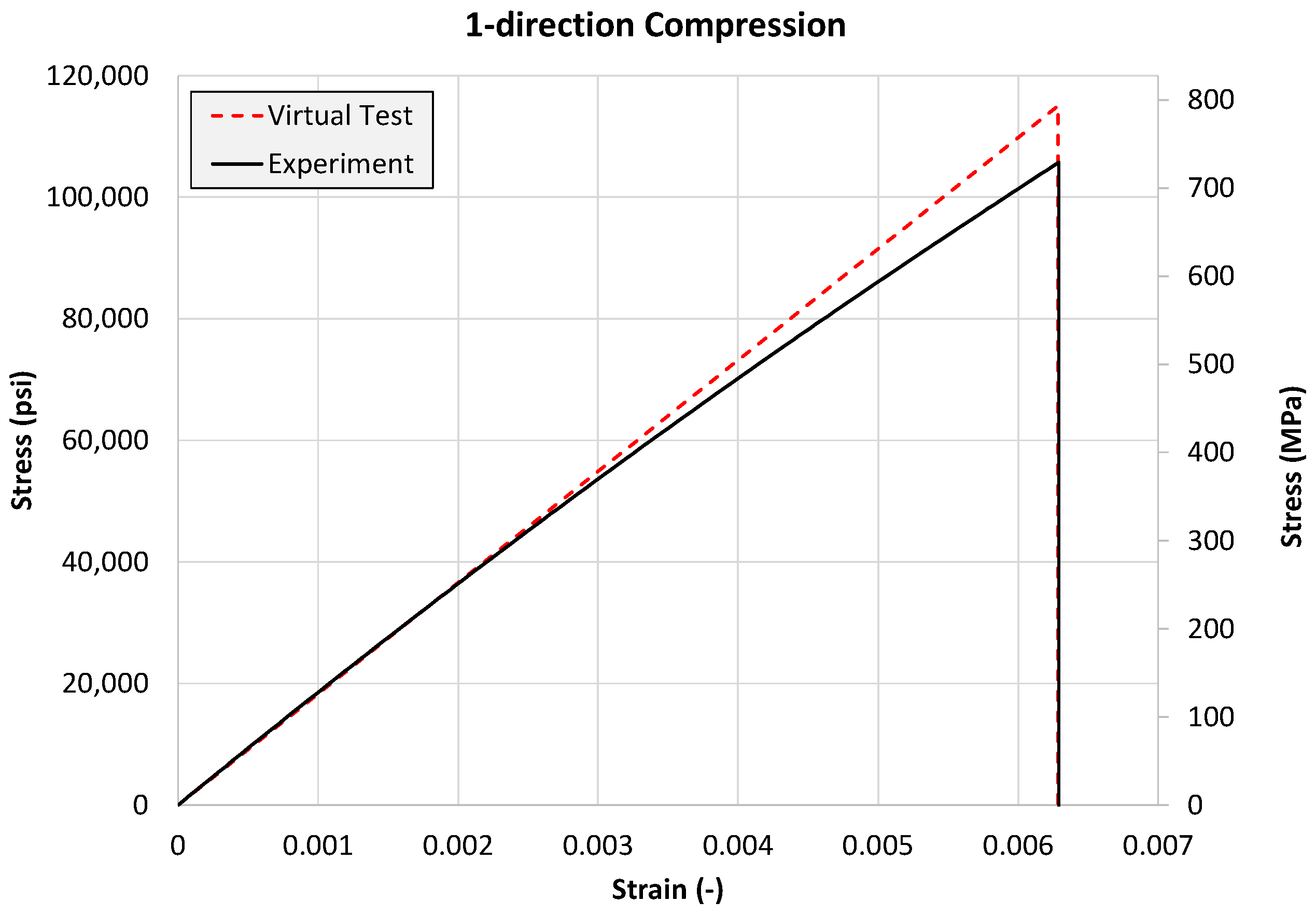
4.3.2. 1-Direction Compression Test
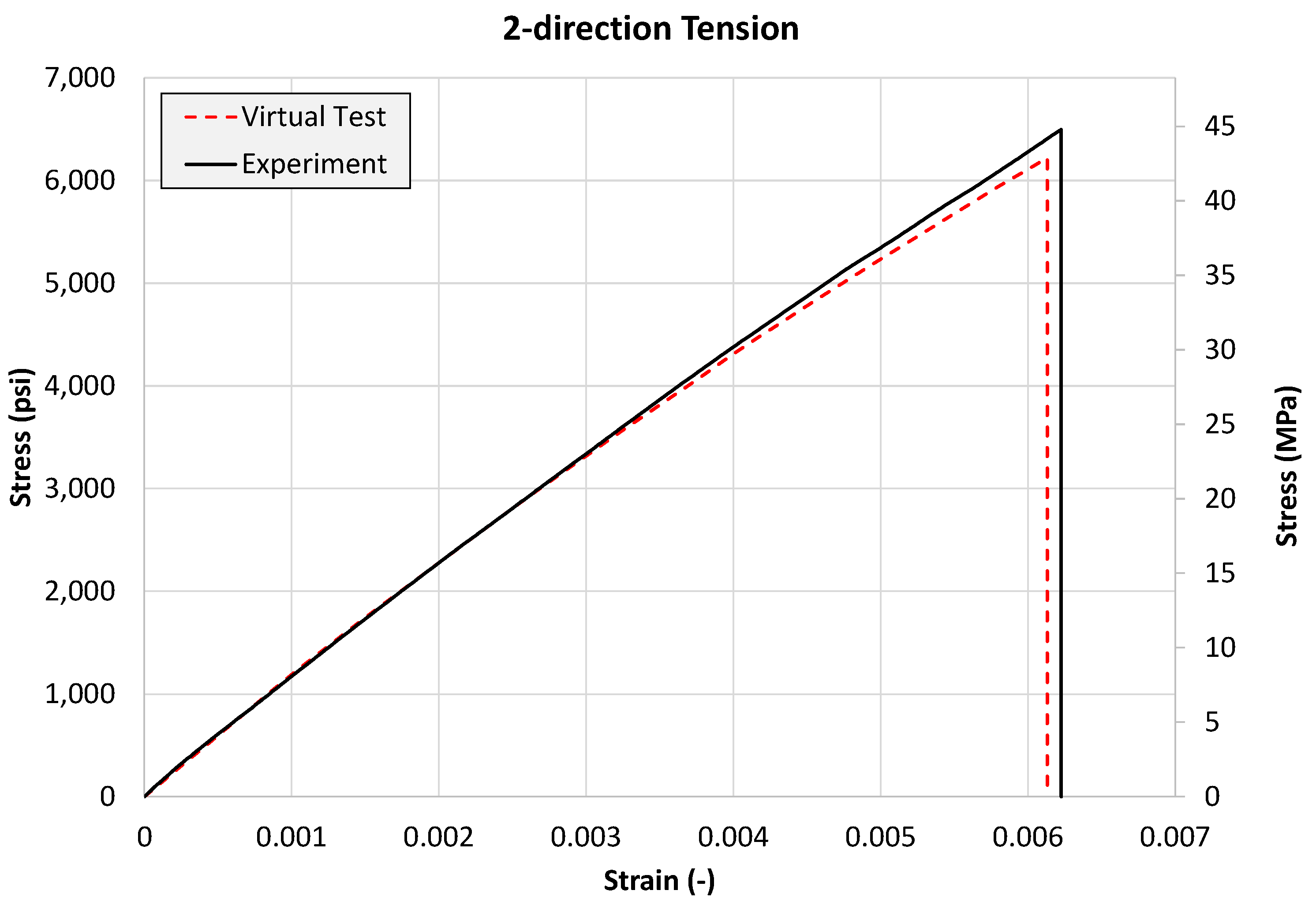
4.3.3. 2-Direction Tension Test
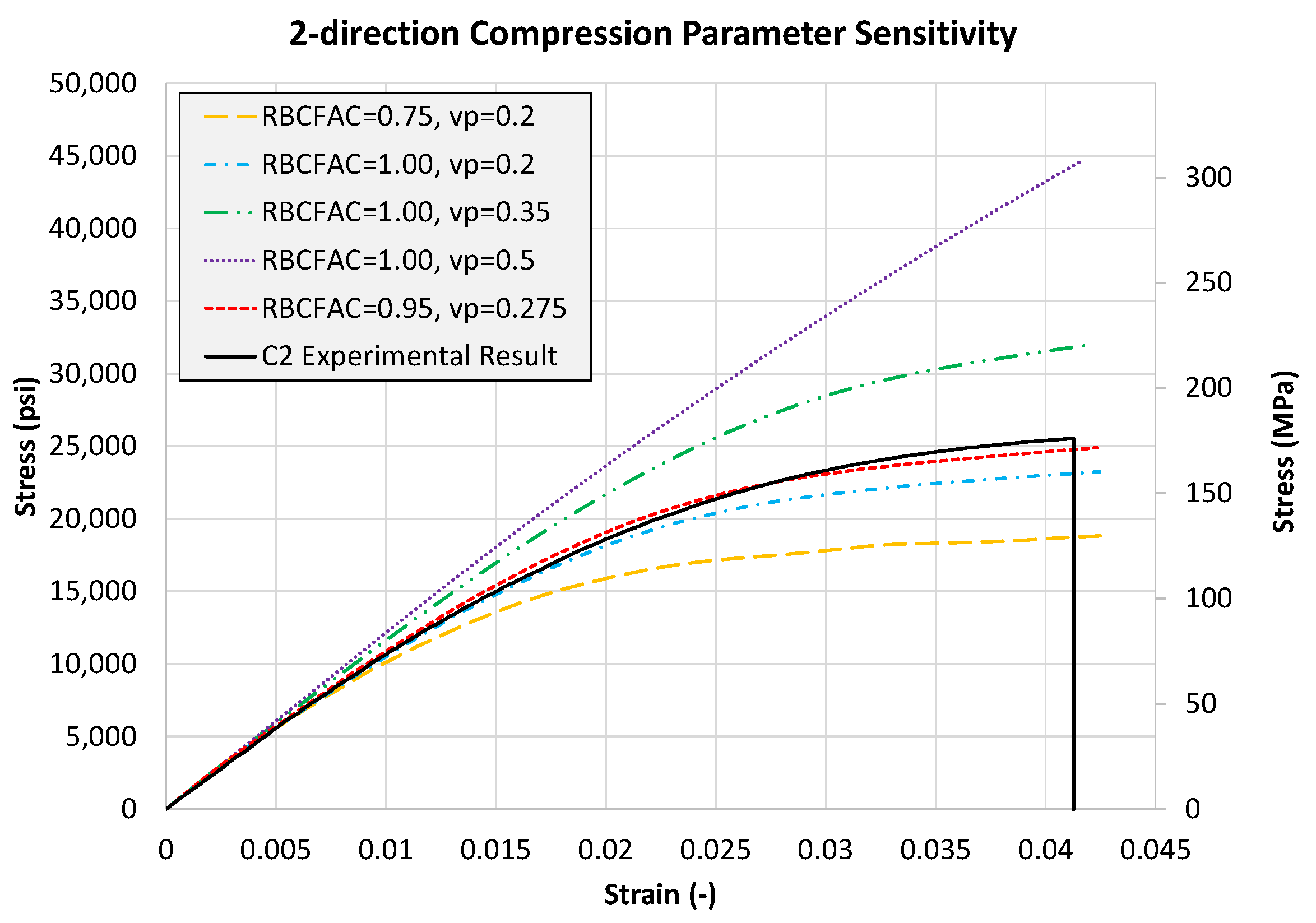
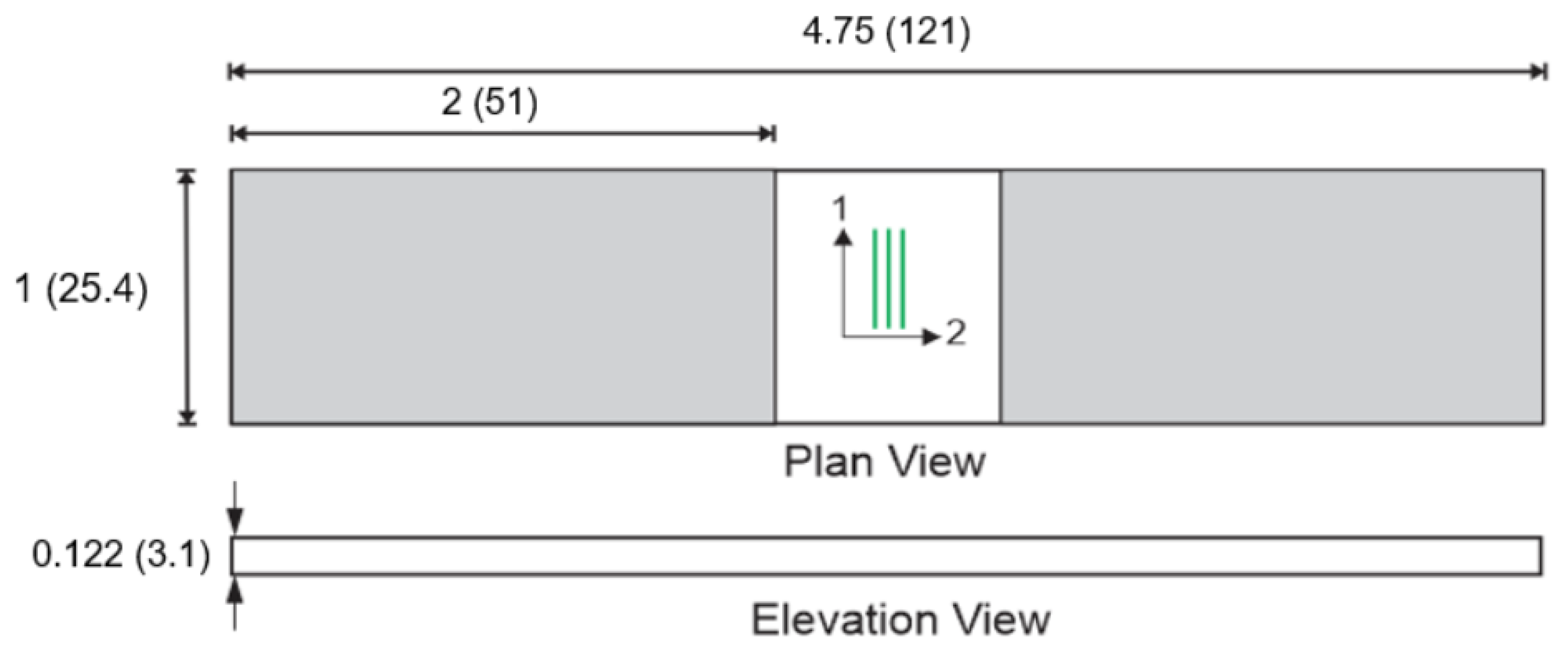
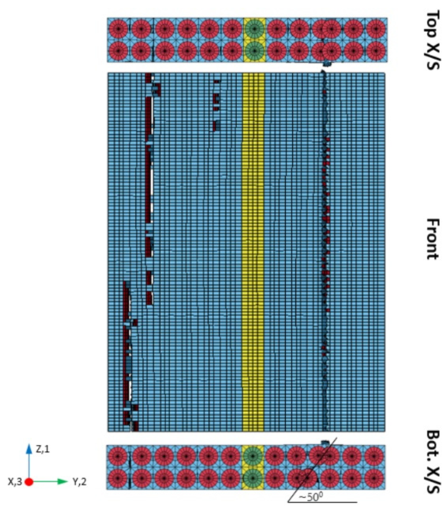
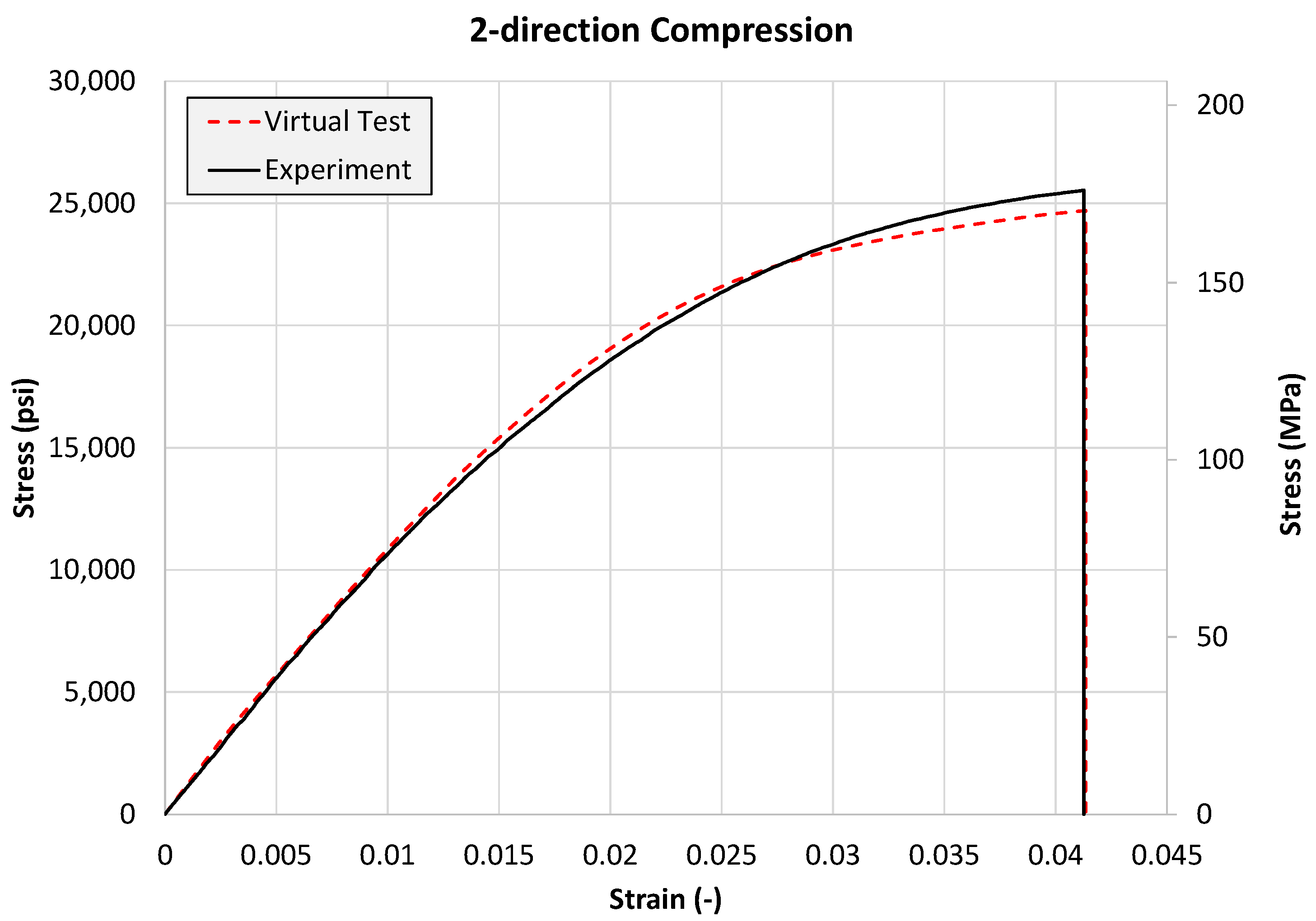
4.3.4. 2-Direction Compression Test
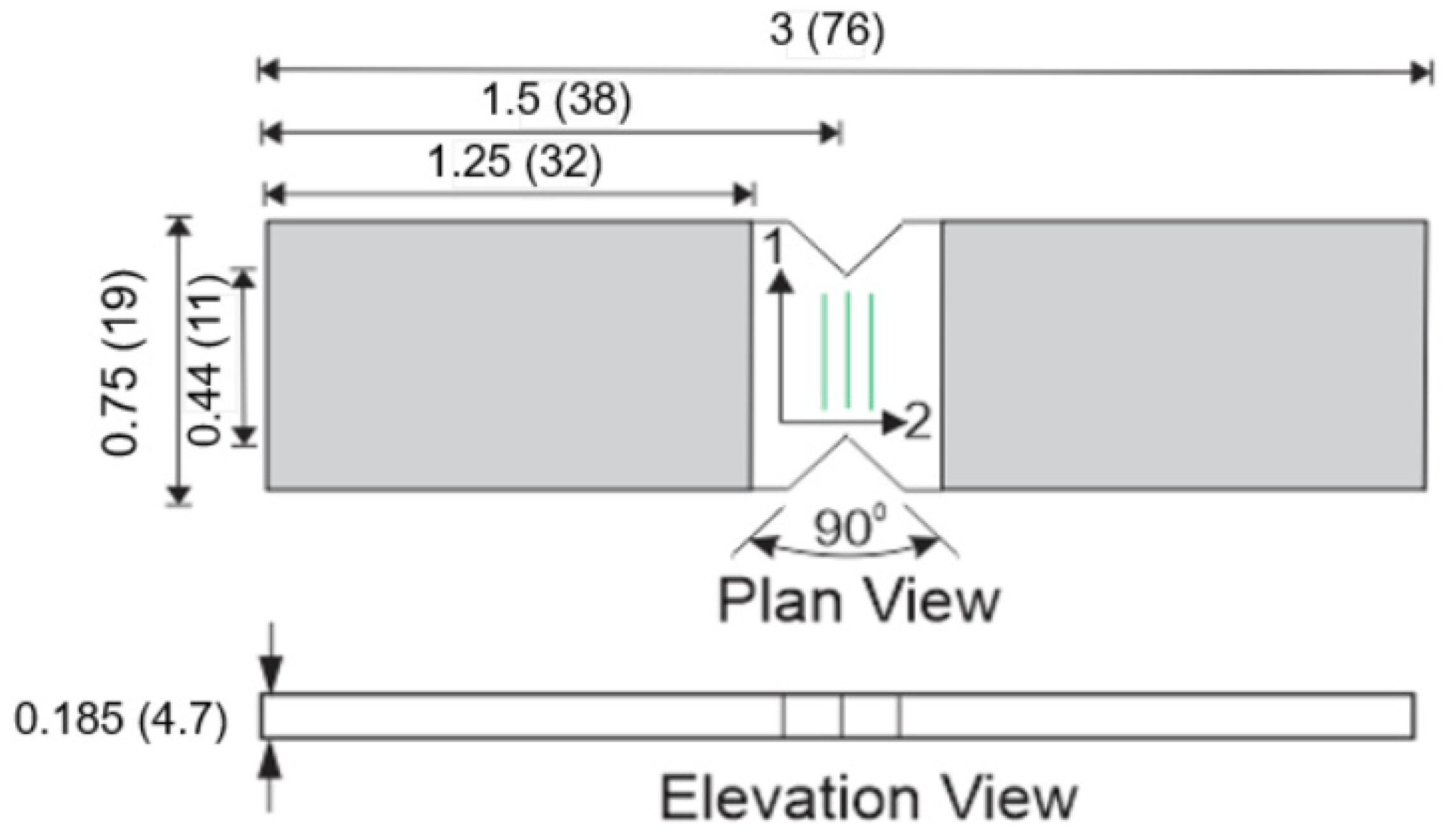
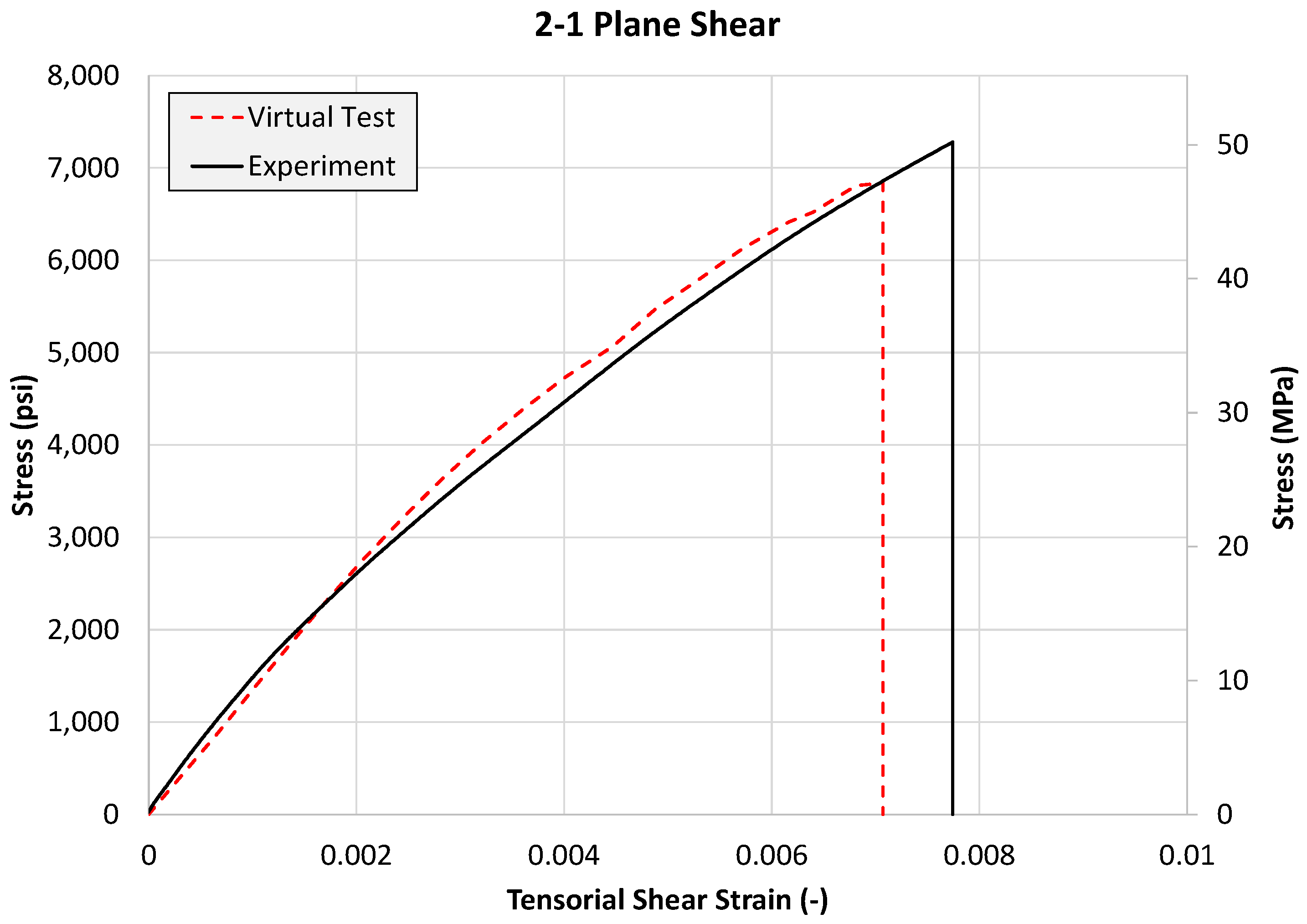
4.3.5. 2-1 Plane Shear Test
5. Concluding Remarks
Author Contributions
Funding
Informed Consent Statement
Data Availability Statement
Acknowledgments
Conflicts of Interest
Appendix A

References
- Hinton, M.; Kaddour, A. The background to the Second World-Wide Failure Exercise. J. Compos. Mater. 2012, 46, 2283–2294. [Google Scholar] [CrossRef]
- Kaddour, A.S.; Hinton, M. Failure Criteria for Composites. In Reference Module in Materials Science and Materials Engineering; Elsevier: Amsterdam, The Netherlands, 2017. [Google Scholar] [CrossRef]
- Midani, M.; Seyam, A.; Pankow, M. A Generalized Analytical Model for Predicting the Tensile Behavior of 3D Orthogonal Woven Composites Using Finite Deformation Approach. J. Text. Inst. 2018, 109, 1465–1476. [Google Scholar] [CrossRef]
- Harrington, J.; Hoffarth, C.; Rajan, S.D.; Goldberg, R.K.; Carney, K.S.; Dubois, P.; Blankenhorn, G. Using Virtual Tests to Complete the Description of a Three-Dimensional Orthotropic Material. J. Aerosp. Eng. 2017, 30, 04017025. [Google Scholar] [CrossRef]
- Vogler, T.; Kyriakides, S. Inelastic behavior of an AS4/PEEK composite under combined transverse compression and shear. Part I: Experiments. Int. J. Plast. 1999, 15, 783–806. [Google Scholar] [CrossRef]
- Zinoviev, P.A.; Tsvetkov, S.V.; Kulish, G.G.; van den Berg, R.W.; Van Schepdael, L.J.M.M. The behavior of high-strength unidirectional composites under tension with superposed hydrostatic pressure. Compos. Sci. Technol. 2001, 61, 1151–1161. [Google Scholar] [CrossRef]
- Hine, P.; Duckett, R.; Kaddour, A.; Hinton, M.; Wells, G. The effect of hydrostatic pressure on the mechanical properties of glass fibre/epoxy unidirectional composites. Compos. Part A Appl. Sci. Manuf. 2005, 36, 279–289. [Google Scholar] [CrossRef]
- Cai, D.; Zhou, G.; Silberschmidt, V.V. Effect of through-thickness compression on in-plane tensile strength of glass/epoxy composites: Experimental study. Polym. Test. 2016, 49, 1–7. [Google Scholar] [CrossRef] [Green Version]
- Daniel, I.M.; Luo, J.-J.; Schubel, P.M.; Werner, B.T. Interfiber/interlaminar failure of composites under multi-axial states of stress. Compos. Sci. Technol. 2009, 69, 764–771. [Google Scholar] [CrossRef]
- Canal, L.P.; Segurado, J.; LLorca, J. Failure surface of epoxy-modified fiber-reinforced composites under transverse tension and out-of-plane shear. Int. J. Solids Struct. 2009, 46, 2265–2274. [Google Scholar] [CrossRef] [Green Version]
- Melro, A.; Camanho, P.; Pires, F.; Pinho, S. Micromechanical analysis of polymer composites reinforced by unidirectional fibres: Part II—Micromechanical analyses. Int. J. Solids Struct. 2013, 50, 1906–1915. [Google Scholar] [CrossRef] [Green Version]
- Melro, A.R.; Camanho, P.P.; Andrade Pires, F.M.; Pinho, S.T. Micromechanical analysis of polymer composites reinforced by unidirectional fibres: Part I—Constitutive modelling. Int. J. Solids Struct. 2013, 50, 1897–1905. [Google Scholar] [CrossRef] [Green Version]
- Totry, E.; González, C.; LLorca, J. Prediction of the failure locus of C/PEEK composites under transverse compression and longitudinal shear through computational micromechanics. Compos. Sci. Technol. 2008, 68, 3128–3136. [Google Scholar] [CrossRef] [Green Version]
- Vaughan, T.J. Micromechanical Modelling of Damage and Failure in Fibre Reinforced Composites under Loading in the Transverse Plane. Ph.D. Dissertation, University of Limerick, Limerick, Ireland, 2011. [Google Scholar]
- Goldberg, R.K.; Carney, K.S.; DuBois, P.; Hoffarth, C.; Khaled, B.; Shyamsunder, L.; Rajan, S.D.; Blankenhorn, G. Implementation of a tabulated failure model into a generalized composite material model. J. Compos. Mater. 2018, 52, 3445–3460. [Google Scholar] [CrossRef]
- Shyamsunder, L.; Khaled, B.; Rajan, S.D.; Blankenhorn, G. Improving failure sub-models in an orthotropic plasticity-based material model. J. Compos. Mater. 2020. [Google Scholar] [CrossRef]
- Ansys-LST. Available online: http://lstc.com/ (accessed on 16 October 2020).
- Khaled, B.; Shyamsunder, L.; Hoffarth, C.; Rajan, S.D.; Goldberg, R.K.; Carney, K.S.; DuBois, P.; Blankenhorn, G. Experimental characterization of composites to support an orthotropic plasticity material model. J. Compos. Mater. 2018, 52, 1847–1872. [Google Scholar] [CrossRef]
- Achstetter, T. Development of A Composite Shell-Element Model for Impact Applications. Ph.D. Dissertation, George Mason University, Fairfax, VA, USA, 2019. [Google Scholar]
- Hoffarth, C. A Generalized Orthotropic Elasto-Plastic Material Model for Impact Analysis. Ph.D. Dissertation, Arizona State University, Tempe, AZ, USA, 2016. [Google Scholar]
- Hoffarth, C.; Rajan, S.D.; Goldberg, R.K.; Revilock, D.; Carney, K.S.; DuBois, P.; Blankenhorn, G. Implementation and validation of a three-dimensional plasticity-based deformation model for orthotropic composites. Compos. Part A Appl. Sci. Manuf. 2016, 91, 336–350. [Google Scholar] [CrossRef]
- Khaled, B. Experimental Characterization and Finite Element Modeling of Composites to Support a Generalized Orthotropic Elasto-Plastic Damage Material Model for Impact Analysis. Ph.D. Dissertation, Arizona State University, Tempe, AZ, USA, 2019. [Google Scholar]
- Shyamsunder, L.; Khaled, B.; Rajan, S.D.; Goldberg, R.K.; Carney, K.S.; DuBois, P.; Blankenhorn, G. Implementing deformation, damage, and failure in an orthotropic plastic material model. J. Compos. Mater. 2020, 54, 463–484. [Google Scholar] [CrossRef]
- Waterbury, M.C.; Drzal, L.T. On the Determination of Fiber Strengths by ln-Situ Fiber Strength Testing. J. Compos. Technol. Res. 1991, 13, 22–28. [Google Scholar]
- Thomason, J.L.; Kalinka, G. A technique for the measurement of reinforcement fibre tensile strength at sub-millimetre gauge lengths. Compos. Part A Appl. Sci. Manuf. 2001, 32, 85–90. [Google Scholar] [CrossRef] [Green Version]
- DuBois, P.; Feucht, M.; Haufe, A.; Kolling, S. A Generalized Damage and Failure Formulation for SAMP; Keynote: Ulm, Germany, 2006. [Google Scholar]
- Kolling, S.; Haufe, A.; Feucht, M.; DuBois, P. SAMP-1: A Semi-Analytical Model for the Simulation of Polymers; LS-DYNA User Forum: Bamberg, Germany, 2005; p. 27. Available online: https://www.dynamore.de/en/downloads/papers/dynamore/de/download/papers/forum05/samp-1-a-semi-analytical-model-for-the-simulation (accessed on 20 July 2021).
- Robbins, J. Experimental Characterization of the Constituent Materials of a Composite for Use in a Finite Element Model. Master’s Thesis, Arizona State University, Tempe, AZ, USA, 2019. [Google Scholar]
- ASTM D20 Committee. Test. Method for Tensile Properties of Plastics; ASTM International: West Conshohocken, PA, USA, 2014. [Google Scholar]
- ASTM D30 Committee. Test. Method for Compressive Properties of Polymer Matrix Composite Materials Using a Combined Loading Compression (CLC) Test. Fixture; ASTM International: West Conshohocken, PA, USA, 2016. [Google Scholar]
- Littell, J. The Experimental and Analytical Characterization of the Mechanical Response for Triaxial Braided Composite Materials. Ph.D. Dissertation, University of Akron, Akron, OH, USA, 2008. [Google Scholar]
- Vic-3D v7.2.6; Correlated Solutions, Inc.: Irmo, SC, USA, 2016.
- Parakhiya, Y. Framework for Generating Failure Surface through Virtual Testing of Unidirectional Polymeric Composite. Master’s Thesis, Arizona State University, Tempe, AZ, USA, 2020. [Google Scholar]
- Ataabadi, A.K.; Hosseini-Toudeshky, H.; Rad, A.Z. Experimental and analytical study on fiber-kinking failure mode of laminated composites. Compos. Part B 2014, 61, 84–93. [Google Scholar] [CrossRef]
- Schultheisz, C.R.; Waas, A.M. Compressive failure of composites, part I: Testing and micromechanical theories. Prog. Aerosp. Sci. 1996, 32, 1–42. [Google Scholar] [CrossRef]
- Herrάez, M.; Bergan, A.; Gonzalez, C.; Lopes, C. Modeling Fiber Kinking at the Microscale and Mesoscale; NASA Technical Publication: Washington, DC, USA, 2018. [Google Scholar]
- Ueda, M.; Saito, W.; Imahori, R.; Kanazawa, D.; Jeong, T.-K. Longitudinal direct compression test of a single carbon fiber in a scanning electron microscope. Compos. Part A Appl. Sci. Manuf. 2014, 67, 96–101. [Google Scholar] [CrossRef]
- Holt, N. Experimental and Simulation Validation Tests for MAT 213. Master’s Thesis, Arizona State University, Tempe, AZ, USA, 2018. [Google Scholar]
- Gonzalez, C.; Llorca, J. Mechanical behavior of unidirectional fiber-reinforced polymers under transverse compression: Microscopic mechanisms and modeling. Compos. Sci. Technol. 2007, 67, 2795–2806. [Google Scholar] [CrossRef]
- Hu, Y.; Kar, N.; Nutt, S. Transverse compression failure of unidirectional composites. Polym. Compos. 2015, 36, 756–766. [Google Scholar] [CrossRef]
- Totry, E.; González, C.; LLorca, J. Failure locus of fiber-reinforced composites under transverse compression and out-of-plane shear. Compos. Sci. Technol. 2008, 68, 829–839. [Google Scholar] [CrossRef] [Green Version]
- Sockalingam, S.; Nilakantan, G. Fiber-Matrix Interface Characterization through the Microbond Test. Int. J. Aeronaut. Space Sci. 2012, 13, 282–295. [Google Scholar] [CrossRef] [Green Version]
- Zhang, L.; Ren, C.; Zhou, C.; Xu, H.; Jin, X. Single fiber push-out characterization of interfacial mechanical properties in unidirectional CVI-C/SiC composites by the nano-indentation technique. Appl. Surf. Sci. 2015, 357, 1427–1433. [Google Scholar] [CrossRef]


| Parameter | Value |
|---|---|
| 4.0 (107) psi (275 GPa) | |
| 2.25 (106) psi (15 GPa) | |
| 1.5 (107) psi (103 GPa) | |
| 1.5 (107) psi (103 GPa) | |
| 0.01125 | |
| 0.25 |
| Input Parameter | Description | Value |
|---|---|---|
| BULK | Bulk modulus of the material (K) | 6.02 (105) psi (4.15 GPa) |
| GMOD | Shear modulus of the material (G) | 1.47 (105) psi (1.01 GPa) |
| EMOD | Young’s modulus of the material (E) | 4.09 (105) psi (2.82 GPa) |
| NUE | Elastic Poisson’s ratio (ν) | 0.387 |
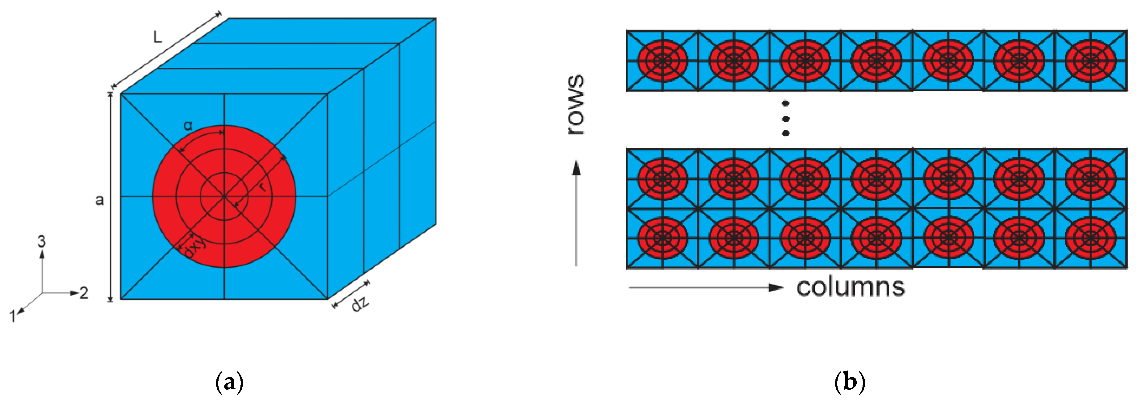
| a (in (mm)) | r ((mm)) | α | dxy (in (mm)) | dz (in (mm)) |
|---|---|---|---|---|
| 0.0077 (0.196) | 0.0033 (0.0846) | 22.5 | 0.0017 (0.0422) | 0.0012 (0.0305) |
| Material Model | Parameter | Remarks | Calibrated Value |
|---|---|---|---|
| MAT_187 (Matrix) | RBCFAC | Ratio of yield stress in equibiaxial compression to yield stress under pure compression. | 0.95 |
| NUEP | Plastic Poisson’s ratio (νp). Defines relationship between transverse and longitudinal plastic strains. | 0.275 | |
| LCID-B | Input stress-plastic strain curve defining yield behavior under equibiaxial tension. | Taken as 80% of the stress-plastic strain response in uniaxial tension | |
| EPFAIL | Equivalent plastic strain value at onset of failure from uniaxial tension test. | 0.0065 | |
| LCID-TRI | Curve that defines equivalent plastic failure strain () as a function of triaxiality. Ordinate values normalized based on value of EPFAIL. | Data shown in Table 5 | |
| MAT_213 (Fiber) | Young’s modulus of orthotropic fiber under longitudinal uniaxial compressive stress. | 31 (10)6 psi (213.7 GPa) | |
| Failure strain of the orthotropic fiber in 1-direction compression. | 0.0156 | ||
| Failure strain of the orthotropic fiber in 1-direction tension. | 0.0065 |
| Condition | Equivalent Plastic Strain at Failure | ||
|---|---|---|---|
| Minimum Triaxiality | −0.890 | 0.0040 | 0.615 |
| Uniaxial Tension | −0.333 | 0.0065 | 1.000 |
| Iosipescu Shear | 0.000 | 0.0350 | 5.385 |
| Uniaxial Compression | 0.333 | 0.0875 | 13.46 |
| Maximum Triaxiality | 0.890 | 0.2100 | 32.31 |
Publisher’s Note: MDPI stays neutral with regard to jurisdictional claims in published maps and institutional affiliations. |
© 2021 by the authors. Licensee MDPI, Basel, Switzerland. This article is an open access article distributed under the terms and conditions of the Creative Commons Attribution (CC BY) license (https://creativecommons.org/licenses/by/4.0/).
Share and Cite
Khaled, B.; Shyamsunder, L.; Robbins, J.; Parakhiya, Y.; Rajan, S.D. Framework for Predicting Failure in Polymeric Unidirectional Composites through Combined Experimental and Computational Mesoscale Modeling Techniques. Fibers 2021, 9, 50. https://0-doi-org.brum.beds.ac.uk/10.3390/fib9080050
Khaled B, Shyamsunder L, Robbins J, Parakhiya Y, Rajan SD. Framework for Predicting Failure in Polymeric Unidirectional Composites through Combined Experimental and Computational Mesoscale Modeling Techniques. Fibers. 2021; 9(8):50. https://0-doi-org.brum.beds.ac.uk/10.3390/fib9080050
Chicago/Turabian StyleKhaled, Bilal, Loukham Shyamsunder, Josh Robbins, Yatin Parakhiya, and Subramaniam D. Rajan. 2021. "Framework for Predicting Failure in Polymeric Unidirectional Composites through Combined Experimental and Computational Mesoscale Modeling Techniques" Fibers 9, no. 8: 50. https://0-doi-org.brum.beds.ac.uk/10.3390/fib9080050