A Hybrid Radix-4 and Approximate Logarithmic Multiplier for Energy Efficient Image Processing

Abstract

Multiplication is an essential image processing operation commonly implemented in hardware DSP cores. To improve DSP cores’ area, speed, or energy efficiency, we can approximate multiplication. We present an approximate multiplier that generates two partial products using hybrid radix-4 and logarithmic encoding of the input operands. It uses the exact radix-4 encoding to generate the partial product from the three most significant bits and the logarithmic approximation with mantissa trimming to approximate the partial product from the remaining least-significant bits. The proposed multiplier fills the gap between highly accurate approximate non-logarithmic multipliers with a complex design and less accurate approximate logarithmic multipliers with a more straightforward design. We evaluated the multiplier’s efficiency in terms of error, energy (power-delay-product) and area utilisation using NanGate 45 nm. The experimental results show that the proposed multiplier exhibits good area utilisation and energy consumption and behaves well in image processing applications.

1. Introduction

Many image processing applications exhibit inherent tolerance on noisy input and small computation error. They might produce an inaccurate but still acceptable output. Pursuing accurate arithmetic operations in these applications can lead to excessive and unnecessary energy consumption. If we introduce an approximation in computation, we can achieve adequate application’s performance with a simpler and energy efficient design.

Approximate computing has emerged as a new paradigm for energy-efficient systems where an acceptable error is induced in computing to achieve more efficient processing [1,2,3,4,5,6]. For example, approximate computing has been used at different system levels [7,8,9,10,11,12,13,14,15,16,17,18] and various approximate arithmetic circuits have been designed to save chip area and energy [8,11,19,20,21,22,23,24,25,26,27,28].

Image and video processing involves many complex operations, which should execute at a high processing rate to suit real-time applications. Hence, these operations are commonly implemented in hardware DSP cores. The results of image and video processing are sounds, images or videos consumed by humans. The small changes in images are often unobservable by humans. For example, lossy compression methods, common in image processing, rely on imperceptible loss of fidelity to substantially reduce image size. Similarly, we anticipate that we can approximate arithmetic operations used in image processing to improve hardware DSP cores’ area, speed, or energy efficiency without substantial loss of fidelity. Multiplication is an essential image processing operation. As multipliers are large circuits that consume a lot of energy, image processing circuits can significantly benefit in terms of power and area consumption by replacing the exact multiplier with an approximate one. In approximate multipliers design, we balance accuracy and energy efficiency such that the multiplier suits the application’s needs.

Most approximate multipliers follow one of the two approaches: approximate logarithmic and approximate non-logarithmic multiplication. Approximate logarithmic multipliers rely on the addition of approximate operands’ logarithms, while approximate non-logarithmic multipliers focus on simplifications in partial product generation and addition. Approximate logarithmic multipliers deliver a more straightforward design but exhibit significantly higher computational error, while approximate non-logarithmic multipliers have a lower computational error at the price of higher design complexity [29,30]. Based on the comparison results for several applications, the authors of [30] suggested that logarithmic multipliers are the best choice for applications that tolerate a significant error but require a small power consumption. On the contrary, they advised using approximate non-logarithmic multipliers in applications requiring better accuracy and allowing a larger power consumption. It has been shown that the approximate logarithmic multipliers behave well in deep-learning accelerators [31,32,33,34,35,36] but can induce a significant error in image processing applications where approximate non-logarithmic multipliers are better choice [37,38,39,40,41,42,43,44].

To reduce energy consumption and keep the error acceptable for image processing applications, we propose encoding the most significant bits with the radix-4 scheme and approximating the least significant bits in the product with an energy-efficient logarithmic multiplier that includes mantissa trimming. We anticipate that the proposed multiplier could achieve similar results in image processing as non-logarithmic multipliers with significantly lower energy consumption. Our goal when designing the proposed multiplier is to use it as a general building block in a DSP application specific integrated circuit design.

In the remainder of the paper, we first review the related work in the field of approximate multipliers. In Section 3, we describe the architecture of the proposed multiplier, which we analyse in terms of synthesis results, error and applicability in image processing applications in Section 4. In Section 5, we conclude the paper with the main findings.

2. Related Work

Mitchell introduced unsigned logarithmic product approximation [45]. His algorithm approximates the logarithm of a binary number and replaces multiplication with addition of logarithms. As Mitchell’s multiplier always underestimates the actual product, Liu et al. [30] proposed the unsigned ALM–SOA multiplier that uses a set-one-adder (SOA) to overestimate the sum of logarithms; hence, it compensates negative errors. Kim et al. [32] proposed a signed logarithmic multiplier that approximates two’s complement with one’s complement, as was previously proposed in [31]. They also proposed the mantissa truncation; their Mitchell–trunck-C1 multiplier keeps only k upper bits of mantissa. Yin et al. [46] proposed unsigned and signed designs of a dynamic range approximate logarithmic multiplier (DR-ALM). The DR-ALM multiplier dynamically truncates input operands and sets the least significant bit of the truncated operand to ‘1’ to compensate for negative errors. Ansari et al. [35] proposed an unsigned logarithmic multiplier with approximate adder (ILM–AA) in the antilogarithm step. They used a near-one-detector to round both operands to their nearest powers of two and the modified SOAk adder, which leads to a double-sided error distribution. Recently, Pilipović et al. [29] proposed an approximate logarithmic multiplier with two-stage operand trimming (TL), which trims the least significant parts of input operands in the first stage and the mantissas of the obtained operands’ approximations in the second stage. The experimental results show that the proposed multiplier exhibits smaller area utilisation and energy consumption than the state-of-the-art logarithmic multipliers with the price of a high error.

The non-logarithmic approximate multipliers commonly simplify the Booth algorithm. Liu et al. [37] proposed approximate Booth multipliers based on radix-4 approximate Booth encoding (R4ABM-k) algorithms. The main idea is to generate k least significant bits of partial products with approximate radix-4 encoding, while the most-significant bits are generated exactly. Zendegani et al. [38] proposed the approximate signed rounding based multiplier (AS–ROBA) that rounds the operands to the nearest exponent of two. The proposed multiplier has higher accuracy than logarithmic multipliers, and the experiments in image smoothing and sharpening revealed the same image qualities as those of exact multiplication algorithms. The RAD$2^k$ multiplier [39] employs a hybrid encoding technique, where the n-bit input operand is divided into two groups: the upper part of $n-k$ bits and the lower part of k bits. The upper part is exactly encoded using the radix-4 encoding, while the lower part is approximately encoded with the radix-$2^k$ encoding. The approximations round the radix-$2^k$ values to their nearest power of two. The HLR–BM multiplier [47] addresses the issue of generating multiples of the $\pm 3$ multiplicand in the radix-8 Booth encoding. It approximates the $\pm 3$ multiplicands to their nearest power of two, such that the errors complement each other. Similar to RAD$2^k$ [39], the authors employed the hybrid radix encoding.

Pilipović et al. [33] were the first to propose a hybrid-encoding logarithmic multiplier (LOBO) that uses the logarithmic approximation to generate the least significant part of the product and the radix-4 Booth encoding to compute the most significant part of the product.

Table 1. Overview of the state-of-the-art 16-bit approximate multipliers [29].

Multiplier	Group	Energy (fJ)	NMED $(·{10}^{-3})$
Mitchell [45]		57.70	9.27
ALM–SOA11 [30]		53.95	8.06
Mitchell–trunc8-C1 [32]	logarithmic	50.05	10.56
DR–ALM5 [46]		42.80	5.27
ILM–AA [35]		41.98	7.20
TL16–8/4 [29]		28.70	11.84
HLR–BM2 [47]		107.18	0.01
R4ABM2–20 [37]	non-logarithmic	93.80	0.41
RAD1024 [39]		61.50	0.44

, taken from Pilipović et al. [29], summarises some of the state-of-the-art approximate multipliers in terms of energy and normalised mean error distance (NMED). The upper part contains six approximate logarithmic multipliers, while the bottom part contains three approximate non-logarithmic multipliers. Table 1 confirms the claims in [29,30] that approximate logarithmic multipliers have smaller energy consumption than approximate non-logarithmic multipliers at the price of a higher error.

3. The Hybrid Radix-4 and Approximate Logarithmic Multiplier

With the hybrid radix-4 and approximate logarithmic multiplier (HRALM), we try to combine radix-4 encoding to deliver small computational error and logarithmic product approximation to get low power consumption and area utilisation. We select the radix-4 algorithm as it is a powerful method to improve the performance of multiplication. It reduces the number of partial products by half by using the radix-4 recoding technique, where we consider the bits in groups of three such that each group overlaps the previous one by one bit [48]. To multiply 16-bit integers X and Y, we split the integer X into two parts and keep Y unchanged. This way, instead of generating eight partial products with exact radix-4 encoding, we reduce the number of partial products to two only.

The value of the integer X in two’s complement equals

$$\begin{array}{c}\hfill X=-X_{15}·2^{15}+\sum _{i=0}^{14}{X}_i·2^i,\end{array}$$

(1)

where $X_i$ represents its ith bit. Following the idea proposed by Pilipović and Bulić [33], we encode the three most significant bits using radix-4 encoding and keep the rest in binary encoding,

$$\begin{array}{c}\hfill X=X_R·2^{14}+X_L,\end{array}$$

(2)

with

$$X_R=-2·X_{15}+X_{14}+X_{13}\mathrm{and}$$

(3)

$$X_L=-X_{13}·2^{13}+\sum _{i=0}^{12}{X}_i·2^i.$$

(4)

The value $X_R$ is obtained from the group of three most significant bits using radix-4 encoding. It can take only values $0,\pm 1,\pm 2$. In such a way, the most significant partial product is obtained by simple operations, e.g., shifting and inversion of the operand Y, avoiding the generation of odd multiples such as $\pm 3·Y$. The term $X_{13}$ in (3) contributes $X_{13}·2^{14}=2·X_{13}·2^{13}$ to (2), therefore we subtract $X_{13}·2^{13}$ in (4) to form the correct value of X. Note that $X_L$ is a value of a 14-bit integer given in two’s complement.

Taking into account (2), we can write the exact product as

$$P=X·Y=P{P}_R·2^{14}+P{P}_L,$$

(5)

where $P{P}_R=X_R·Y$ and $P{P}_L=X_L·Y$ represent two partial products. The partial product $P{P}_R$ is nonzero for large absolute values, $|X|\ge 2^{13}$. Therefore, to keep the product approximation close to the exact value, we generate the partial product $P{P}_R$ using the exact radix-4 partial product generator [39]. On the contrary, we apply an approximate signed logarithmic multiplier to get the estimate ${\widetilde{PP}}_L$ of the partial product $P{P}_L$.

Figure 1 presents the architecture of the HRALM multiplier. Firstly, we split the integer X into two parts, $X_R$ and $X_L$. In the left branch, the radix-4 partial product generator takes the 3-bit $X_R$ and the 16-bit integer Y to output the 17-bit partial product $P{P}_R$ and the signal $neg$ that determines the sign of $X_R$. In the right branch, the signed approximate logarithmic multiplier takes the 14-bit integer $X_L$ and the 16-bit integer Y to output the 30-bit approximate partial product ${\widetilde{PP}}_L$. The final product approximation $\tilde{P}$ is a 32-bit integer, formed by fusing the partial product $P{P}_R$ and the signal $neg$ from the left branch and the approximate partial product ${\widetilde{PP}}_L$ from the right branch.

3.1. Exact Radix-4-Based Multiplier

The exact radix-4-based multiplier in Figure 2 comprises a radix-4 encoder and 17 parallely connected partial product generation (PPG) units.

Each PPG unit outputs one bit of the partial product in accordance to the signals $one$, $two$ and $neg$ from the radix-4 encoder. The radix-4 encoder sets $one$ when $|X_R|=1$, $two$ when $|X_R|=2$ and $neg$ when $X_R$ is negative, i.e.,

$$\begin{array}{c}neg=\mathrm{sign}\left(X_R\right)=\left\{\begin{array}{cc}1;\hfill & X_R<0\\ 0;\hfill & \mathrm{otherwise}\end{array}\right..\hfill \end{array}$$

(6)

If the signal $neg$ equals zero, the ${\mathrm{PPG}}_i$ unit outputs zero when the control signals $one$ and $two$ are zero; $Y_i$ when $one$ is set; and $Y_{i-1}$ when $two$ is set, to accommodate for multiplication by 0, 1 and 2, respectively. If the signal $neg$ equals one, the unit inverts the above output bits. In the case of bit inversion, we get one’s complement of the 17-bit partial product $P{P}_R$. For two’s complement, we must add $neg$ to the result; to reduce the number of adders, we postpone this operation to the partial products fuser.

3.2. Approximate Logarithmic Multiplier

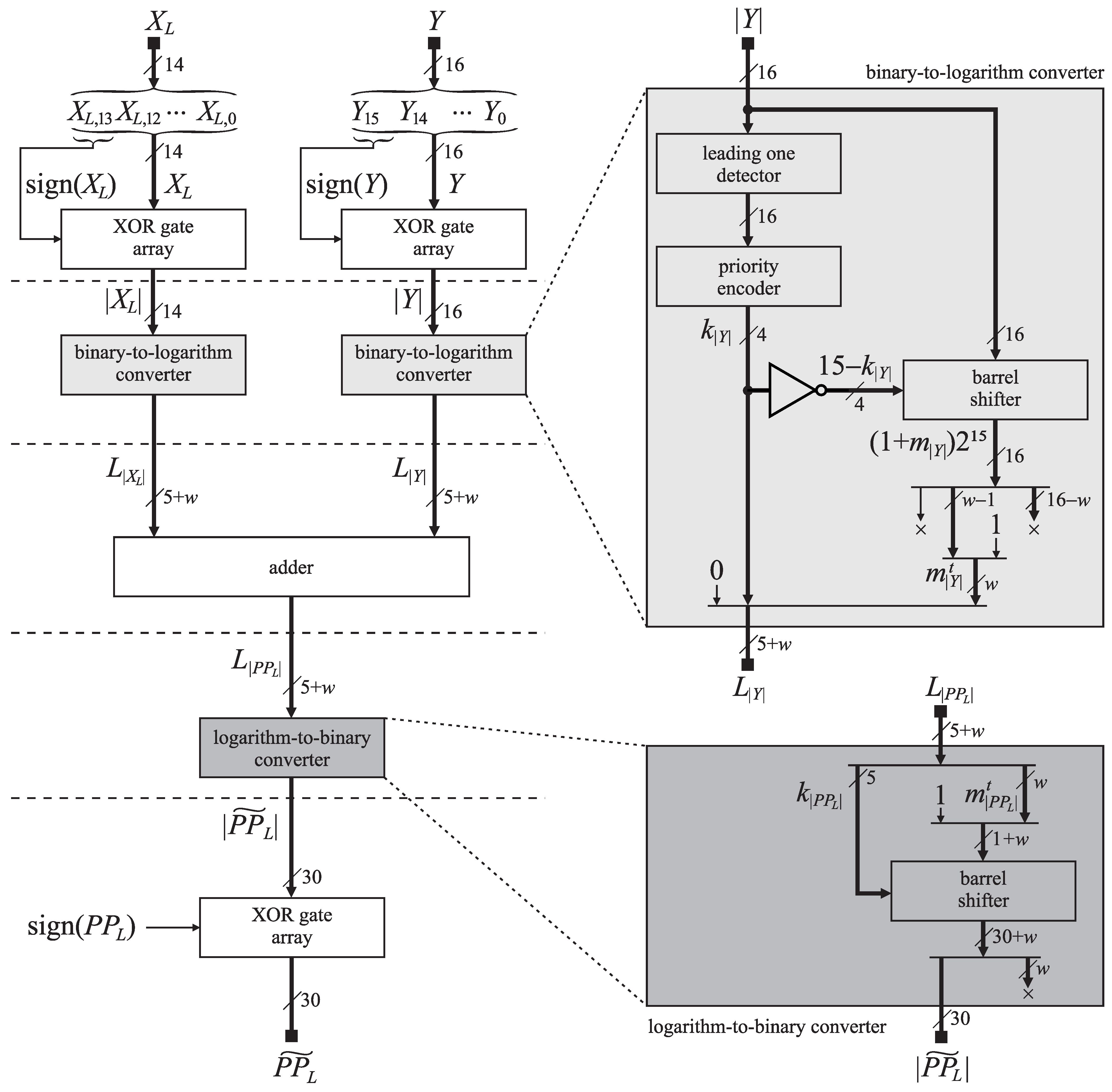
The signed approximate logarithmic multiplier presented in Figure 3 comprises two sign conversion stages and three intermediate stages: the binary-to-logarithm conversion of operands, the addition of their logarithms and the logarithm-to-binary conversion of the sum.

3.2.1. Sign Operations

The logarithm conversion works only on positive integers; therefore, we first take out the operands’ $X_L$ and Y signs, $\mathrm{sign}\left(X_L\right)$ and $\mathrm{sign}\left(Y\right)$, and continue with approximation of their absolute values in one’s complement, $|X_L|$ and $|Y|$. In the end, we consider the sign of the resulting partial product,

$$\begin{array}{c}\hfill {\widetilde{PP}}_L=\mathrm{sign}\left(P{P}_L\right)·|{\widetilde{PP}}_L|=\mathrm{sign}\left(X_L\right)·\mathrm{sign}\left(Y\right)·|{\widetilde{PP}}_L|.\end{array}$$

(7)

In one’s complement, the most significant bit of an integer represents the sign. Hence, to get the absolute value in the first stage, we need an array of XOR gates to invert each bit of an integer when the sign is set. Using another array of XOR gates, we also put the correct sign to the partial product ${\widetilde{PP}}_L$ in the last stage.

3.2.2. The Binary-to-Logarithm Conversion Stage

The binary-to-logarithm conversion stage outputs the input operands’ logarithms. As the operand $X_L$ and Y differ only in bit-width, we limit the description to the operand Y only. We can write its absolute value as

$$\begin{array}{c}\hfill |Y|=2^{k_{|Y|}}·(1+m_{|Y|}),\end{array}$$

(8)

where $k_{|Y|}=\lfloor {log}_2|Y|\rfloor$ denotes the position of the leading one bit and

$$m_{|Y|}=2^{-k_{|Y|}}\sum _{i=0}^{k_{|Y|}-1}{|Y|}_i{2}^i=\sum _{i=0}^{k_{|Y|}-1}{|Y|}_i{2}^{-k_{|Y|}+i}$$

(9)

is the logarithm mantissa bounded to interval $[0,1)$. The logarithm of $|Y|$ then becomes

$${log}_2|Y|=k_{|Y|}+{log}_2(1+m_{|Y|}).$$

(10)

To avoid the complex computation of the second term, Mitchell [45] proposed replacing it with a piecewise linear approximation, ${log}_2(1+m_{|Y|})\approx m_{|Y|}$. Inside an interval with the constant exponent $k_{|Y|}$, the approximation equals the exact value when $m_{|Y|}=0$ and underestimates it when $0<m_{|Y|}<1$. To make the design smaller, we keep only w most significant bits of the mantissa. By setting the least significant bit of the trimmed mantissa

$$m_{|Y|}^t=\sum _{i=k_{|Y|}-(w-1)}^{k_{|Y|}-1}{|Y|}_i{2}^{-k_{|Y|}+i}+2^{-w}$$

(11)

we provide a mean value approximation of the removed bits. Introducing both approximations to (10), we get

$${log}_2|Y|\approx k_{|Y|}+m_{|Y|}^t=L_{|Y|},$$

(12)

with $L_{|Y|}$ denoting the approximation of ${log}_2|Y|$.

The upper detail in Figure 3 illustrates the binary-to-logarithm converter. We use the leading-one detector and the priority encoder to obtain the 4-bit exponent $k_{|Y|}$. The barrel shifter aligns $|Y|$ for further processing by shifting it $15-k_{|Y|}$ bits left. We ignore the most significant bit (leading one bit) and the $16-w$ least significant bits. The remaining bits represent the $w-1$ most significant bits of the mantissa $m_{|Y|}$ to which we append ‘1’ to form the trimmed mantissa $m_{|Y|}^t$. In (12), the exponent $k_{|Y|}$ is an unsigned integer and the mantissa $m_{|Y|}^t$ is bounded to the interval $[0,1)$ assuring that there is no carry from mantisa. Therefore, in the hardware implementation, we can avoid summation in (12) by simply appending bits ${|Y|}_{k_{|Y|}-1},\dots ,{|Y|}_{k_{|Y|}-w}$ of the mantissa $m_{|Y|}^t$ to the bits of the exponent $k_{|Y|}$. Additionally, we prepend ’0’ to the integer exponent $k_{|Y|}$. Hence, the logarithm approximation $L_{|Y|}$ has $5+w$ bits that are required by the adder in the next stage.

3.2.3. The Addition of Logarithms and the Antilogarithm Conversion

The addition stage outputs the approximate logarithm of the partial product

$$L_{|P{P}_L|}=L_{|X_L|}+L_{|Y|}=k_{|X_L|}+m_{|X_L|}^t+k_{|Y|}+m_{|Y|}^t=k_{|P{P}_L|}+m_{|P{P}_L|}^t,$$

(13)

where the five most significant bits form the integer exponent $k_{|P{P}_L|}$ and the w least significant bits form the fractional mantissa $m_{|P{P}_L|}$. Following the equation

$$|{\widetilde{PP}}_L|=(1+m_{|P{P}_L|}^t)·2^{k_{|P{P}_L|}},$$

(14)

the antilogarithm stage outputs the absolute value of the approximate partial product.

The lower detail in Figure 3 shows the logarithm-to-binary converter. We split the logarithm approximation $L_{|P{P}_L|}$ into two parts: the five most significant bits form the exponent $k_{|P{P}_L|}$, while the w least significant bits form the mantissa $m_{|P{P}_L|}^t$. By appending ‘1’ to the most significant position of the mantissa, we get $1+m_{|P{P}_L|}^t$, which we shift $k_{|P{P}_L|}$ bits left following (14). The 30 most significant bits of the result form the integer part of $|{\widetilde{PP}}_L|$, which we drive to the partial products fuser.

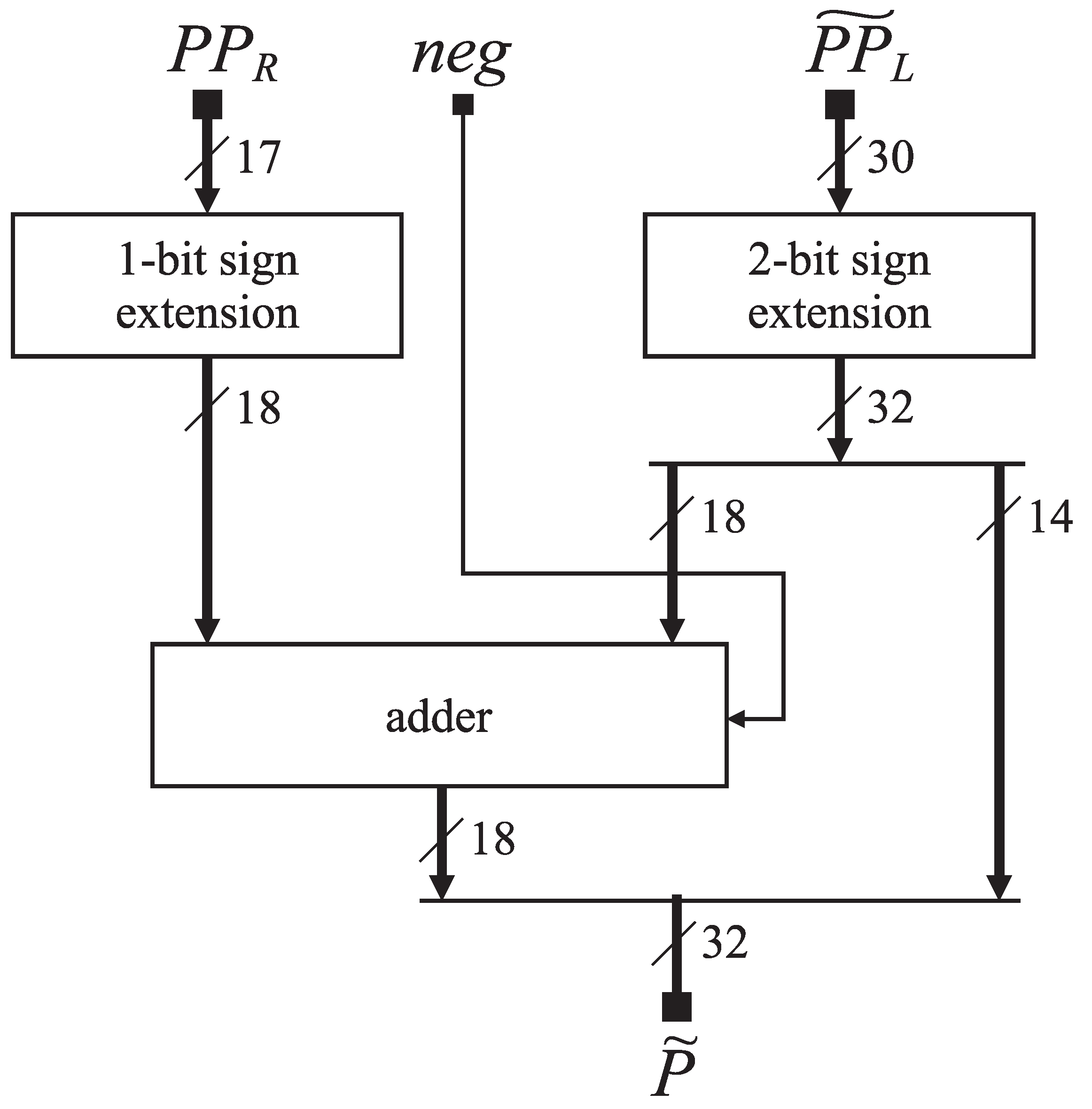
3.3. Partial Products Fuser

The partial products fuser generates the approximation of the final product (5) by considering the results of the exact radix-4 based multiplier, and the approximate logarithmic multiplier

$$\begin{array}{c}\hfill \tilde{P}=P{P}_R·2^{14}+\widetilde{P{P}_L}.\end{array}$$

(15)

Figure 4 shows the partial products fuser. Firstly, we sign-extend both partial products by appending one or two most significant bits. The 14 least significant bits of the first term in (15) are zero, so we can use only an 18-bit adder. Therefore, we split ${\widetilde{PP}}_L$ into two parts and drive its 18 most significant bits to the adder. We also drive the signal $neg$ from the exact radix-4 multiplier as the input carry to form the two’s complement representation of the $P{P}_R$. Finally, we concatenate 18 bits of the sum and 14 least significant bits of ${\widetilde{PP}}_L$ to get the final product approximation $\tilde{P}$.

4. Results and Discussion

To evaluate the HRALM multiplier, we performed a comparative study with several recently published 16-bit state-of-the-art multipliers regarding hardware characteristics and image processing applicability. We compared the proposed multiplier with the 16-bit approximate logarithmic multipliers Mitchell–trunc8-C1 [32], ALM–SOA11 [30], DR–ALM5 [46], ILM–AA [35], TL16–8/4 [29] and AS–ROBA [38]; the approximate non-logarithmic multipliers RAD1024 [39] and HLR–BM2 [47]; and the hybrid LOBO12–12/8 [33] multiplier. For each proposed multiplier design, we selected its parameters such that it delivers acceptable error and energy consumption. The multipliers in [30,35] are unsigned, while the multipliers in [29,32,33,38,39,46,47] are signed. We extended the unsigned ALM–SOA11 and ILM–AA multipliers to signed in the same way as the approximate logarithmic multiplier of our design.

4.1. Synthesis Results

We analysed and compared the hardware performance of the proposed HRALMw multipliers, where w denotes the length of the trimmed mantissa, in terms of power, area, delay, power-delay-product (PDP), the normalised mean error distance (NMED) and the mean relative error distance (MRED). The multipliers were implemented in Verilog and synthesised to 45 nm Nangate Open Cell Library. We used timing with a 10 MHz virtual clock, a 5% signal toggle rate and output load capacitance of 10 fF to evaluate the power.

As illustrated in Figure 5a, delay, area and power are reported from the ASIC design flow. We implemented all multipliers in this study in Verilog and synthesised them using OpenROAD Design Flow [49]. Besides, we implemented the multipliers in Python to simulate all operand pairs’ products and assess the error. We compared all products from the exact multiplier and an approximate multiplier to report the error metrics (Figure 5b).

Table 2. The synthesis results, NMED (normalised mean error distance) and MRED (mean relative error distance) for 16-bit multipliers.

Multiplier	Delay (ns)	Power (µW)	Area (µm2)	PDP (fJ)	NMED (·10−3)	MRED (%)
Exact radix-4	1.74	69.20	1576.58	120.41	0	0
HRALM4	1.75	34.00	878.60	59.50	2.94	2.09
HRALM3	1.70	32.40	842.42	55.08	4.28	2.98
HRALM2	1.60	30.70	815.29	49.12	7.54	5.20
Mitchell–trunc8-C1 [32]	1.43	35.00	910.25	50.05	10.56	3.46
ALM–SOA11 * [30]	1.47	36.70	952.01	53.95	8.06	3.33
DR–ALM5 [46]	1.31	32.70	831.78	42.80	5.27	4.32
ILM–AA * [35]	1.51	27.80	780.18	41.98	7.20	2.90
TL16–8/4 [29]	1.13	25.40	702.24	28.70	11.84	3.94
AS–ROBA [38]	1.88	69.30	1621.80	130.30	6.90	2.93
HLR–BM2 [47]	1.76	60.90	1312.18	107.18	0.01	0.02
RAD1024 [39]	1.50	41.00	1008.67	61.50	0.44	0.96
LOBO12–12/8 [33]	1.71	36.10	904.93	61.73	1.85	2.17

* converted to signed.

shows the synthesis results and error metrics for all multipliers.

The parameter w affects the size of the HRALM multiplier. A smaller w leads to a simpler logarithm and antilogarithm conversion, resulting in smaller delay, area utilisation and PDP, but it increases NMED. The HRALM multipliers utilise from 52% to 56% of the area and consume only 41–49% of the energy required in the exact radix-4 multiplier. On the one hand, the HRALM3 multiplier outperforms all non-logarithmic multipliers in terms of area and PDP at the expense of a larger NMED. The PDP of the HRALM3 multiplier is 89% of the RAD1042 multiplier’s PDP, while its NMED and MRED are 9.7 and 3.1 times higher, respectively. On the other hand, the HRALM3 multiplier possesses a smaller NMED but delivers a larger area and PDP compared to the logarithmic multipliers. The error measures NMED and MRED of the HRALM3 multiplier are only 81% and 69% of the values provided by DR–ALM5 multiplier, respectively, while its PDP is 29% higher. The HRALM2 multiplier delivers similar performance as the logarithmic multipliers in all aspects, while the HRALM4 delivers similar hardware performance as the non-logarithmic multipliers and LOBO12–12/8 [33].

Figure 6 illustrates the scatter plot that displays values for NMED, PDP of the studied multipliers. If the rectangle with the coordinate origin and the multiplier at its edges is empty (e.g., RAD1024), no multiplier with smaller error and energy consumption exists. Otherwise, at least one multiplier outperforms the selected one (e.g., ILM–AA and DR–ALM5 outperform HRALM2). The RAD1024, HRALM3 and DR–ALM5 multipliers have empty rectangles; hence, we could consider them potentially good candidates for an application Although HRALM4 has an empty rectangle, it poses a much higher error with similar hardware performance as RAD1024, making it a better choice than HRALM4. The user would strive to select a multiplier with the smallest energy consumption and still an acceptable error for his application. For image processing, one would select multipliers with small NMED on the left part of the scatter plot. For error-resilient neural network processing, one would choose among energy-efficient multipliers on the right side.

The HRALM3 multiplier fills the gap between the approximate non-logarithmic multipliers and the approximate logarithmic multipliers and becomes our design of choice for further analyses. We anticipate that the proposed HRALM3 multiplier, with slightly higher energy consumption but lower NMED than non-logarithmic multipliers, behaves well and can replace non-logarithmic multipliers in many image processing applications.

4.2. Application Case Studies

To show the HRALM3 multiplier’s applicability, we evaluated the multipliers in image processing applications. To cover a range of applications in image processing as comprehensive as possible, we selected the following test cases: (i) image smoothing, where small integer numbers appear in the smoothing kernel to evaluate how multipliers behave when multiplying pixel values with small numbers; (ii) image multiplication, where the full range of values is present in the image and mask; and (iii) lossy image compression with a large number of multiplications per image block.

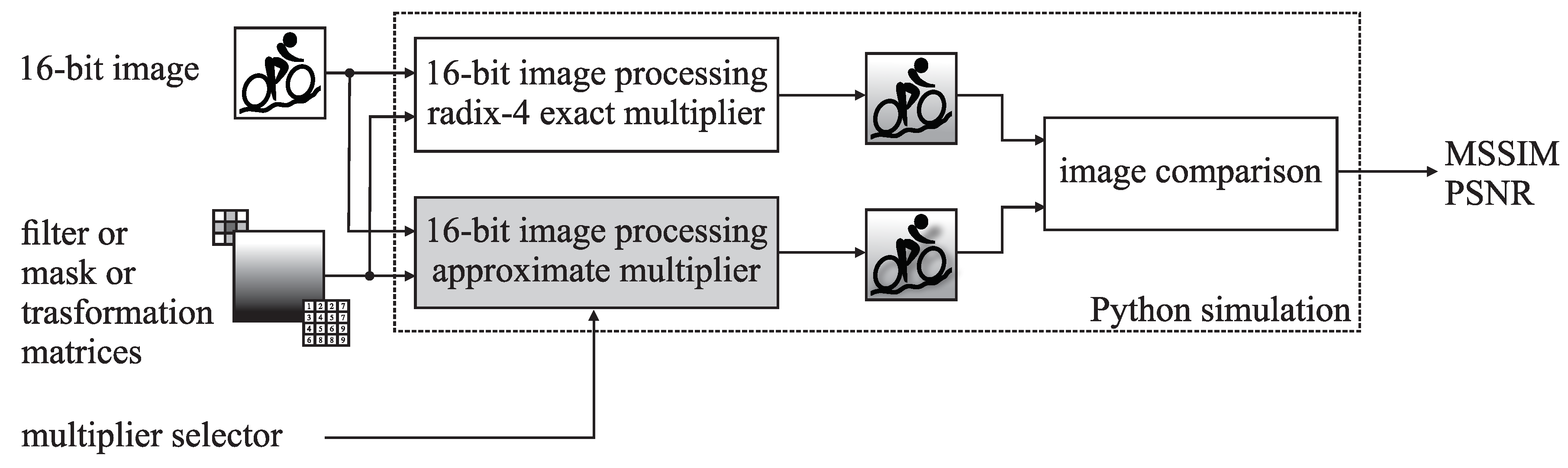
Figure 7 illustrates the workflow for multiplier evaluation in image processing. We implemented the image processing applications in Python, where we replaced the multiplication operator with our routines that implement various approximate multiplier designs. All images were processed with the exact multiplier and approximate multipliers to assess the performance. For evaluation, we used the mean structural similarity index (MSSIM) [50] and the peak-signal-to-noise ratio (PSNR). Besides, we include a set of images after each application case study to visually compare the image quality obtained by the exact radix-4 multiplier, the HRALM3 multiplier and two multipliers with similar performance as HRALM3: RAD1024 and DR–ALM5.

We ran the tests on six 16-bit grayscale images from TESTIMAGES database [51]: building, cards, flowers, roof, snail and wood game. We uniformly shifted the pixels in an input image from $[0,2^{16})$ to $[-2^{15},2^{15})$ to adapt for signed 16-bit multiplication. We uploaded the Supplementary Materials containing the images obtained with all multipliers to [52].

4.2.1. Image Smoothing

Image smoothing reduces noise and details in the image [53] by convolving the image with the smoothing kernel

$$K_S=\frac{1}{256}\left[\begin{array}{ccc}21& 31& 21\\ 31& 48& 31\\ 21& 31& 21\end{array}\right].$$

(16)

We implemented the division by 256 by trimming the 8 least significant bits of the convolution sum.

Table 3. The MSSIM and PSNR metrics in the image smoothing application.

	Building		Cards		Flowers		Roof		Snails		Wood Game
	MSSIM	PSNR (dB)	MSSIM	PSNR (dB)	MSSIM	PSNR (dB)	MSSIM	PSNR (dB)	MSSIM	PSNR (dB)	MSSIM	PSNR (dB)
HRALM3	1.00	41.15	1.00	41.27	1.00	41.41	1.00	41.37	1.00	41.34	1.00	41.28
Mitchell–trunc8-C1 [32]	0.99	37.55	1.00	36.53	0.99	37.91	0.99	36.89	0.99	37.91	1.00	37.64
ALM–SOA11 [30]	0.99	39.56	0.99	39.17	0.99	39.78	0.99	39.31	0.99	39.78	0.99	39.45
DR–ALM5 [46]	0.97	37.92	0.98	38.49	0.98	38.56	0.99	37.35	0.97	38.21	0.98	37.80
ILM–AA [35]	0.99	39.75	1.00	39.24	0.99	40.08	1.00	40.00	0.99	40.08	1.00	40.04
TL16–8/4 [29]	0.98	37.44	0.98	36.55	0.99	38.02	0.99	36.22	0.98	37.52	0.98	36.35
AS–ROBA [38]	1.00	41.50	1.00	41.45	1.00	41.30	1.00	41.37	1.00	41.53	1.00	41.67
HLR–BM2 [47]	1.00	54.62	1.00	53.06	1.00	56.38	1.00	56.45	1.00	54.54	1.00	51.19
RAD1024 [39]	1.00	41.66	1.00	41.67	1.00	41.67	1.00	41.67	1.00	41.66	1.00	41.67
LOBO12–12/8 [33]	0.99	40.69	0.99	40.42	0.99	40.99	1.00	42.55	0.99	40.67	0.99	40.38

reports the PSNR and MSSIM for image smoothing. Overall, the HRALM3 multiplier exhibits high PSNR and MSSIM for image smoothing, which indicates that it can replace the exact multiplier without a significant decrease in image quality. It delivers better PSNR and MSSIM than other state-of-the-art logarithmic approximate multipliers due to its better error characteristic. Moreover, HRALM3 delivers similar PSNR and MSSIM as highly accurate approximate non-logarithmic multipliers but with significantly lower energy consumption, as shown in Table 2.

Figure 8 visualises wood game image smoothing for selected multipliers. The most obvious difference is in a continuous gradation of grey tone in the image background—more pronounced posterisation (banding) can be observed in the images with lower MSSIM and PSNR.

4.2.2. Image Multiplication

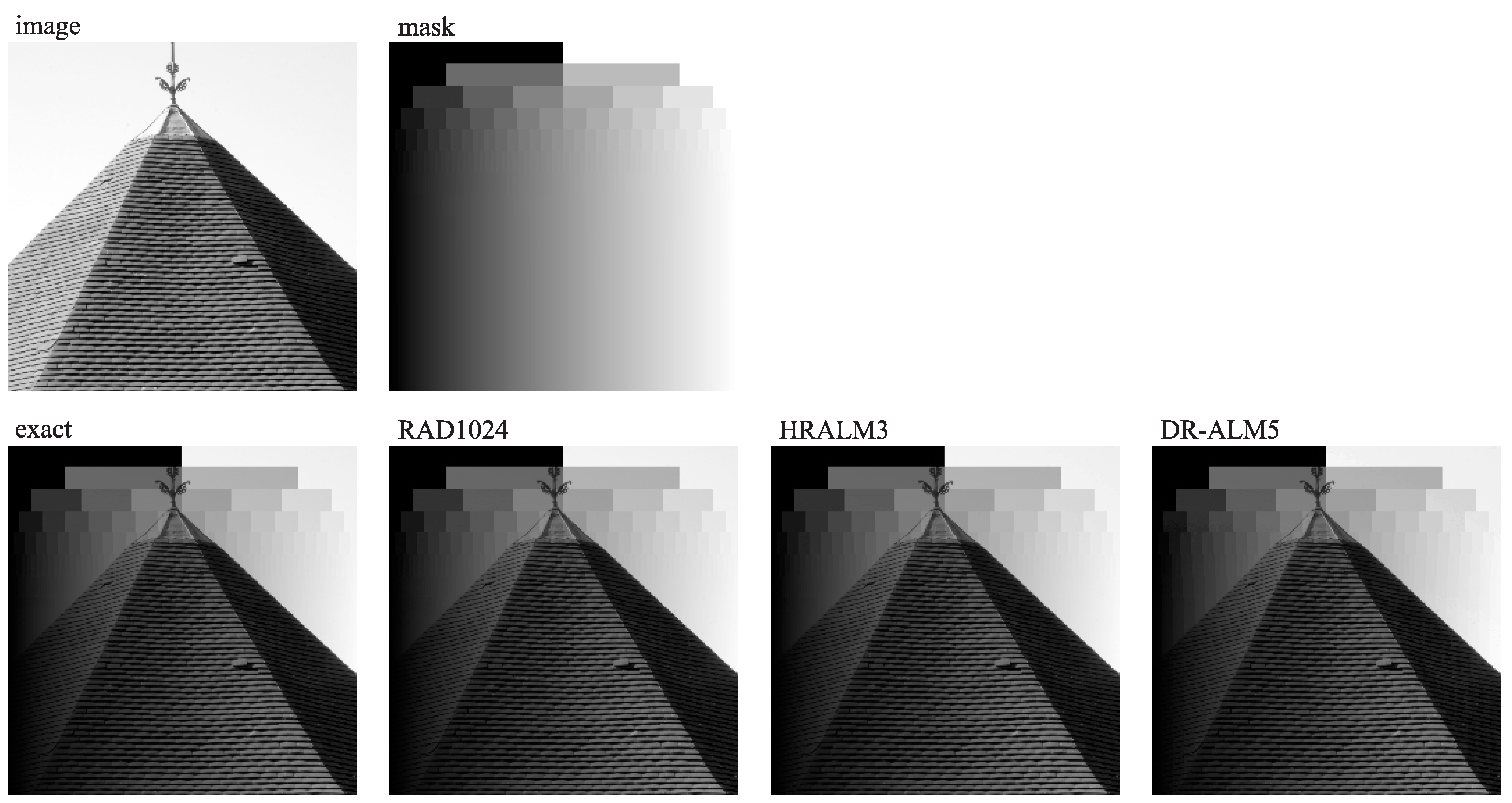
In image multiplication, we perform a pixel-by-pixel multiplication between an input image and a mask. The product determines the value of the corresponding pixel in the output image.

Table 4. The MSSIM and PSNR metrics for image multiplication.

	Building		Cards		Flowers		Roof		Snails		Wood Game
	MSSIM	PSNR (dB)	MSSIM	PSNR (dB)	MSSIM	PSNR (dB)	MSSIM	PSNR (dB)	MSSIM	PSNR (dB)	MSSIM	PSNR (dB)
HRALM3	1.00	52.93	1.00	54.91	1.00	54.07	1.00	55.48	1.00	55.03	1.00	57.42
Mitchell–trunc8-C1 [32]	0.98	38.52	0.99	37.74	0.98	42.47	0.99	39.02	0.98	34.82	0.96	30.02
ALM–SOA11 [30]	0.99	49.66	1.00	48.11	0.99	49.49	1.00	49.69	1.00	50.31	1.00	50.72
DR–ALM5 [46]	0.99	49.50	0.99	47.02	0.99	48.91	0.99	47.94	0.99	48.90	0.99	47.88
ILM–AA [35]	0.99	50.76	1.00	49.23	0.99	50.75	1.00	51.30	1.00	51.62	1.00	52.43
TL16–8/4 [29]	0.98	45.66	0.98	44.16	0.98	45.75	0.98	44.56	0.99	46.02	0.97	45.17
AS–ROBA [38]	0.99	50.69	1.00	49.37	0.99	50.87	1.00	51.74	1.00	51.62	1.00	52.68
HLR–BM2 [47]	1.00	58.71	1.00	57.31	1.00	58.22	1.00	58.64	1.00	58.63	1.00	57.97
RAD1024 [39]	1.00	71.66	1.00	71.52	1.00	71.55	1.00	71.56	1.00	71.60	1.00	71.46
LOBO12–12/8 [33]	1.00	61.37	1.00	59.64	1.00	61.00	1.00	61.76	1.00	61.56	1.00	61.70

reports the PSNR and MSSIM for 16-bit image multiplication. HRALM3 exhibits considerably higher PSNR and MSSIM than approximate logarithmic multipliers and delivers similar PSNR and MSSIM as non-logarithmic multipliers with significantly lower energy consumption, as detailed in Table 2.

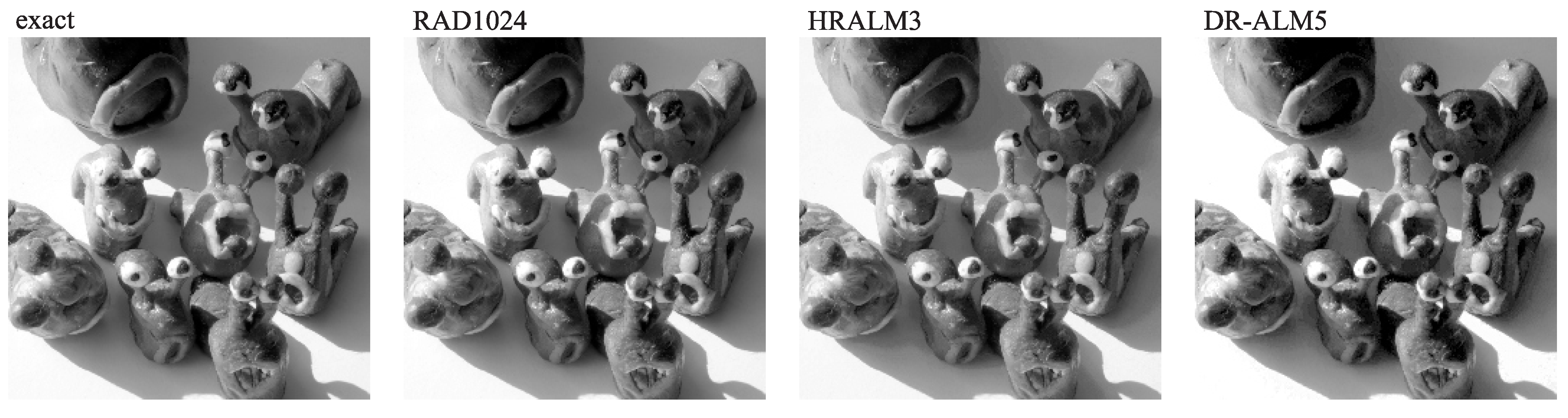
Figure 9 visualises image multiplication in the roof image. In the image multiplication, the image quality more strongly correlates with PSNR. The logarithmic DR–ALM5 multiplier with low PSNR has noticeable posterisation in the sky to the lower right of the roof, where it should not exist. The HRALM3 multiplier, similarly to the non-logarithmic RAD1024 multiplier and the exact multiplier, does not noticeably distort the sky.

4.2.3. Lossy Image Compression

Two-dimensional discrete cosine transform (DCT) is a widely used technique for lossy image compression. DCT transforms the image from the spatial domain to the frequency domain, where the high-frequency DCT coefficients are selectively discarded to allow for efficient compression [54,55].

In the compression stage, we apply DCT to the non-overlapping blocks of 8 × 8 pixels. For the block $\mathbf{B}$, we get the coefficients $\mathbf{D}$, following the matrix multiplication

$$\begin{array}{c}\hfill \mathbf{D}=\mathbf{T}·\mathbf{B}·{\mathbf{T}}^{\mathsf{T}},\end{array}$$

(17)

with the elements of transformation matrix $\mathbf{T}$ being

$$\begin{array}{c}\hfill {\mathbf{T}}_{ij}=\left\{\begin{array}{cc}{2}^{-3/2},\hfill & i=0,0\le j\le 7\hfill \\ 2^{-1}cos\frac{\pi i(2j+1)}{16},\hfill & 0<i\le 7,0\le j\le 7\hfill \end{array}\right..\end{array}$$

(18)

We reduce the amount of information in the high-frequency coefficients by element-wise multiplication of the coefficients $\mathbf{D}$ with the inverse of elements of the 8 × 8 quantisation matrix $\mathbf{Q}\left(F\right)$,

$$\begin{array}{c}\hfill {\mathbf{C}}_{ij}=\mathrm{round}({\mathbf{D}}_{ij}·{\mathbf{Q}}_{ij}^{-1}\left(F\right)).\end{array}$$

(19)

The elements of the quantisation matrix $\mathbf{Q}\left(F\right)$ are determined from the standard luminance quantisation matrix ${\mathrm{Q}}^L$, provided by Independent JPEG Group, and the quality factor F as [56,57]

$$\begin{array}{c}\hfill Q_{ij}\left(F\right)=\left\{\begin{array}{cc}\lfloor (2-F/50)·Q_{ij}^L+0.5\rfloor ,\hfill & 50\le F\le 100\hfill \\ \lfloor 5000/F·Q_{ij}^L+0.5\rfloor ,\hfill & 1\le F<50\hfill \end{array}\right.,\end{array}$$

(20)

where smaller values of the factor F correspond to higher compression ratios and thus poorer image quality.

In the decompression stage, we start with compressed coefficients $\mathbf{C}$, where we first reverse the quantisation

$$\begin{array}{c}\hfill {\mathbf{D}}_{ij}^{*}={\mathbf{C}}_{ij}·{\mathbf{Q}}_{ij}\left(F\right)\end{array}$$

(21)

and then apply the inverse DCT to obtain the reconstructed image block

$$\begin{array}{c}\hfill {\mathbf{B}}^{*}={\mathbf{T}}^{\mathrm{T}}·{\mathbf{D}}^{*}·\mathbf{T}.\end{array}$$

(22)

To use the above equation in fixed-point arithmetic with signed multipliers and retain maximal precision of coefficients in matrix $\mathbf{T}$, we scale them by a factor $2^{16}$ and compensate for the scaling after each multiplication by discarding 16 least significant bits of the product. In the same way, we perform the operations involving the matrix ${\mathbf{Q}}^{-1}\left(F\right)$.

Table 5. The MSSIM and PSNR metrics for lossy image compression for the quality factor $F=50$.

	Building		Cards		Flowers		Roof		Snails		Wood Game
	MSSIM	PSNR (dB)	MSSIM	PSNR (dB)	MSSIM	PSNR (dB)	MSSIM	PSNR (dB)	MSSIM	PSNR (dB)	MSSIM	PSNR (dB)
HRALM3	0.97	38.77	0.98	37.34	0.98	39.23	0.99	39.14	0.97	38.76	0.98	37.42
Mitchell–trunc8-C1 [32]	0.91	33.71	0.92	32.71	0.93	33.74	0.93	32.12	0.91	34.09	0.93	34.74
ALM–SOA11 [30]	0.96	34.26	0.96	31.32	0.97	33.39	0.97	31.85	0.96	33.93	0.96	31.84
DR–ALM5 [46]	0.92	31.62	0.95	28.51	0.91	30.32	0.95	29.46	0.93	30.47	0.95	28.84
ILM–AA [35]	0.95	36.50	0.97	33.21	0.95	35.99	0.98	34.68	0.95	35.29	0.97	32.96
TL16–8/4 [29]	0.94	36.73	0.91	33.88	0.93	34.36	0.95	34.18	0.93	36.79	0.94	35.94
AS–ROBA [38]	0.95	36.50	0.97	33.21	0.95	35.99	0.98	34.68	0.95	35.29	0.97	32.96
HLR–BM2 [47]	0.99	43.36	0.99	40.47	0.99	42.58	0.99	40.96	0.99	42.48	0.99	40.45
RAD1024 [39]	1.00	52.65	1.00	50.61	1.00	51.30	1.00	51.10	1.00	52.20	1.00	51.53
LOBO12–12/8 [33]	0.99	46.40	0.99	43.18	0.99	44.25	0.99	44.76	0.99	46.77	0.99	47.72

and Figure 10 show the qualities of the decompressed images using different multipliers combinations in the compression stage and the exact radix-4 multiplier in the decompression stage. (R2:C3) We use approximate multipliers in the image compression stage Equations (17) and (19) and exact multiplication in the decompression stage Equations (21) and (22).

In the lossy compression, the RAD1024, HLR–BM2 and LOBO multipliers offer the highest PSNR and MSSIM. The proposed HRALM3 multiplier is behind them with a slightly lower PSNR and MSSIM. It is worth pointing out that it also achieves considerable improvements in hardware parameters compared to RAD1024, HLR–BM2 and LOBO, as shown in Table 2. Again, the logarithmic multipliers offer low MSSIM and PSNR and introduce visible artefacts in images.

We also evaluate lossy image compression in terms of quality factor. Figure 11 shows the results of PSNR and MSSIM for the decompressed snails image using four different 16-bit signed multipliers: exact radix-4, RAD1024, HRALM3 and DR–ALM5 in the compression stage and the exact radix-4 multiplier in the decompression stage. We evaluated PSNR and MSSIM against the original image. The results for PSNR show that all three approximate multipliers introduce a significant error in coding and quantisation RAD1024 outperforms DR–ALM5 and HRALM3 in terms of PSNR and MSSIM, but it has worse hardware metrics. Nevertheless, if hardware performances are not the primary concern, RAD1024 is the best choice. The multiplication approximation essentially eliminates the influence of the quality factor F. However, we can see that, with a more accurate RAD1024 multiplier, PSNR very slightly improves with the quality factor, while HRALM3 and DR–ALM5 are not suitable for high-quality compression. Nevertheless, despite the low PSNR, the degradation is not perceivable in the images.

5. Conclusions

This paper presents an energy-efficient hybrid radix-4 and approximate logarithmic multiplier appropriate for image processing. The multiplier reduces the number of partial products to two by generating the more significant partial product with exact radix-4 encoding and approximating the least significant partial product with the modified Mitchell’s algorithm.

We implemented the HRALM multiplier and other state-of-the-art multipliers in Verilog and synthesised them to 45 nm Nangate Open Cell Library [49]. The results reveal that the HRALM multiplier’s main hardware characteristics are near the hardware characteristic of logarithmic multipliers but with better error metrics closer to non-logarithmic multipliers. We made a comparative study of the HRALM multiplier in image processing applications. The results on selected images from the TESTIMAGE database [51] show that the peak-signal-to-noise ratio, the mean structural similarity index and the output image’s visual appearance are closer to the more accurate non-logarithmic multipliers.

On the one hand, the approximate logarithmic multipliers offer significant improvements in energy consumption and area utilisation. However, their relatively large normalised mean error distance is a significant drawback for their deployment in image processing applications. On the other hand, the approximate non-logarithmic multipliers deliver better normalised mean error distance and perform well in image processing applications but at much higher energy consumption A good example is the RAD1024 multiplier with significantly lower NMED at the expense of hardware metrics; it is the best choice in image processing applications when hardware performances are not the primary goal.

The HRALM3 multiplier sits between both groups in terms of error and energy efficiency. The experiments show that the proposed multiplier behaves well in various image processing applications where it delivers results that are close to non-logarithmic multipliers. At the same time, it achieves hardware performance near the hardware performance of approximate logarithmic multipliers. We believe that one can use the proposed design in many image processing applications where energy requirements prevail over image fidelity.

References

- Agrawal, A.; Choi, J.; Gopalakrishnan, K.; Gupta, S.; Nair, R.; Oh, J.; Prener, D.A.; Shukla, S.; Srinivasan, V.; Sura, Z. Approximate computing: Challenges and opportunities. In Proceedings of the 2016 IEEE International Conference on Rebooting Computing (ICRC), San Diego, CA, USA, 17–19 October 2016; pp. 1–8. [Google Scholar]
- Mittal, S. A survey of techniques for approximate computing. ACM Comput. Surv. 2016, 48, 62. [Google Scholar] [CrossRef] [Green Version]
- Jerger, N.E.; Miguel, J.S. Approximate Computing. IEEE Micro 2018, 38, 8–10. [Google Scholar] [CrossRef]
- Eeckhout, L. Approximate Computing, Intelligent Computing. IEEE Micro 2018, 38, 6–7. [Google Scholar] [CrossRef] [Green Version]
- Rodrigues, G.; Lima Kastensmidt, F.; Bosio, A. Survey on Approximate Computing and Its Intrinsic Fault Tolerance. Electronics 2020, 9, 557. [Google Scholar] [CrossRef] [Green Version]
- Tasoulas, Z.G.; Zervakis, G.; Anagnostopoulos, I.; Amrouch, H.; Henkel, J. Weight-Oriented Approximation for Energy-Efficient Neural Network Inference Accelerators. IEEE Trans. Circuits Syst. I Regul. Pap. 2020, 67, 4670–4683. [Google Scholar] [CrossRef]
- Liu, W.; Liao, Q.; Qiao, F.; Xia, W.; Wang, C.; Lombardi, F. Approximate Designs for Fast Fourier Transform (FFT) With Application to Speech Recognition. IEEE Trans. Circuits Syst. I Regul. Pap. 2019, 66, 4727–4739. [Google Scholar] [CrossRef]
- Huang, J.; Nandha Kumar, T.; Almurib, H.A.F.; Lombardi, F. A Deterministic Low-Complexity Approximate (Multiplier-Less) Technique for DCT Computation. IEEE Trans. Circuits Syst. I Regul. Pap. 2019, 66, 3001–3014. [Google Scholar] [CrossRef]
- Sun, H.; Cheng, Z.; Gharehbaghi, A.M.; Kimura, S.; Fujita, M. Approximate DCT Design for Video Encoding Based on Novel Truncation Scheme. IEEE Trans. Circuits Syst. I Regul. Pap. 2019, 66, 1517–1530. [Google Scholar] [CrossRef]
- Aponte-Moreno, A.; Restrepo-Calle, F.; Pedraza, C. Using Approximate Computing and Selective Hardening for the Reduction of Overheads in the Design of Radiation-Induced Fault-Tolerant Systems. Electronics 2019, 8, 1539. [Google Scholar] [CrossRef] [Green Version]
- Jiang, H.; Liu, L.; Jonker, P.P.; Elliott, D.G.; Lombardi, F.; Han, J. A High-Performance and Energy-Efficient FIR Adaptive Filter Using Approximate Distributed Arithmetic Circuits. IEEE Trans. Circuits Syst. I Regul. Pap. 2019, 66, 313–326. [Google Scholar] [CrossRef] [Green Version]
- Hassan, S.; Attia, S.; Salama, K.N.; Mostafa, H. EANN: Energy Adaptive Neural Networks. Electronics 2020, 9, 746. [Google Scholar] [CrossRef]
- Chen, Z.; Chen, Z.; Lin, J.; Liu, S.; Li, W. Deep Neural Network Acceleration Based on Low-Rank Approximated Channel Pruning. IEEE Trans. Circuits Syst. I Regul. Pap. 2020, 67, 1232–1244. [Google Scholar] [CrossRef]
- Tastan, I.; Karaca, M.; Yurdakul, A. Approximate CPU Design for IoT End-Devices with Learning Capabilities. Electronics 2020, 9, 125. [Google Scholar] [CrossRef] [Green Version]
- Nguyen, D.T.; Hung, N.H.; Kim, H.; Lee, H. An Approximate Memory Architecture for Energy Saving in Deep Learning Applications. IEEE Trans. Circuits Syst. I Regul. Pap. 2020, 67, 1588–1601. [Google Scholar] [CrossRef]
- Jo, J.; Kung, J.; Lee, Y. Approximate LSTM Computing for Energy-Efficient Speech Recognition. Electronics 2020, 9, 4. [Google Scholar] [CrossRef]
- Younes, H.; Ibrahim, A.; Rizk, M.; Valle, M. Algorithmic-Level Approximate Tensorial SVM Using High-Level Synthesis on FPGA. Electronics 2021, 10, 205. [Google Scholar] [CrossRef]
- Seidel, H.B.; Macedo Azevedo da Rosa, M.; Paim, G.; Antônio César da Costa, E.; Almeida, S.J.M.; Bampi, S. Approximate Pruned and Truncated Haar Discrete Wavelet Transform VLSI Hardware for Energy-Efficient ECG Signal Processing. IEEE Trans. Circuits Syst. I Regul. Pap. 2021, 68, 1814–1826. [Google Scholar] [CrossRef]
- Soares, L.B.; da Rosa, M.M.A.; Diniz, C.M.; da Costa, E.A.C.; Bampi, S. Design Methodology to Explore Hybrid Approximate Adders for Energy-Efficient Image and Video Processing Accelerators. IEEE Trans. Circuits Syst. I Regul. Pap. 2019, 66, 2137–2150. [Google Scholar] [CrossRef]
- Balasubramanian, P.; Mastorakis, N. Performance Comparison of Carry-Lookahead and Carry-Select Adders Based on Accurate and Approximate Additions. Electronics 2018, 7, 369. [Google Scholar] [CrossRef] [Green Version]
- Balasubramanian, P.; Maskell, D.L. Hardware Optimized and Error Reduced Approximate Adder. Electronics 2019, 8, 1212. [Google Scholar] [CrossRef] [Green Version]
- Balasubramanian, P.; Nayar, R.; Maskell, D.L. Approximate Array Multipliers. Electronics 2021, 10, 630. [Google Scholar] [CrossRef]
- Jeong, J.; Kim, Y. ASAD-RD: Accuracy Scalable Approximate Divider Based on Restoring Division for Energy Efficiency. Electronics 2021, 10, 31. [Google Scholar] [CrossRef]
- Seo, H.; Yang, Y.S.; Kim, Y. Design and Analysis of an Approximate Adder with Hybrid Error Reduction. Electronics 2020, 9, 471. [Google Scholar] [CrossRef] [Green Version]
- Perri, S.; Spagnolo, F.; Frustaci, F.; Corsonello, P. Efficient Approximate Adders for FPGA-Based Data-Paths. Electronics 2020, 9, 1529. [Google Scholar] [CrossRef]
- Pashaeifar, M.; Kamal, M.; Afzali-Kusha, A.; Pedram, M. A Theoretical Framework for Quality Estimation and Optimization of DSP Applications Using Low-Power Approximate Adders. IEEE Trans. Circuits Syst. I Regul. Pap. 2019, 66, 327–340. [Google Scholar] [CrossRef]
- Chen, K.; Liu, W.; Han, J.; Lombardi, F. Profile-Based Output Error Compensation for Approximate Arithmetic Circuits. IEEE Trans. Circuits Syst. I Regul. Pap. 2020, 67, 4707–4718. [Google Scholar] [CrossRef]
- Jiang, H.; Angizi, S.; Fan, D.; Han, J.; Liu, L. Non-Volatile Approximate Arithmetic Circuits Using Scalable Hybrid Spin-CMOS Majority Gates. IEEE Trans. Circuits Syst. I Regul. Pap. 2021, 68, 1217–1230. [Google Scholar] [CrossRef]
- Pilipović, R.; Bulić, P.; Lotrič, U. A Two-Stage Operand Trimming Approximate Logarithmic Multiplier. IEEE Trans. Circuits Syst. I Regul. Pap. 2021, 1–11. [Google Scholar] [CrossRef]
- Liu, W.; Xu, J.; Wang, D.; Wang, C.; Montuschi, P.; Lombardi, F. Design and Evaluation of Approximate Logarithmic Multipliers for Low Power Error-Tolerant Applications. IEEE Trans. Circuits Syst. I Regul. Pap. 2018, 65, 2856–2868. [Google Scholar] [CrossRef]
- Lotrič, U.; Bulić, P. Applicability of approximate multipliers in hardware neural networks. Neurocomputing 2012, 96, 57–65. [Google Scholar] [CrossRef] [Green Version]
- Kim, M.S.; Barrio, A.A.D.; Oliveira, L.T.; Hermida, R.; Bagherzadeh, N. Efficient Mitchell’s Approximate Log Multipliers for Convolutional Neural Networks. IEEE Trans. Comput. 2019, 68, 660–675. [Google Scholar] [CrossRef]
- Pilipović, R.; Bulić, P. On the Design of Logarithmic Multiplier Using Radix-4 Booth Encoding. IEEE Access 2020, 8, 64578–64590. [Google Scholar] [CrossRef]
- Ansari, M.S.; Mrazek, V.; Cockburn, B.F.; Sekanina, L.; Vasicek, Z.; Han, J. Improving the Accuracy and Hardware Efficiency of Neural Networks Using Approximate Multipliers. IEEE Trans. Very Large Scale Integr. Syst. 2020, 28, 317–328. [Google Scholar] [CrossRef]
- Ansari, M.S.; Cockburn, B.F.; Han, J. An Improved Logarithmic Multiplier for Energy-Efficient Neural Computing. IEEE Trans. Comput. 2021, 70, 614–625. [Google Scholar] [CrossRef]
- Wu, R.; Guo, X.; Du, J.; Li, J. Accelerating Neural Network Inference on FPGA-Based Platforms—A Survey. Electronics 2021, 10, 1025. [Google Scholar] [CrossRef]
- Liu, W.; Qian, L.; Wang, C.; Jiang, H.; Han, J.; Lombardi, F. Design of Approximate Radix-4 Booth Multipliers for Error-Tolerant Computing. IEEE Trans. Comput. 2017, 66, 1435–1441. [Google Scholar] [CrossRef]
- Zendegani, R.; Kamal, M.; Bahadori, M.; Afzali-Kusha, A.; Pedram, M. RoBA Multiplier: A Rounding-Based Approximate Multiplier for High-Speed yet Energy-Efficient Digital Signal Processing. IEEE Trans. Very Large Scale Integr. Syst. 2017, 25, 393–401. [Google Scholar] [CrossRef]
- Leon, V.; Zervakis, G.; Soudris, D.; Pekmestzi, K. Approximate Hybrid High Radix Encoding for Energy-Efficient Inexact Multipliers. IEEE Trans. Very Large Scale Integr. Syst. 2018, 26, 421–430. [Google Scholar] [CrossRef]
- Jiang, H.; Liu, C.; Lombardi, F.; Han, J. Low-Power Approximate Unsigned Multipliers With Configurable Error Recovery. IEEE Trans. Circuits Syst. I Regul. Pap. 2019, 66, 189–202. [Google Scholar] [CrossRef]
- Esposito, D.; Strollo, A.G.M.; Napoli, E.; De Caro, D.; Petra, N. Approximate Multipliers Based on New Approximate Compressors. IEEE Trans. Circuits Syst. I Regul. Pap. 2018, 65, 4169–4182. [Google Scholar] [CrossRef]
- Sabetzadeh, F.; Moaiyeri, M.H.; Ahmadinejad, M. A Majority-Based Imprecise Multiplier for Ultra-Efficient Approximate Image Multiplication. IEEE Trans. Circuits Syst. I Regul. Pap. 2019, 66, 4200–4208. [Google Scholar] [CrossRef]
- Strollo, A.G.M.; Napoli, E.; De Caro, D.; Petra, N.; Meo, G.D. Comparison and Extension of Approximate 4-2 Compressors for Low-Power Approximate Multipliers. IEEE Trans. Circuits Syst. I Regul. Pap. 2020, 67, 3021–3034. [Google Scholar] [CrossRef]
- Khaleqi Qaleh Jooq, M.; Ahmadinejad, M.; Moaiyeri, M.H. Ultraefficient imprecise multipliers based on innovative 4:2 approximate compressors. Int. J. Circuit Theory Appl. 2021, 49, 169–184. [Google Scholar] [CrossRef]
- Mitchell, J.N. Computer Multiplication and Division Using Binary Logarithms. IRE Trans. Electron. Comput. 1962, EC-11, 512–517. [Google Scholar] [CrossRef]
- Yin, P.; Wang, C.; Waris, H.; Liu, W.; Han, Y.; Lombardi, F. Design and Analysis of Energy-Efficient Dynamic Range Approximate Logarithmic Multipliers for Machine Learning. IEEE Trans. Sustain. Comput. 2020. [Google Scholar] [CrossRef]
- Waris, H.; Wang, C.; Liu, W. Hybrid Low Radix Encoding-Based Approximate Booth Multipliers. IEEE Trans. Circuits Syst. II Express Briefs 2020, 67, 3367–3371. [Google Scholar] [CrossRef]
- Chang, Y.J.; Cheng, Y.C.; Liao, S.C.; Hsiao, C.H. A Low Power Radix-4 Booth Multiplier With Pre-Encoded Mechanism. IEEE Access 2020, 8, 114842–114853. [Google Scholar] [CrossRef]
- Reda, S. Overview of the OpenROAD Digital Design Flow from RTL to GDS. In Proceedings of the 2020 International Symposium on VLSI Design, Automation and Test (VLSI-DAT), Hsinchu, Taiwan, 10–13 August 2020. [Google Scholar]
- Wang, Z.; Bovik, A.C.; Sheikh, H.R.; Simoncelli, E.P. Image quality assessment: From error visibility to structural similarity. IEEE Trans. Image Process. 2004, 13, 600–612. [Google Scholar] [CrossRef] [Green Version]
- Asuni, N.; Giachetti, A. TESTIMAGES: A Large Data Archive For Display and Algorithm Testing. J. Graph. Tools 2013, 17, 113–125. [Google Scholar] [CrossRef]
- Pilipović, R. A Hybrid Radix–4 and Approximate Logarithmic Multiplier for Energy Efficient Image Processing, supplementary material. IEEE Dataport 2021. [Google Scholar] [CrossRef]
- Gonzalez, R.C.; Woods, R.E. Digital Image Processing, 3rd ed.; Prentice-Hall, Inc.: Englewood Cliffs, NJ, USA, 2006. [Google Scholar]
- Osorio, R.R.; Rodríguez, G. Truncated SIMD Multiplier Architecture for Approximate Computing in Low-Power Programmable Processors. IEEE Access 2019, 7, 56353–56366. [Google Scholar] [CrossRef]
- Jiang, H.; Santiago, F.J.H.; Mo, H.; Liu, L.; Han, J. Approximate Arithmetic Circuits: A Survey, Characterization, and Recent Applications. Proc. IEEE 2020, 108, 2108–2135. [Google Scholar] [CrossRef]
- Pennebaker, W.B.; Mitchell, J.L. JPEG Still Image Data Compression Standard; Van Nostrand Reinhold: New York, NY, USA, 1992. [Google Scholar]
- Cogranne, R. Determining JPEG Image Standard Quality Factor from the Quantization Tables. arXiv 2018, arXiv:1802.00992. [Google Scholar]
Figure 1.
Architecture of the hybrid radix-4 and approximate logarithmic multiplier (HRALM).