Differential Evolution Based Machine Learning Scheme for Secure Cooperative Spectrum Sensing System

Abstract

The secondary users (SUs) in cognitive radio networks (CRNs) can obtain reliable spectrum sensing information of the primary user (PU) channel using cooperative spectrum sensing (CSS). Multiple SUs share their sensing observations in the CSS system to tackle fading and shadowing conditions. The presence of malicious users (MUs) may pose threats to the performance of CSS due to the reporting of falsified sensing data to the fusion center (FC). Different categories of MUs, such as always yes, always no, always opposite, and random opposite, are widely investigated by researchers. To this end, this paper proposes a hybrid boosted tree algorithm (HBTA)-based solution that combines the differential evolution (DE) and boosted tree algorithm (BTA) to mitigate the effects of MUs in the CSS systems, leading to reliable sensing results. An optimized threshold and coefficient vector, determined against the SUs employing DE, is utilized to train the BTA. The BTA is a robust ensembling machine learning (ML) technique gaining attention in spectrum sensing operations. To show the effectiveness of the proposed scheme, extensive simulations are performed at different levels of signal-to-noise-ratios (SNRs) and with different sensing samples, iteration levels, and population sizes. The simulation results show that more reliable spectrum decisions can be achieved compared to the individual utilization of DE and BTA schemes. Furthermore, the obtained results show the minimum sensing error to be exhibited by the proposed HBTA employing a DE-based solution to train the BTA. Additionally, the proposed scheme is compared with several other CSS schemes such as simple DE, simple BTA, maximum gain combination (MGC), particle swarm optimization (PSO), genetic algorithm (GA), and K-nearest neighbor (KNN) algorithm-based soft decision fusion (SDF) schemes to validate its effectiveness.

1. Introduction

The exponential growth in wireless communication devices and the demands of high data rates require the development of new techniques to meet user and spectrum requirements. As the static spectrum allocation policy is unable to accommodate new applications and services, dynamic spectrum allocation (DSA) is the best alternative for static spectrum allocation [1,2]. The cognitive radio network (CRN) has emerged as a vital solution to the problem of an underutilized radio spectrum [3]. Of the different goals in the CRN, spectrum sensing, in which the secondary users (SUs) sense the activity of primary users (PUs) before accessing the channel dynamically, has attracted special attention [4,5]. Similarly, the SU vacates the channel when the PU becomes active again.

The reliability of the sensing results of SUs may reduce due to fading, shadowing, and hidden terminal problems between the PU and the SUs. Cooperative spectrum sensing (CSS) is one way to obtain reliable sensing decisions [6]. In CSS, SUs at different geographical positions sense the given PU channel and report their local observations to the fusion center (FC) for a final decision. The CSS system has two broad categories: distributed and centralized. The SUs in the distributed CSS system perform spectrum-sensing jobs and share their decisions without considering any central coordinator [7,8].

The sensing reliability of CSS may be seriously degraded by the participation of malicious users (MUs). The MUs may report the deliberately falsified sensing information to the FC, aiming to mislead the FCs in making their final decision. Security issues in the CSS system are a significantly important topic, and several research works have been studied to enhance the system’s security [9,10,11,12,13]. Byzantine users, jammers, and primary user emulation attackers (PUEAs) are the major security concerns for researchers. In a Byzantine attack, the MUs report false sensing data to the FC to deteriorate the network performance and to access spectral resources for their own purposes [14]. The jammers target the frequency band of the operating radio with the injection of malicious signals that interfere with the desired receiver signal. During a PUEA, the MU transmits while pretending to be a PU to mislead the SUs about the actual PU’s activity [15].

In [16], the FC is protected against the Byzantine users using a novel corruption strategy behavior, where the message-passing algorithm helps the FC to distinguish normal and attacking users. A contract-theory-based approach is proposed in [17] as an incentive design mechanism, where the honest SUs are rewarded to boost future cooperation. Similarly, in [18], contestants of the Byzantine attackers are filtered with the computation of a noisy gradient at the tuning parameter server. The work in [19] formulates a composite binary hypothesis test against the transmission of faulty devices and various categories of selfish and malicious injected data. The detection process of both the MU and mobile CRN is improved using location reliability and malicious intension (LRMI) in [20]. A recursive updating algorithm is proposed in [21] that helps in the selection of the SUs with a higher sensing reputation and reduces the impact of the MUs. The scheme presented in [22] allows honest SUs to recommend decisions to the FC about a PU as final along with their local sensing reports to guarantee the reliability of CSS. A low-density parity-check code-based CSS scheme that protects the relayed sensing information to the FC against variations in the wireless channel is investigated in [23]. The cryptographic scheme in [24] uses a privacy-preserving protocol to preserve the location of an SU while maintaining sensing reliability. Similarly, the scheme in [25] follows additional architectural and cryptographic techniques to maintain the user’s location privacy during spectrum sensing. In another work in [26], the effects of the false sensing data are reduced using sensing credit measurement. The data fusion scheme in [27] helps to counter the effects of spectrum sensing data falsification (SSDF) and PUEA in cognitive radio wireless sensor networks. A novel attack proof scheme using an adaptive linear combination technique is analyzed in [28] for the identification of MUs.

The work presented in [29,30,31,32] focused on the use of distance measurement, the sliding window trust model, and random selection, while assuming attacking patterns to strengthen the collusive attackers of the FC.

As with other disciplines, machine learning (ML) techniques are also being employed in the CRN field. The work in [33] suggested deep cooperative sensing-based CRN, where the spectrum sensing problem is resolved using the k-nearest neighbor (KNN) approach. Similarly, malicious activities in vehicular-based machine-to-machine communication are detected using an ML-based trust scheme in [34]. The use of ML and statistical analysis-based approaches presented in [35] helped against the detection of malicious software in caters and mobile devices. The reinforcement-learning scheme proposed in [36] helps to improve the sensing decisions of individual sensing users. Ensembling methods are gaining acceptance among researchers to solve detection and prediction problems in various fields, such as in depression detection, electrocardiograph artifacts, abnormal echo propagation in weather radar, islanding detection in smart grids, and so on [37,38,39,40,41,42]. The boosted tree algorithm (BTA) leads to improved prediction performance by forming a strong classifier. To establish a combined ensemble model for prediction, the training dataset trains and boosts several weak classifiers. Thus, the weak classifier is updated while easing the re-training requirement. Since data are expected to have various characteristics of the classification instances, the diversity in weak classifier outputs offers the advantage of more desirable predictions. On the other hand, individual learners may result in biased prediction; thus, an ensembling strategy to integrate and optimize individual poor results is a superior alternative [37].

The work in [43] employs a differential evolution (DE)-based scheme that supports the CSS system to find the PUs’ statistics in the presence of various categories of MUs. This enables the FC to determine a suitable coefficient vector against the users’ sensing reports, further leading to better sensing results. In contrast, in [44], the simple BTA is investigated to find optimum sensing results. The BTA is trained based on the soft energy reports of the users in the first phase while the algorithm searches for the suitable PU channel availability after the collection of enough reports in the second phase.

Extending the previous work to the enhanced security and improved authentication of CSS results, the proposed scheme combines the key features of the DE and BTA, thus developing a new scheme that is termed as hybrid BTA (HBTA) in this work. The main contributions of the paper are summarized as follows:

• A hybrid scheme that integrates the essential features of the DE, such as an optimum threshold with a coefficient vector, and the BTA algorithm is proposed. The adaptive threshold with minimum sensing error obtained in the DE phase of the proposed HBTA results in an optimum coefficient vector that assists the FC in dealing with all the SUs according to their sensing notifications;
• One of the significant contributions of the proposed HBTA scheme is that it is trained based on the solutions obtained through DE and not directly from the SUs, contrary to [44], where direct sensing reports by SUs are employed to train the simple BTA. The proposed HBTA fuses the soft energy statistics received from the SUs with the weighted coefficient vector obtained in the DE phase to further train the BTA section of the proposed HBTA. Thus, the reliance of the FCs on the received MU statistics is lessened because of the penalty in the form of least weights during the training phase.

Earlier, in [43,44], the authors showed that the error probability decreases with an in-creasing signal-to-noise-ratio (SNR) and increasing numbers of sensing samples. However, in this paper, we further extend the earlier investigation by combining the effects of BTA with DE. We evaluate the error probabilities against varying SNRs at two distinct levels for (1) sensing samples, (2) algorithm iterations, and (3) population sizes. Furthermore, the SNR range is widened for an additional analysis of the error probability’s dependency upon (1) the heuristic algorithm iterations exhibited in Section 4 as Case 1 and (2) the heuristic algorithm population size, shown as Case 2.

The rest of the paper is organized as follows: the system model is discussed in Section 2. The proposed model for determining optimal sensing results using HBTA is presented in Section 3. Section 4 illustrates the simulation outcomes. Finally, concluding remarks and future research directions are included in Section 5.

Table 1. Common abbreviations.

Abbreviation	Meaning	Abbreviations	Meaning
DSA	Dynamic spectrum allocation	DE	Differential evolution
CRN	Cognitive radio network	PSO	Particle swarm optimization
SU	Secondary user	GA	Genetic algorithm
PU	Primary user	MGC	Maximum gain combination
MU	Malicious user	EGC	Equal gain combination
MUC	Malicious user center	SDF	Soft decision fusion
CSS	Cooperative spectrum sensing	RNN	Recurrent neural network
FC	Fusion center	AY	Always yes
PUEA	Primary user emulation attacker	AN	Always no
LRMI	Location reliability and malicious intention	AO	Always opposite
SSDF	Spectrum sensing data falsification	RO	Random opposite
KNN	K-nearest neighbor	AYC	Always yes collusion
BTA	Boosted tree algorithm	ANC	Always no collusion
HBTA	Hybrid boosted tree algorithm	AOC	Always opposite collusion
ML	Machine learning	ROC	Random opposite collusion
SNR	Signal-to-noise ratio	AWGN	Additive white gaussian noise

consists of the abbreviations employed in the paper.

2. System Model

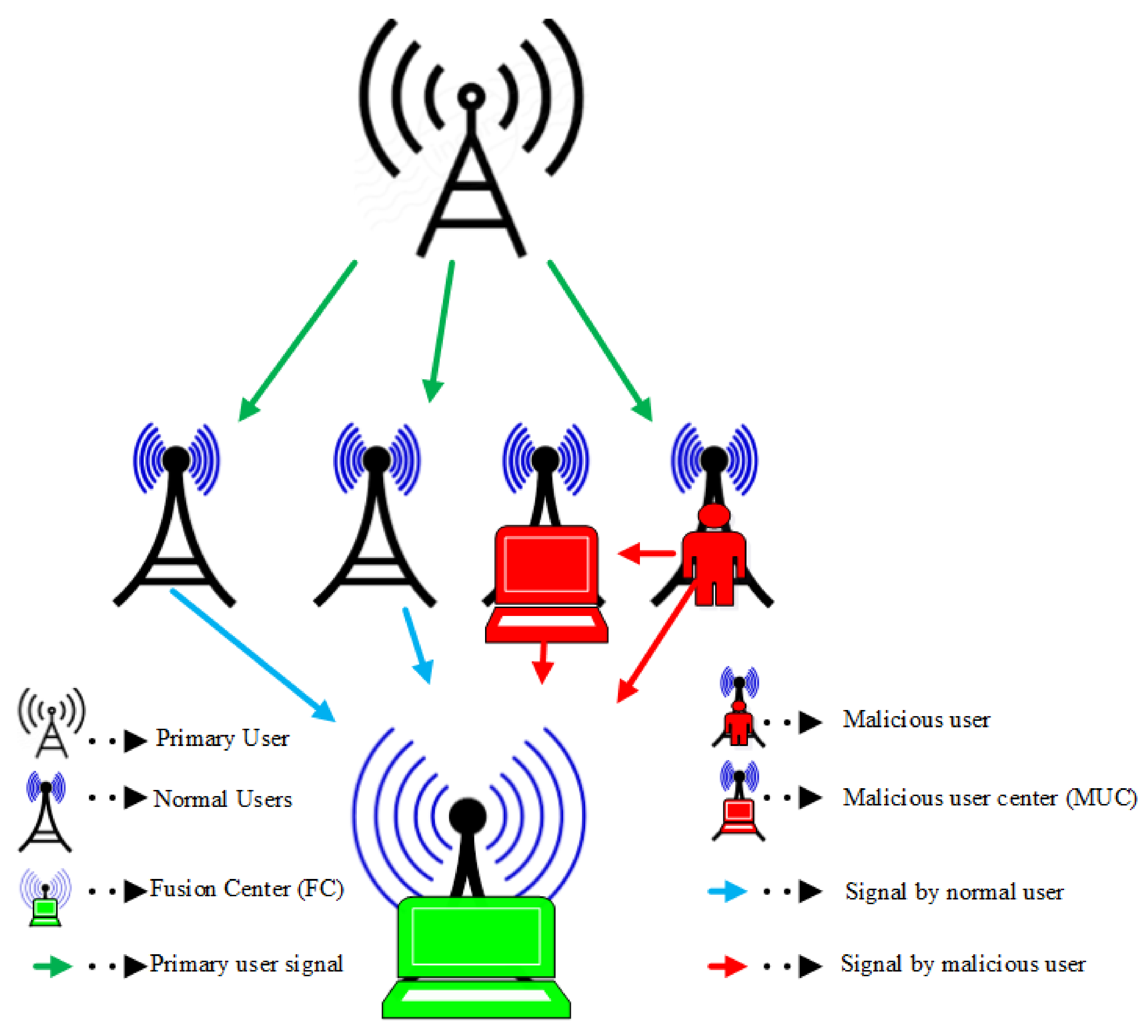
A model of the conventional centralized CSS system is shown in Figure 1. Here, the individual SUs sense the PUs’ activity and report their sensing statistics to the FC. The MUs report their observations to both the main FC and malicious user center (MUC). The MUC collusion centers in the Figure 1 combine local attacks of the individual MUs that result in more serious threats at the FC by overcoming weaknesses in the individual attackers. In this model, the MUC reports an average of the analogous MUs sensing observations to the main FC. The MUC center of the always opposite (AO) users—i.e., the always opposite collusion (AOC) center—receives sensing reports from all AO users, while the random opposite collusion (ROC) center obtains sensing data from the random opposite (RO) categories of MUs. Similarly, the MUC of an always yes (AY) user is the always yes collusion (AYC) center and the MUC anticipated for the always no (AN) users is the always no collusion (ANC) center. The participation of the AO and AOC center is implemented to reduce the network data rate and increased interference for the PU, as both the AO and AOC oppose actual PU activity in the sensing channel. As the AY reports high-energy statistics irrespective of the actual PU status, both the AY and AYC center result in increased false alarms in the system, thus decreasing network throughput. The AN user tries to sense the PU channel and inform both the main FC and ANC regarding the availability of the PU channel for access. This leads to increased interference with legitimate PU transmission. The RO and ROC centers behave similarly to the AO and AOC, which report opposite energy statistics with probability (P) and report normal sensing data with probability (1 − P). The contribution of this category of MU results in unacceptable interference and a reduced data rate for the SUs.

In the given centralized CSS, the users report their soft energy statistics to the FC to make a global decision, where soft decision fusion (SDF) is employed as a combination scheme. The challenge is to investigate the performance of the CSS in the presence of AO, AOC, AY, AYC, AN, ANC, RO, and ROC categories of MUs.

The $(H_0/H_1)$ hypothesis of the sensing channel availability presented by the $j^{th}$ SU in the $l^{th}$ sensing slot is [9]

$$\left\{\begin{array}{l}{H}_0:x_j\left(l\right)=v_j\left(l\right)\\ H_1:x_j\left(l\right)=g_{j}c\left(l\right)+v_j\left(l\right)\end{array}\right.,j\in \left\{1,2,\dots ,M\right\},l\in \left\{1,2,\dots ,K\right\},$$

(1)

where $x_j(l)$ is the $j^{th}$ user observation of the PU transmitted signal $c(l)$ with mean 0 and variance ${\sigma }_c^2$. Here, $l$ shows the sensing slot, $M$ the total number of SUs, and $K=2B{T}_s$ is the total number of samples in a bandwidth $B$ and sensing period $T_s$. $v_j(l)$ is the additive white gaussian noise (AWGN) of the channel between the PU and $j^{th}$ user that has mean zero and variance ${\sigma }_v^2$. Similarly, $g_j$ is the PU and $j^{th}$ user channel gain. The $H_0$ hypothesis in (1) states the availability of the PU channel for SU access, while the $H_1$ hypothesis is presented to show the transmission of the PU over the given sensing channel. Therefore, the SUs are allowed to gain access to the PU channel under the $H_0$ hypothesis only.

The $K$ sensing observations in (1) are combined to form the energy for the threshold detector as [9,11,45,46].

$$X_j(i)=\left\{\begin{array}{l}{\displaystyle \sum _{l=l_i}^{l_i+K-1}{\left|v_j(l)\right|}^2,\hspace{0.17em}\hspace{0.17em}\hspace{0.17em}\hspace{0.17em}\hspace{0.17em}\hspace{0.17em}\hspace{0.17em}\hspace{0.17em}\hspace{0.17em}\hspace{0.17em}\hspace{0.17em}\hspace{0.17em}\hspace{0.17em}\hspace{0.17em}\hspace{0.17em}\hspace{0.17em}{H}_0}\\ {\displaystyle \sum _{l=l_i}^{l_i+K-1}{\left|g_j\hspace{0.17em}c\hspace{0.17em}(l)+v_j(l)\right|}^2,\hspace{0.17em}\hspace{0.17em}\hspace{0.17em}{H}_1}\end{array}\right.$$

(2)

As the soft energy observation $X_j$ under both hypotheses for a sufficient number of sensing samples $K>10$ [45] closely resembles a Gaussian distribution according to the central limit theorem, (2) is rewritten as follows [9,11,45,46]:

$$X_j~\left\{\begin{array}{l}N\left({\mu }_0=K,\hspace{0.17em}{\sigma }_0^2=2K\right),\hspace{0.17em}\hspace{0.17em}\hspace{0.17em}\hspace{0.17em}\hspace{0.17em}\hspace{0.17em}\hspace{0.17em}\hspace{0.17em}\hspace{0.17em}\hspace{0.17em}\hspace{0.17em}\hspace{0.17em}\hspace{0.17em}\hspace{0.17em}\hspace{0.17em}\hspace{0.17em}\hspace{0.17em}\hspace{0.17em}\hspace{0.17em}\hspace{0.17em}\hspace{0.17em}\hspace{0.17em}\hspace{0.17em}\hspace{0.17em}{H}_0\\ N\left({\mu }_1=K(g_j+1),\hspace{0.17em}{\sigma }_1^2=2K(g_j+1)\right),\hspace{0.17em}\hspace{0.17em}\hspace{0.17em}\hspace{0.17em}{H}_1\end{array}\right.$$

(3)

where $g_j$ is the $j^{th}$ user and PU channel gain, while the mean and variance results under both the $H_0$ and $H_1$ hypotheses are $\left({\mu }_0,\hspace{0.17em}{\sigma }_0^2\right)$ and $\left({\mu }_1,{\sigma }_1^2\right)$. The energy reported from the $j^{th}$ user $Z_j$ to the FC is

$$Z_j={\displaystyle \sum _{l=1}^K{\left|U_j(l)\right|}^2}$$

(4)

where $U_j(l)=\sqrt{P_{R,j}}{h}_j{X}_j(l)+N_j(l)$ is the signal delivered to the FC using the channel between $j^{th}$ user and FC in the $l^{th}$ sensing slot. Here, $P_{R,j}$ is the $j^{th}$ SU transmission power with $h_j$ channel gain between FC and SU, whereas, the AWGN distribution has zero mean and variance ${\sigma }_j^2$, i.e., $N_j(l)~N\left(0,\hspace{0.17em}\hspace{0.17em}\hspace{0.17em}{\sigma }_j^2\right)$. Similar to the channel between the PU and SU, the SU to the FC channel noise is also assumed to be AWGN with mean zero and variance ${\delta }_j^2$.

A global decision of the PU status is generated by combining sensing reports of the $M$ SUs with the weighting coefficient vector as

$$Z(i)={\displaystyle \sum _{j=1}^M\left(w_j{Z}_j(i)\right)}$$

(5)

where $w_j$ is the weighting coefficient vector that shows the authenticity of the $j^{th}$ user sensing data, which is determined using DE. As an individual user reports statistics, $Z_j(i)$ is normally distributed, and thus the resultant $Z(i)$ is assumed to be normally distributed in nature, as in [32].

Thus,

$$E\left(Z(i)\left|H_0\right.\right)={\displaystyle \sum _{j=1}^M{w}_{j}K{\sigma }_{0,j}^2}$$

(6)

$$E\left(Z(i)\left|H_1\right.\right)={\displaystyle \sum _{j=1}^M{w}_{j}K{\sigma }_{1,j}^2}$$

(7)

$$Var\left(Z(i)\left|H_0\right.\right)={\displaystyle {\sum }_{j=1}^{M}2w_j^{2}K{({\sigma }_{0,j}^2+{\delta }_j^2)}^2}={\overrightarrow{w}}^T\hspace{0.17em}{\mathsf{\Phi }}_{H_0}\overrightarrow{w}$$

(8)

$$Var\left(Z(i)\left|H_1\right.\right)={\displaystyle {\sum }_{j=1}^{M}2w_j^{2}K{({\sigma }_{1,j}^2+{\sigma }_{0,j}^2)}^2}={\overrightarrow{w}}^T\hspace{0.17em}{\mathsf{\Phi }}_{H_1}\overrightarrow{w}$$

(9)

In (6) and (7), ${\sigma }_{0,j}^2$ and ${\sigma }_{1,j}^2$ are $U_j(l)$ variances under $H_0/H_1$ of the $j^{th}$ user, where ${\sigma }_{0,j}^2=P_{R,j}\left|h_j\right|{\sigma }_{v_j}^2+{\delta }_j^2$ and ${\sigma }_{1,j}^2=P_{R,j}{\left|g_j\right|}^2{\left|h_j\right|}^2{\sigma }_c^2+{\sigma }_{0,j}^2$.

The goal is then to find an optimal coefficient vector that can help in determining the appropriate threshold $\beta$ with minimum sensing error. These optimal weighting coefficients help us to train the BTA scheme in the description of the proposed model.

The $H_0/H_1$ hypotheses result in the following covariance matrices:

$${\mathsf{\Phi }}_{H_0}=diag\left(2K{\sigma }_{0,j}^4\right)$$

(10)

$${\mathsf{\Phi }}_{H_1}=diag\left(2K{(P_{R,j}|g_j{|}^2|h_j{|}^2{\sigma }_S^2+{\sigma }_{0,j}^2)}^2\right)$$

(11)

where ${\sigma }_{0,j}^2$ and ${\sigma }_{1,j}^2$ represent square diagonal matrices in (10) and (11).

The detection and false alarm probabilities show the occupancy of the licensee channel by the PU and the idle status when it is falsely identified to be in use by the licensee as

$$P_f=P\left(Z(i)>\beta \left|H_0\right.\right)=Q\left(\frac{\beta -E(Z(i)\left|H_0)\right.}{\sqrt{\mathrm{var}(Z(i)\left|H_0)\right.}}\right)=Q\left(\frac{\beta -{\overrightarrow{w}}^T{\overrightarrow{\mu }}_0}{\sqrt{{\overrightarrow{w}}^T{\mathsf{\Phi }}_{H_0}\overrightarrow{w}}}\right)$$

(12)

$$P_d=P\left(Z(i)>\beta \left|H_1\right.\right)=Q\left(\frac{\beta -E(Z(i)\left|H_1)\right.}{\sqrt{\mathrm{var}(Z(i)\left|H_1)\right.}}\right)=Q\left(\frac{\beta -{\overrightarrow{w}}^T{\overrightarrow{\mu }}_1}{\sqrt{{\overrightarrow{w}}^T{\mathsf{\Phi }}_{H_1}\overrightarrow{w}}}\right)$$

(13)

where $\beta$ is the optimal threshold, represented as

$$\beta =\left(\frac{\sqrt{w^T{\mathsf{\Phi }}_{H_1}w}{\mu }_0^T\overrightarrow{w}+\sqrt{\overrightarrow{w}{\mathsf{\Phi }}_{H_1}w}{\mu }_1^{T}w}{\sqrt{w^T{\mathsf{\Phi }}_{H_0}w}+\sqrt{w^T{\mathsf{\Phi }}_{H_1}w}}\right)$$

(14)

Assuming the false alarm probability to be $P_f=1-P_d$ and $P_f=P_m$, where $P_m$ is the misdetection probability, the total error probability $P_e$ is determined as follows:

$$P_e=P_f+P_m=Q\left(\frac{\beta -{\overrightarrow{w}}^T{\overrightarrow{\mu }}_0}{\sqrt{{\overrightarrow{w}}^T{\mathsf{\Phi }}_{H_0}\overrightarrow{w}}}\right)+Q\left(\frac{{\overrightarrow{w}}^T{\overrightarrow{\mu }}_1-\beta }{\sqrt{{\overrightarrow{w}}^T{\mathsf{\Phi }}_{H_1}\overrightarrow{w}}}\right)$$

(15)

The error probability in (15) depends on the selection of $\overrightarrow{w}$. The optimal threshold $\beta$ using (14) is substituted in (12), (13), and (15), which produces the minimum false alarm, high detection, and low error probability results.

Using the proposed scheme, we see in the following section that $0<w_j(i)<1$ and $\sqrt{{\displaystyle \sum _{j=1}^M{w}_j^2(i)}}=1$, in order to reduce the selection procedure of the search space for the DE.

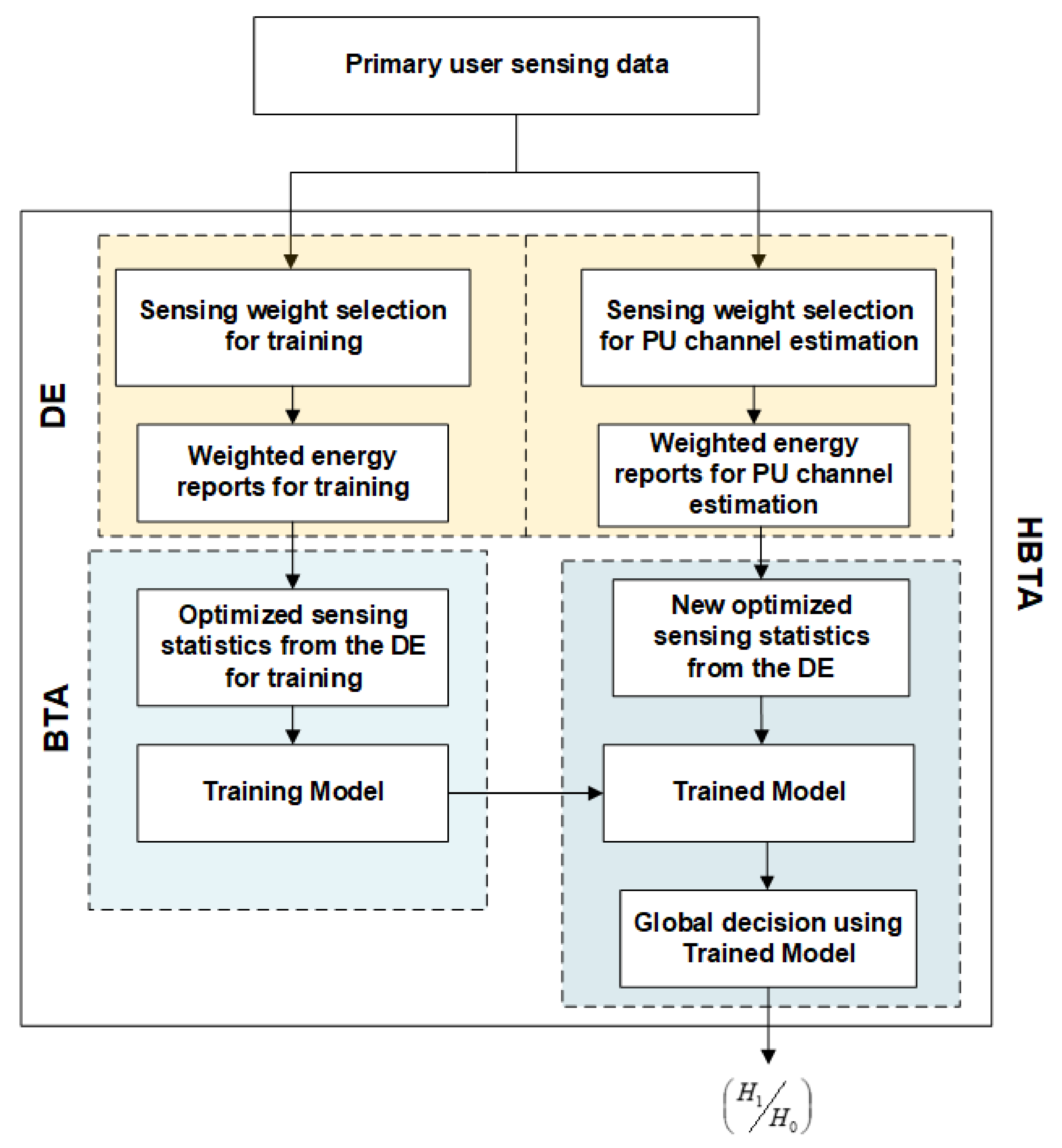
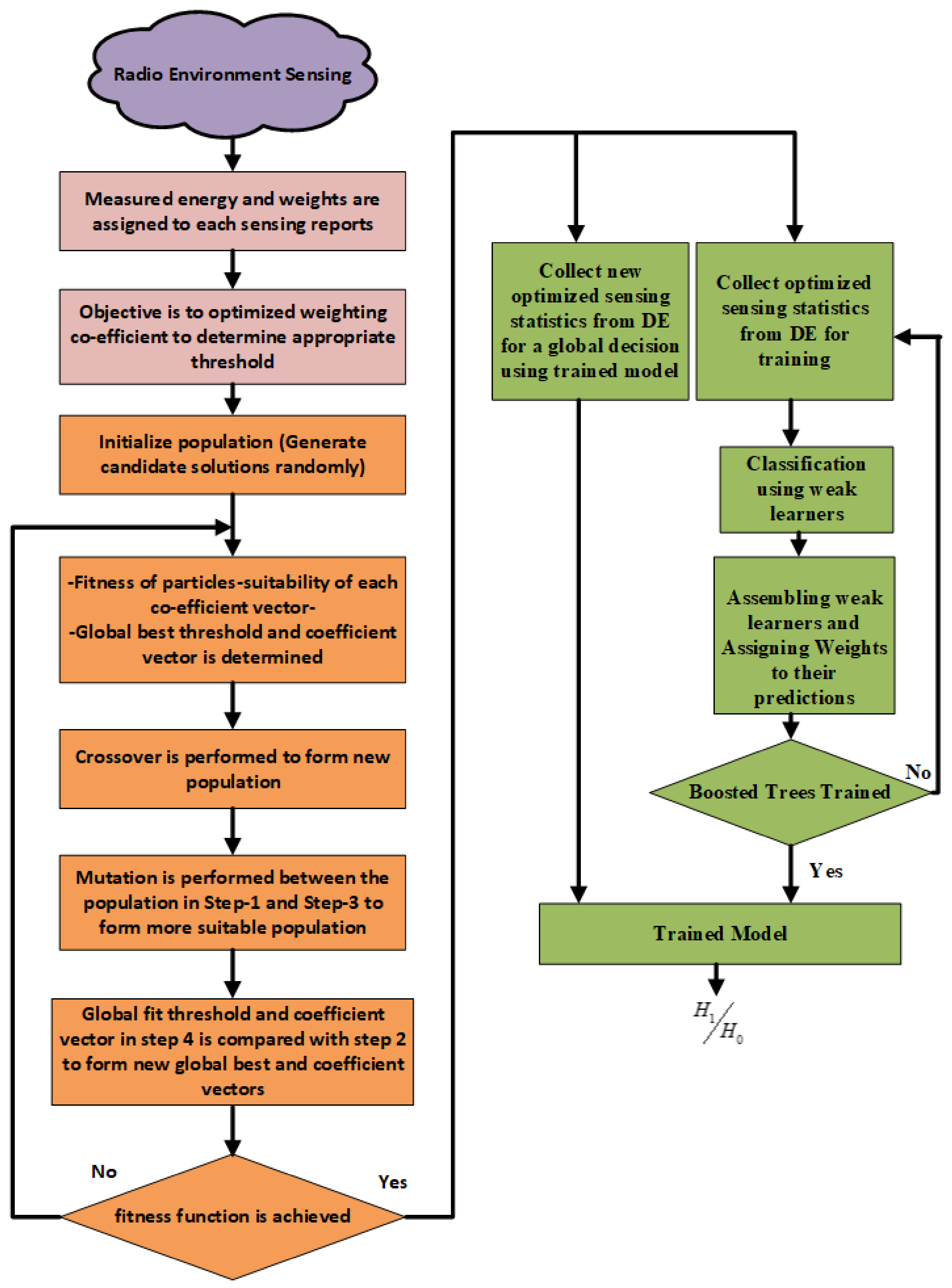
3. Proposed Hybrid Boosted Tree Algorithm

In the proposed model, we use the DE scheme to select weighting coefficients against the SUs by assigning high weights to normal users and minimum significance to the sensing of MUs. The optimal weighting coefficients identified in the first part are further utilized to train the BTA scheme.

Unlike the training procedure in [44], where the reporting users’ soft energy information is used to train the BTA, this work collects both soft energy reports of the users along with optimal coefficient vectors from the DE, allowing the BTA to rely strongly on the sensing decisions of the normal SUs. An abstract block diagram of the proposed method is shown in Figure 2.

3.1. Differential Evolution-Based Solution

DE is a population-based search algorithm following crossover, mutation, and selection methods as in [8,43]. The major difference between DE and other optimization algorithms, while searching for the best fitness, is that DE selection depends on mutation. In addition, DE uses a non-uniform crossover, where child vector parameters of one parent are taken into consideration strongly in comparison with other parents. The DE has the ability to identify the global minimum irrespective of some initial parameters and exhibits quick convergence to the problem solution with fewer control parameters.

The self-adaptability in DE introduced via the mutation and selection procedure is its major advantage. Storm and Price were the first to suggest DE as a population-based stochastic search algorithm for the optimization of continuous functions in [47].

In this part of the proposed scheme, DE is employed to determine the optimal coefficient vector against the users’ reporting statistics. The selected coefficient vector in the final stage of the DE assigns a high weight to the sensing of a normal user to make their reports more authentic. Similarly, different categories of MUs are charged with minimum weights that enable the FC to rely on the reports of normal sensing users. The steps involved in DE finding an optimal threshold and coefficient vectors are as follows.

Step 1: Initialization

In this work, a total of $N$ candidate solutions (individuals) for DE have been considered. The algorithm starts with a population initialization that has $N$ candidate solutions and $M$ dimensions equal to the total number of SUs; i.e., ${\overrightarrow{w}}_x={\left[w_1 w_2\dots w_M\right]}^T, x\in 1,\dots ,N$:

$$w_x=L+\left(H-L\right)\times rand\left(N,\hspace{0.17em}M\right)$$

(16)

where $L$ and $H$ are the lower and upper limits of the $x$ coefficient vector. The fitness value of each coefficient vector is determined in terms of the error probabilities $P_e({\overrightarrow{w}}_x(1)\hspace{0.17em}),\hspace{0.17em}{P}_e({\overrightarrow{w}}_x(2)\hspace{0.17em}),\dots ,\hspace{0.17em}{P}_e({\overrightarrow{w}}_x(N)\hspace{0.17em})$. Therefore, the vector with the minimum error probability out of all $N$ vectors is selected along with corresponding threshold β value as an optimal threshold.

Step 2: Random Numbers Selection

In the second step, dissimilar random numbers n₁, n₂, n₃ are produced such that none of them is equal to any other.

Step 3: Mutation

In this step, the initial population, $w_x$, and dissimilar random numbers $n_1,n_2,n_3$ from step 2 are used to generate a new population as

$$w_y=w_x(n_1)+F\times (w_x(n_2)-w_x(n_3))$$

(17)

where $w_y$ is the mutant or mutation vector. The difference employed in the result of (17) forms the given algorithm DE. The selection of the constant number, $F$, is dependent on the problem, which is placed to keep the value of genes in the range of $L$ and $H$.

Step 4: Crossover

A crossover operation is performed in this step using $w_x$ and the mutant vector, $w_y$, to select genes among $w_x$ and $w_y$ as

$$w_z=\left\{\begin{array}{l}{w}_y\hspace{0.17em}\hspace{0.17em}\hspace{0.17em}if\hspace{0.17em}\hspace{0.17em}{a}_j\le CR\hspace{0.17em}\hspace{0.17em}or\hspace{0.17em}j=jrand\\ w_x\hspace{0.17em}\hspace{0.17em}\hspace{0.17em}\hspace{0.17em}otherwise\end{array}\right\}$$

(18)

where $a_j$ is a uniformly distributed random number between 0 and 1, while $j$ is the element number of the candidate solution and $jrand$ is an integer randomly selected from 1 to $M$. Similarly, the value of $CR$ in (18) is $0\le CR\le 1$.

Step 5: Particles Fitness

The suitability of the $w_z$ coefficient vectors is determined in this step using the error probabilities $P_e\hspace{0.17em}(\hspace{0.17em}{\overrightarrow{w}}_z\hspace{0.17em}(\hspace{0.17em}1\hspace{0.17em})\hspace{0.17em}\hspace{0.17em}),\hspace{0.17em}{P}_e\hspace{0.17em}({\overrightarrow{w}}_z\hspace{0.17em}(\hspace{0.17em}2\hspace{0.17em})\hspace{0.17em}),\dots ,\hspace{0.17em}\hspace{0.17em}{P}_e(\hspace{0.17em}{\overrightarrow{w}}_z\hspace{0.17em}(N)\hspace{0.17em})$. Therefore, the coefficient vector with the minimum error probability is identified as the new global best vector and its associated threshold, $\beta$, is selected as the new global best threshold.

Step 6: Population and Global Best Vector Up-Gradation

The fitness values of $w_z$ is compared with the initial population, $w_x$, to search for any up-gradation as

$$w_x=\left\{\begin{array}{l}{w}_z\hspace{0.17em}\hspace{0.17em}\hspace{0.17em}\hspace{0.17em}\hspace{0.17em}Fitness\hspace{0.17em}(w_z)>Fitness\hspace{0.17em}(w_x)\\ w_x\hspace{0.17em}\hspace{0.17em}\hspace{0.17em}\hspace{0.17em}otherwise\end{array}\right\}$$

(19)

Similarly, the fitness of the new global best in $w_z$ is compared with that of $w_x$ to upgrade the global best and optimum threshold results accordingly.

Step 7: Stopping Criteria

In this step, a check is made to start recycling DE in step 2 or to end the DE process by inspecting the fitness function; i.e., whether the minimum error probability results have been achieved or the required number of iterations has been reached. The algorithm finally returns the global best coefficient vector and optimum threshold results.

3.2. Boosted Tree Algorithm

The working principle used by the BTA to solve the given problem is categorized into three major steps.

In the first step, $N$ sensing observations consisting of user energy statistics along with coefficient vectors from the DE are collected at the FC and stored as feature vectors for the proposed BTA scheme. In step 2, the BTA is trained with the AdaBoost ensembling method. A more suitable and accurate decision is made using the BTA by accumulating and strengthening weak classifiers in this step. The detection and false alarm probabilities in step 3 are determined by considering the results in step 2 to make a global decision.

Step 1: Data Matrix Formulation

A history-reporting matrix is formed at the FC, consisting of a combination of individual users’ soft energy statistics and weighting coefficient vectors, as shown below.

$$S=\left[s_{ij}\right]=\left[\begin{array}{llll}{s}_{11}\hfill & s_{12}\hfill & \dots \hfill & s_{1M}\hfill \\ s_{21}\hfill & s_{22}\hfill & \dots \hfill & s_{2M}\hfill \\ s_{31}\hfill & s_{32}\hfill & \dots \hfill & s_{3M}\hfill \\ \hspace{0.17em}\hspace{0.17em}⋮\hfill & \hspace{0.17em}\hspace{0.17em}⋮\hfill & \ddots \hfill & \hspace{0.17em}\hspace{0.17em}⋮\hfill \\ s_{N1}\hfill & s_{N2}\hfill & \cdots \hfill & s_{NM}\hfill \end{array}\right],i\in \left\{1,2,\dots ,N\right\},j\in \left\{1,2,\dots ,M\right\},$$

(20)

where $s_{ij}=Z_j(i)\times w_j(i)$ is the $j^{th}$ user’s sensing statistics in combination with the $j^{th}$ component of the coefficient vector. The $M$ users sensing data including both normal and malicious participants are accumulated in $N$ sensing periods with $K$ sensing samples. The spectrum sensing falsification effects of MUs are minimized by the proposed technique in the following steps. The ML algorithms can find natural patterns in the data, which helps in decision making and produces improved prediction results.

Step 2: BTA Training Phase

The BTA scheme proposed in this paper uses adaptive boosting (AdaBoost) as an ensemble method, where weak classifiers are ensembled to make a strong classifier. The training set consists of $T={\left\{\left(s_{ij},y_i\right)\right\}}_{i=1}^N,\hspace{0.17em}{s}_{ij}\in {\Re }^N,\hspace{0.17em}\hspace{0.17em}{y}_i\in \left\{-1,\hspace{0.17em}1\right\}$, where $y_i=1$ represents the class label presence of PU activity, whereas $y_i=-1$ denotes the availability of the PU channel for SU access. The training set $T$ is constructed as an $N\times \left(M+1\right)$ with dimensional space $T\in {\Re }^{N\times (M+1)}$ and is written as

$$T=\left[\left.\begin{array}{cccc}{s}_{11}& s_{12}& \dots & s_{1M}\\ s_{21}& s_{22}& \dots & s_{2M}\\ ⋮& ⋮& \ddots & ⋮\\ s_{N1}& s_{N2}& \dots & s_{NM}\end{array}\right|\begin{array}{c}{y}_1\\ y_2\\ ⋮\\ y_N\end{array}\right],$$

(21)

where $s^1={\left[\begin{array}{c}{s}_{11}\\ s_{12}\\ ⋮\\ s_{1M}\end{array}\right]}^T$, $s^2={\left[\begin{array}{c}{s}_{21}\\ s_{22}\\ ⋮\\ s_{2M}\end{array}\right]}^T$, $s^3={\left[\begin{array}{c}{s}_{31}\\ s_{32}\\ ⋮\\ s_{3M}\end{array}\right]}^T$ and $s^N={\left[\begin{array}{c}{s}_{N1}\\ s_{N2}\\ ⋮\\ s_{NM}\end{array}\right]}^T$ are the $N$ feature vectors used to train the BTA scheme consisting of weighted soft energy reports of the $M$ SUs. The training set, $T$, consists of two sub matrices, $S$ and $Y$, where sub matrix $S\in {\Re }^{N\times M}$ is the matrix of the weighted soft energy statistics of the users’ data, while $Y\in {\Re }^{N\times 1}$ are the $N$ label (targets) values of the actual PU activity.

In this work, a total of $k$ classifiers at the FC participate in making sensing decisions in case $s^i$ is used as the $i^{th}$ feature vector. The different classifiers used here try to predict a class label for the feature vector $s^i$, where the final output is determined using a linear combination of the label estimation predicted by different classifiers. In the linear combination, each individual term is the product of the classifiers’ predicted value and the weight assigned to the classifier-predicted values. AdaBoost is a boosted classifier such that each $k^{th}$ classifier is assigned decision weights, while taking into consideration the already known predicted (k − 1) classifiers as

$$e_{k-1}\left(s^i\right)={\displaystyle \sum _{p=1}^{k-1}{\alpha }_p{h}_p\left(s^i\right)},\hspace{0.17em}p\in \left\{1,2,\dots ,k-1\right\},\hspace{0.17em}\hspace{0.17em}i\in \left\{1,\dots ,N\right\},$$

(22)

where $h_p(s^i)$ is the prediction of the $p^{th}$ classifier and ${\alpha }_p$ is the weight assigned to the predicted value of the $p^{th}$ classifier.

The prediction performance of the $k^{th}$ classifier is combined with $h_k(s^i)$ as the predicted value of the classifier and ${\alpha }_k$ as the optimum weight of the classifier to establish a better boosted classifier. To determine ${\alpha }_k$, the process is as follows:

$$e_k(s^i)={\displaystyle \sum _{p=1}^{k-1}{\alpha }_p{h}_p(s^i)}+{\alpha }_k{h}_k(s^i)$$

(23)

Similarly, (23) is written using the value from (22) as

$$e_k(s^i)=e_{k-1}(s^i)+{\alpha }_k{h}_k(s^i)$$

(24)

where $e_k\left(s^i\right)$ is the compound predicted value aggregated through the prediction results of the $k$ classifiers. The aim is to form a closed form formula for ${\alpha }_k$ that assigns ${\alpha }_k$ a value such that the total prediction error is minimized. As the total prediction error in AdaBoost is equal to the sum of the negative natural exponent of $y^i{e}_k(s^i)$ for all training examples [48] as

$$E={\displaystyle \sum _{i=1}^n{e}^{-y^i\left[e_{k-1}(s^i)+{\alpha }_k{h}_k\left(s^i\right)\right]}},$$

(25)

the representation of the total prediction error, $E$, now takes the form below:

$$E={\displaystyle \sum _{i=1}^n{w}_k^i{e}^{-y^i{\alpha }_k{h}_k\left(s^i\right)}}$$

(26)

where $w_k^i=e^{-y^i{e}_{k-1}(s^i)}$ is the corresponding weight in the case of a classifier number of $k>1$. The total prediction error, $E$, in (26) is split into cases with correct prediction as $(y^i{h}_k(s^i)=1)$ and the case that leads to an incorrect prediction $(y^i{h}_k(s^i)=-1)$ as

$$\begin{gathered} E\hspace{0.17em}\hspace{0.17em}\hspace{0.17em}\hspace{0.17em}={\displaystyle \sum _{y^i=h(s^i)}{w}_c{e}^{-y^i{\alpha }_k{h}_k(s^i)}+}{\displaystyle \sum _{y^i\ne h(s^i)}{w}_e{e}^{-y^i{\alpha }_k{h}_k(s^i)}}, \\ ={\displaystyle \sum _{y^i=h(s^i)}{w}_c{e}^{-{\alpha }_k}}+{\displaystyle \sum _{y^i\ne h(s^i)}{w}_e{e}^{{\alpha }_k}}, \\ =\hspace{0.17em}\hspace{0.17em}\hspace{0.17em}{e}^{-{\alpha }_k}{\displaystyle \sum _{y^i=h_k(s^i)}{w}_c\hspace{0.17em}+\hspace{0.17em}}\hspace{0.17em}{e}^{{\alpha }_k}{\displaystyle \sum _{y^i\ne h_k(s^i)}{w}_e}, \\ =\hspace{0.17em}\hspace{0.17em}\hspace{0.17em}\hspace{0.17em}{W}_c\hspace{0.17em}{e}^{-{\alpha }_k}+W_e\hspace{0.17em}{e}^{{\alpha }_k}, \end{gathered}$$

(27)

where $W_c\hspace{0.17em}\hspace{0.17em}=\hspace{0.17em}{\displaystyle \sum _{y^i=\hspace{0.17em}{h}_k(s^i)}{w}_c}$ and $W_e\hspace{0.17em}\hspace{0.17em}=\hspace{0.17em}{\displaystyle \sum _{y^i\ne \hspace{0.17em}{h}_k(s^i)}{w}_e}$. The object is to minimize the loss function, $E$, for the chosen weak classifier, $h_k$, selected earlier. Thus, the total error of prediction, $E$, is differentiated with the classifier weight, ${\alpha }_k$, where the minimization condition is set to zero as

$$\frac{\partial E({\alpha }_k)}{\partial {\alpha }_k}=0$$

(28)

As in (27), the minimization of the total error with reference to ${\alpha }_k$ is the same as if we minimize $\left(W_c{e}^{-{\alpha }_k}+W_e{e}^{{\alpha }_k}\right)$ with respect to ${\alpha }_k$:

$$\frac{\partial E({\alpha }_k)}{\partial {\alpha }_k}=-W_c{e}^{-{\alpha }_k}+W_e{e}^{{\alpha }_k}$$

(29)

The solution of (29) in terms of ${\alpha }_k$ is as follows:

$${\alpha }_k=\frac{1}{2}\ln \left(\frac{W_c}{W_e}\right)$$

(30)

As $W_c=W-W_e$, with $W$ the total sum of the weights, therefore, is

$${\alpha }_k=\frac{1}{2}\ln \left(\frac{W-W_e}{W_e}\right)$$

(31)

Finally, the expression for weight ${\alpha }_k$ in its final form is

$${\alpha }_k=\frac{1}{2}\ln \left(\frac{1-e_m}{e_m}\right)$$

(32)

where $e_m=\raisebox{1ex}{$W_e$}\!\left/ \!\raisebox{-1ex}{$W$}\right.$ is the weighted error rate of the weak classifier $h_k$.

Step 3: Global Decision Using Proposed Scheme

There are a several combination schemes that should be employed at the FC while making a global decision. These include equal gain combination (EGC) and maximum gain combination (MGC). The EGC scheme assigns equal weights to the sensing reports of all SUs as

$$G_{EGC}(i)=\left\{\begin{array}{l}{H}_1:\hspace{0.17em}\hspace{0.17em}\hspace{0.17em}\hspace{0.17em}\hspace{0.17em}\hspace{0.17em}\hspace{0.17em}\hspace{0.17em}\frac{1}{M}{\displaystyle \sum _{j=1}^M{s}_j(i)}\ge \gamma \\ H_0:\hspace{0.17em}\hspace{0.17em}\hspace{0.17em}\hspace{0.17em}\hspace{0.17em}\hspace{0.17em}\hspace{0.17em}\hspace{0.17em}\hspace{0.17em}\hspace{0.17em}otherwise\end{array}\right.$$

(33)

The MGC scheme at the FC observes sensing reports from different branches and assign a high weight to users with high SNR reports, while the low SNR reports receive minimum weights. Thus, strong signal branches receive amplification and branches with weak signals are further weakened as

$$G_{MGC}(i)=\left\{\begin{array}{l}{H}_1:{\displaystyle \sum _{j=1}^M\left(e_j\times s_j(i)\right)\ge \gamma }\\ H_0:\hspace{0.17em}\hspace{0.17em}otherwise\end{array}\right.$$

(34)

where $e_j=\frac{g(j)}{{\displaystyle \sum _{j=1}^{M}g(j)}}$.

The system is trained based on users’ reported sensing data received from all SUs and the optimum coefficient vector identified using DE. The HBTA considers the following sensing observations and coefficient vectors of the DE to make the final PU channel predictions as

$$G_{BTA}(i)=\left\{\begin{array}{l}{H}_1:\hspace{0.17em}\hspace{0.17em}\hspace{0.17em}\hspace{0.17em}\mathrm{HBTA}\hspace{0.17em}\hspace{0.17em}(s^i)=1\\ H_0:\hspace{0.17em}\hspace{0.17em}\hspace{0.17em}\hspace{0.17em}otherwise\end{array}\right.\hspace{0.17em}\hspace{0.17em},$$

(35)

where HBTA refers to the trained hybrid BTA algorithm that takes a new input feature vector, $s^i$, to estimate the occupancy of the PU channel. $G_{BTA}$ is a global decision of the hybridized HBTA scheme. The channel is considered occupied if $\mathrm{HBTA}\hspace{0.17em}(s^i)=1$ results in 1; otherwise, the channel is considered vacant. Detection and false alarm probabilities at the FC based on (35) are calculated as

$$\begin{array}{l}{P}_{d-HBTA}=\mathrm{Pr}\left\{G_{HBTA}(i)=1\left|H_1\right.\right\}=\mathrm{Pr}\left\{\mathrm{HBTA}\hspace{0.17em}(s^i)=1\left|H_1\right.\right\},\\ P_{f-HBTA}=\mathrm{Pr}\left\{G_{HBTA}(i)=1\left|H_0\right.\right\}=\mathrm{Pr}\left\{\mathrm{HBTA}\hspace{0.17em}(s^i)=1\left|H_0\right.\right\}.\end{array}$$

(36)

An flowchart diagram of the proposed HBTA scheme is shown in Figure 3.

4. Simulation Results

In the simulations, the total number of SUs was kept at 14 to observe the changes in error probability concerning SNRs, sensing samples, the population size of the algorithm, and the number of iterations. The SNRs varied in the range of −20 dB to +20 dB, while the iterations of the algorithm changed from 50 to 110. Similarly, the population size varied in the range of 20 to 80, while the sensing samples changed from 270 to 335. The SUs were placed in different SNRs to sense the PU channel independently. The genetic algorithm (GA) and particle swarm optimization (PSO) showed the total number of N chromosomes with M total gene bits. The maximum number of sensing iterations of the GA and PSO was kept at 50. Similarly, the GA crossover rate was randomly selected in the range of 1 to $M$. The performance of the proposed HBTA-based SDF algorithm was compared with the PSO, GA, DE, BTA and KNN-based SDF combination schemes.

The simulation environment was divided into six different cases. Case 1 showed the probability of error results against varying algorithm iterations. Case 2 showed the probability of error results with the contribution of varying population sizes. Similarly, Case 3 showed the error probability results with increasing sensing samples. Case 4 explored the total probability of error results versus varying SNRs at two different iteration levels. The results of the error probability at varying SNRs and with two different population sizes were explored in Case 5. Finally, Case 6 showed the error probabilities with two different sensing samples and a fixed population size, iteration number, and total number of users.

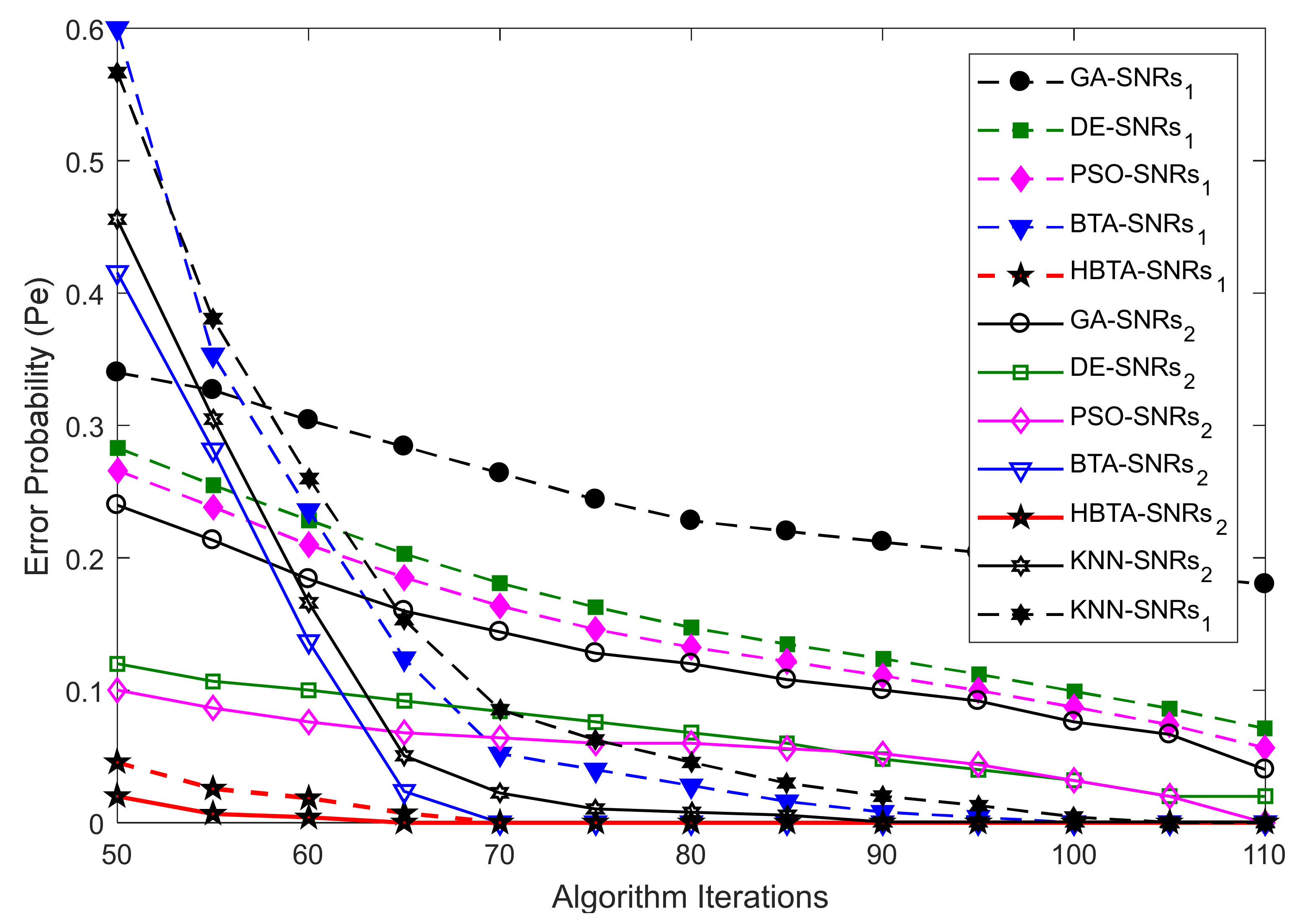
Case 1:

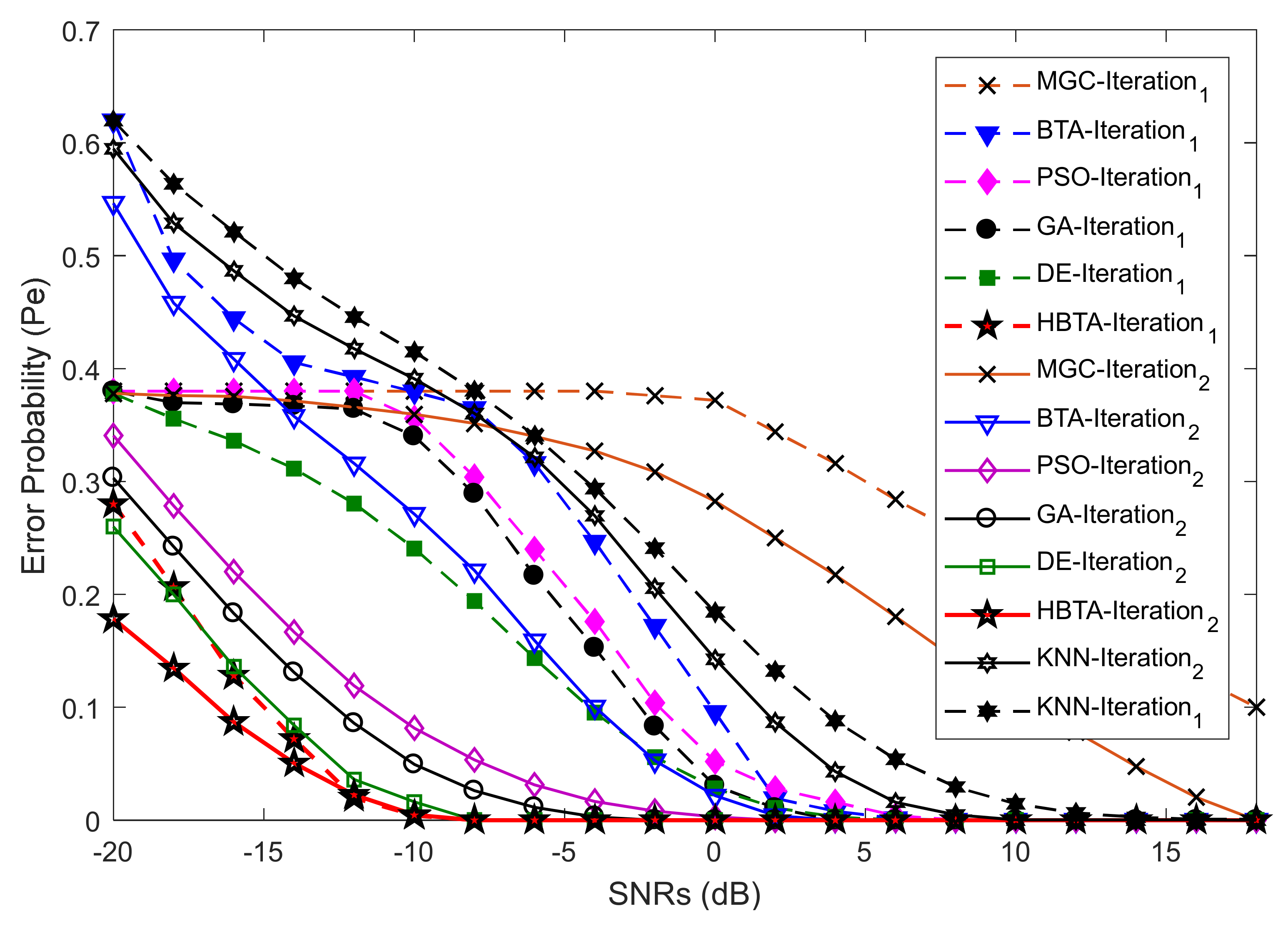
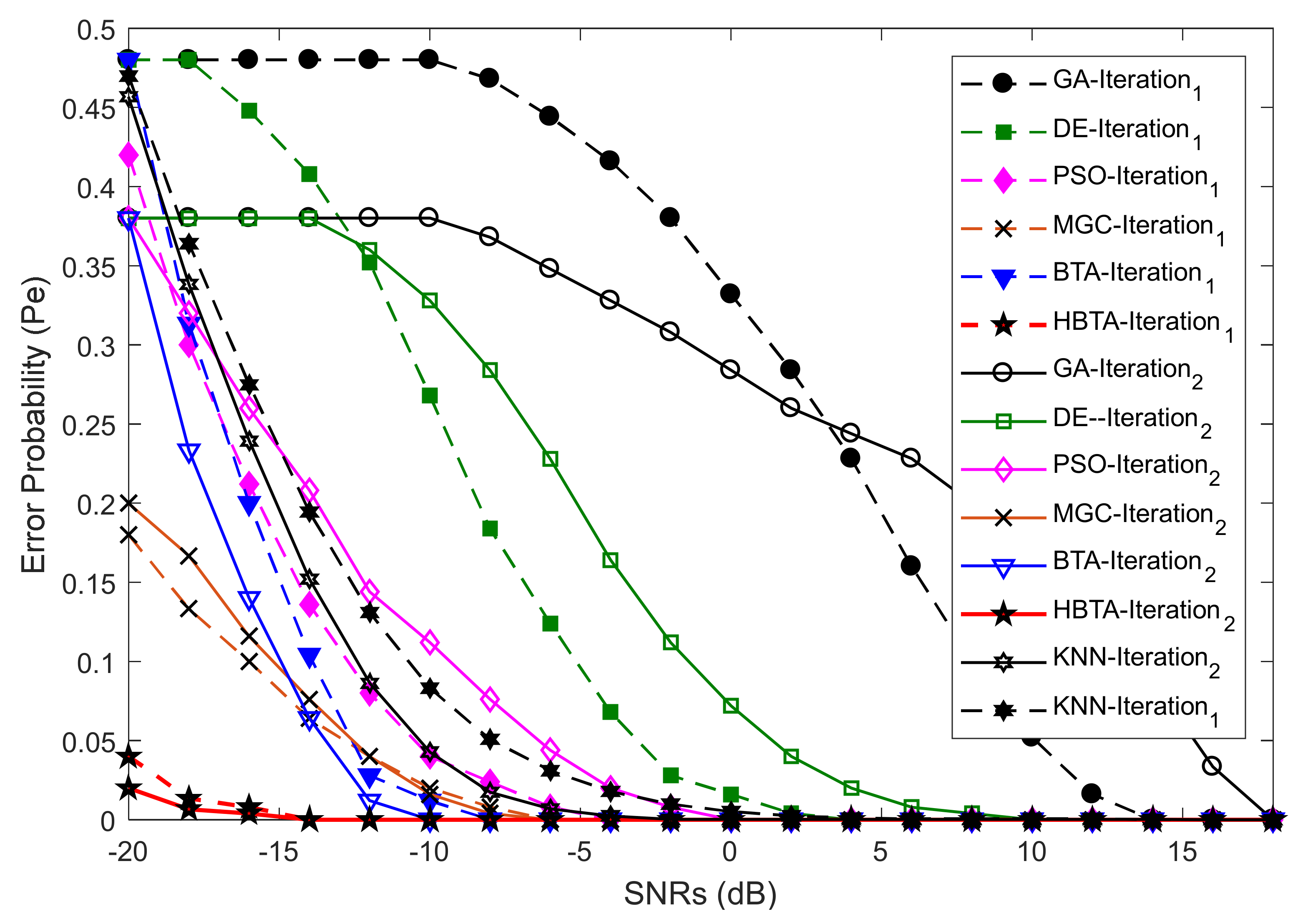
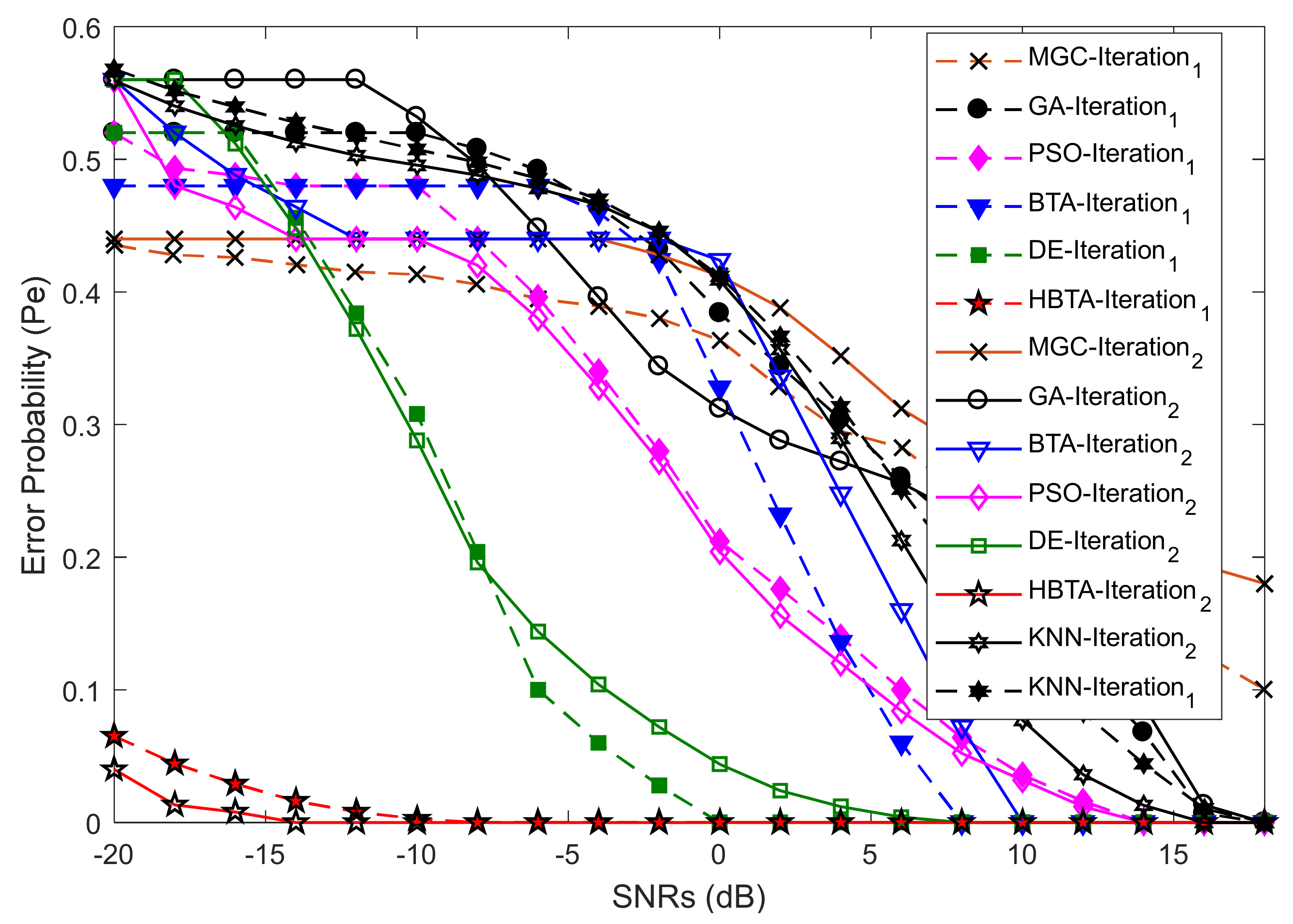
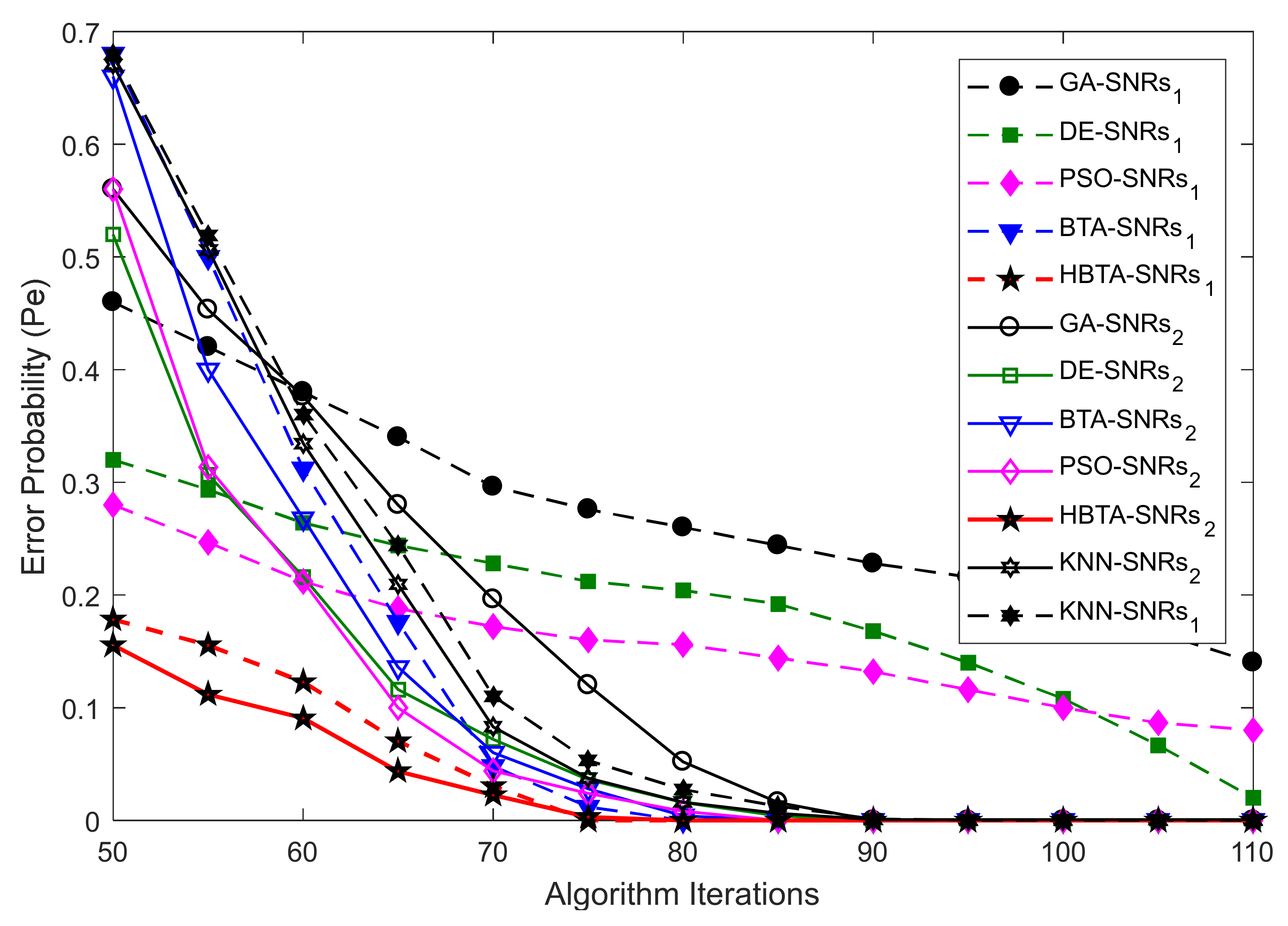
In this part of the simulation, the error probability was determined against an increasing number of algorithm iterations. The SNRs, algorithm population, sensing samples, and the total number of SUs were kept constant, as shown in Figure 4, Figure 5 and Figure 6. In Figure 4, the error probability results are compared for the GA, DE, PSO, BTA, KNN, and HBTA schemes against varying iteration levels at average SNRs of −9.5 dB and −0.5 dB. The result in Figure 4 shows that the proposed HBTA scheme exhibited better sensing performance with minimum sensing error compared with the other schemes at different iteration levels in the presence of the AY category of MUs. 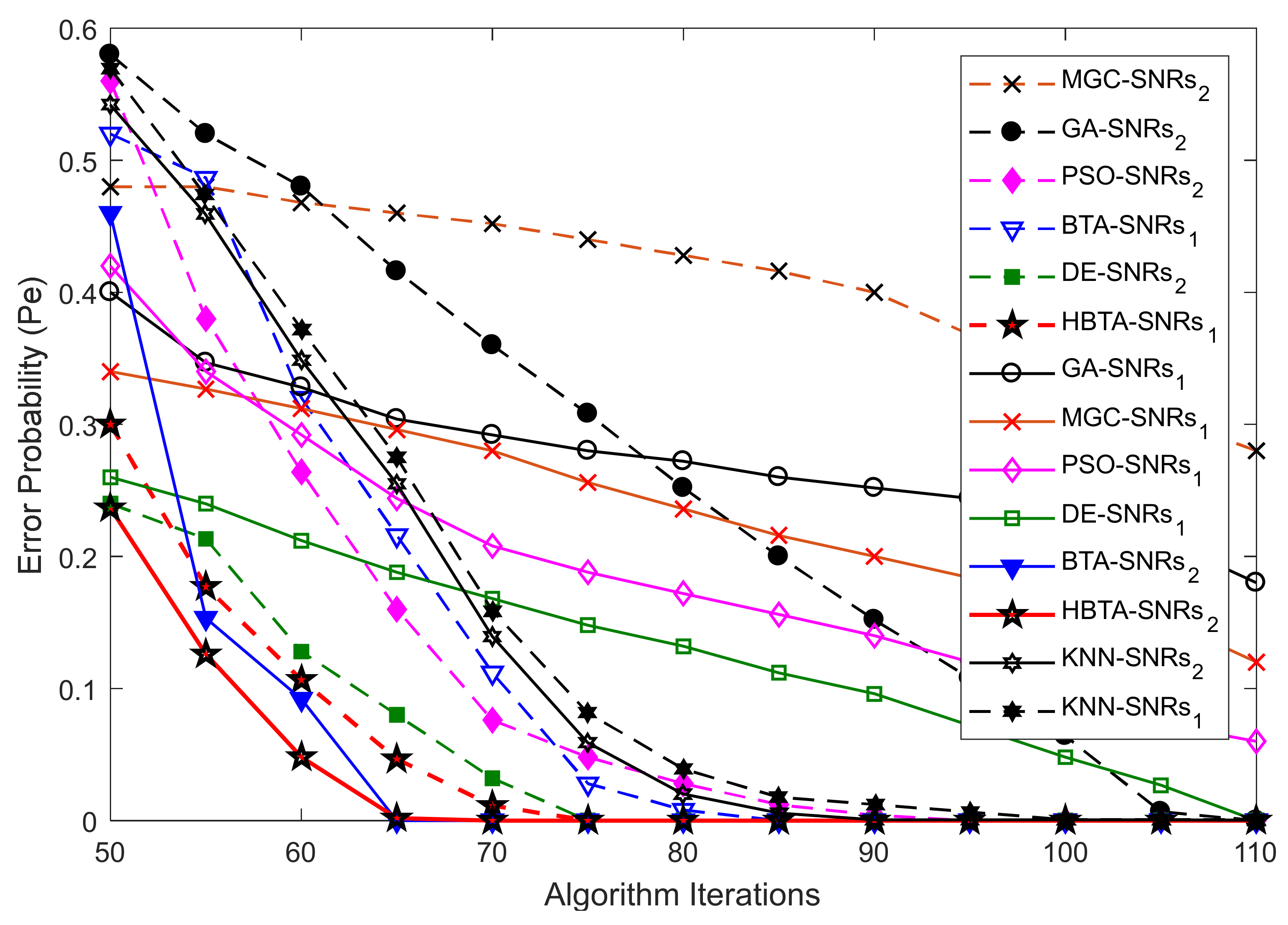The results in Figure 5 were collected in the presence of an AN-ANC user in CSS. These results show improved sensing performance with the proposed HBTA scheme, followed by the PSO, DE, KNN, and simple BTA schemes. The simple GA scheme showed the worst sensing performance, with high sensing error in the presence of the AN-ANC category of MUs. Similarly, the effects of an AO-AOC user in terms of misleading the FC’s decision about the PU channel is investigated in Figure 6. The results in Figure 6 show the error probability against varying algorithm iterations at two different average SNRs of −0.5 dB and −9.5 dB with a fixed population size and total number of users. It is clear from the graphical illustrations in Figure 6 that the proposed HBTA scheme showed better performance for all algorithm iterations followed by the simple BTA scheme and KNN in terms of sensing. The GA and MGC-SDF schemes showed poor sensing performance with high sensing error.

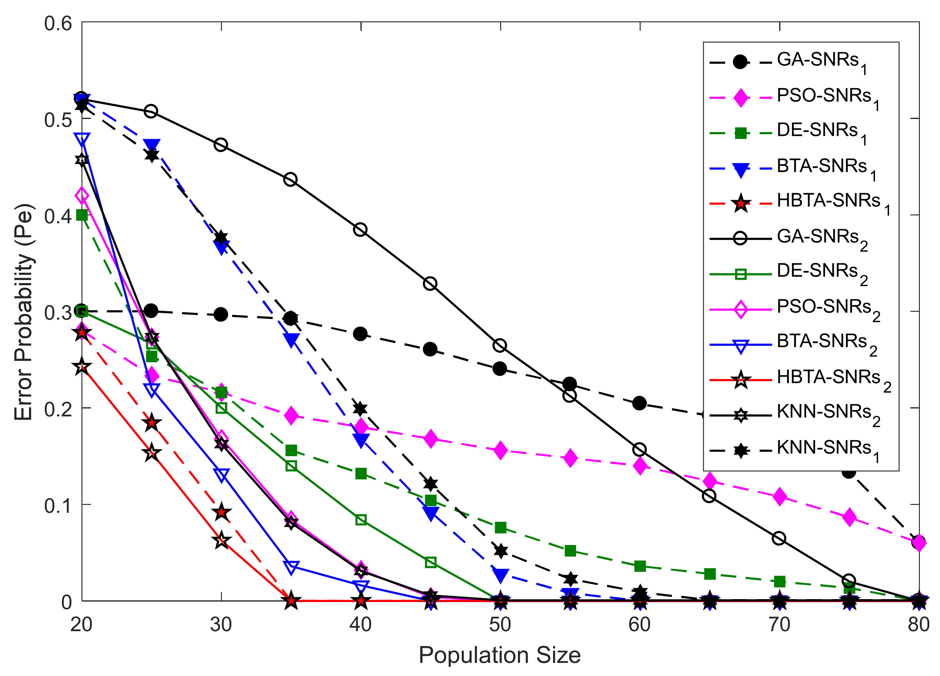
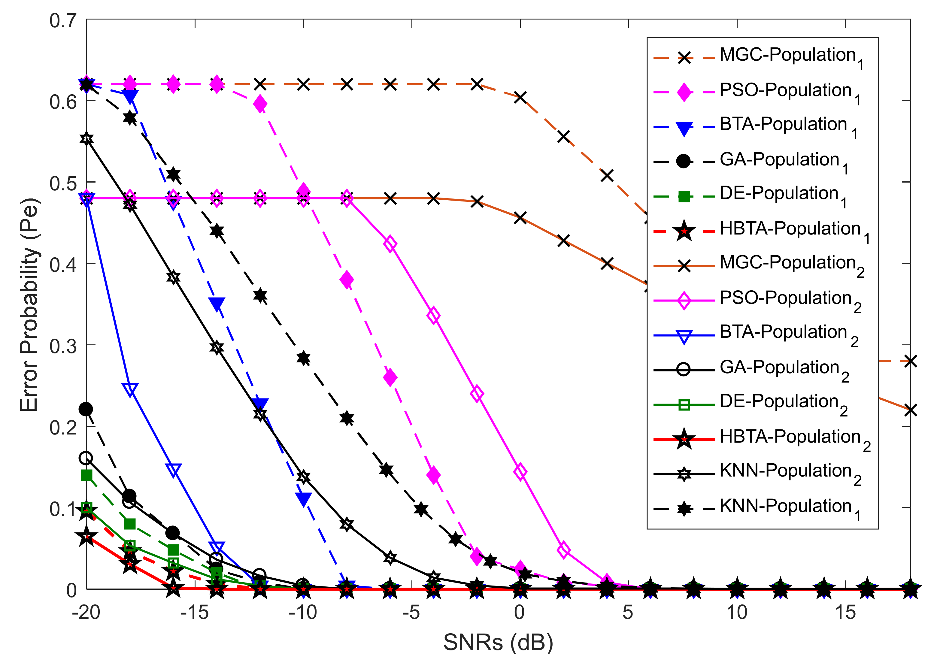
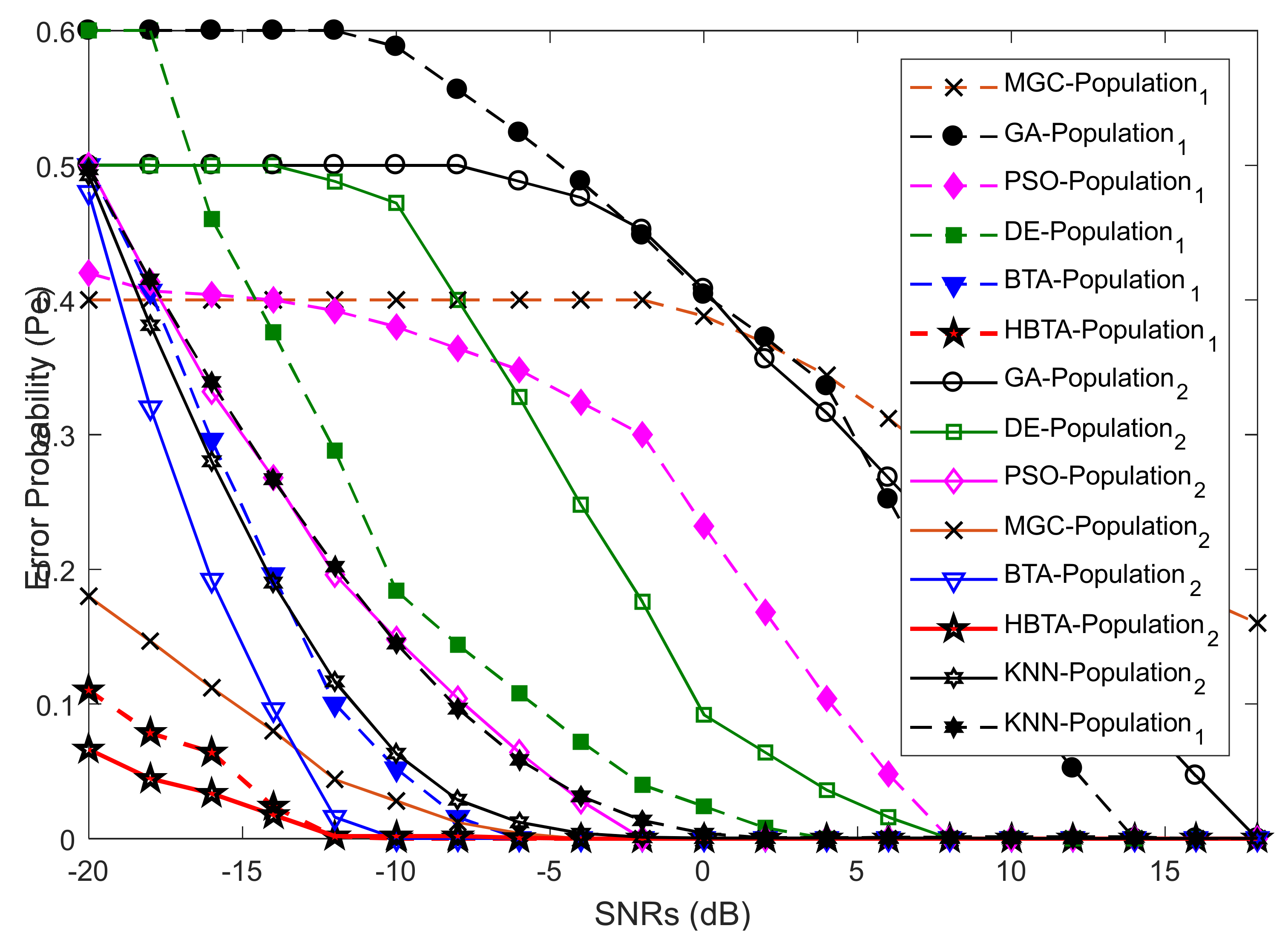
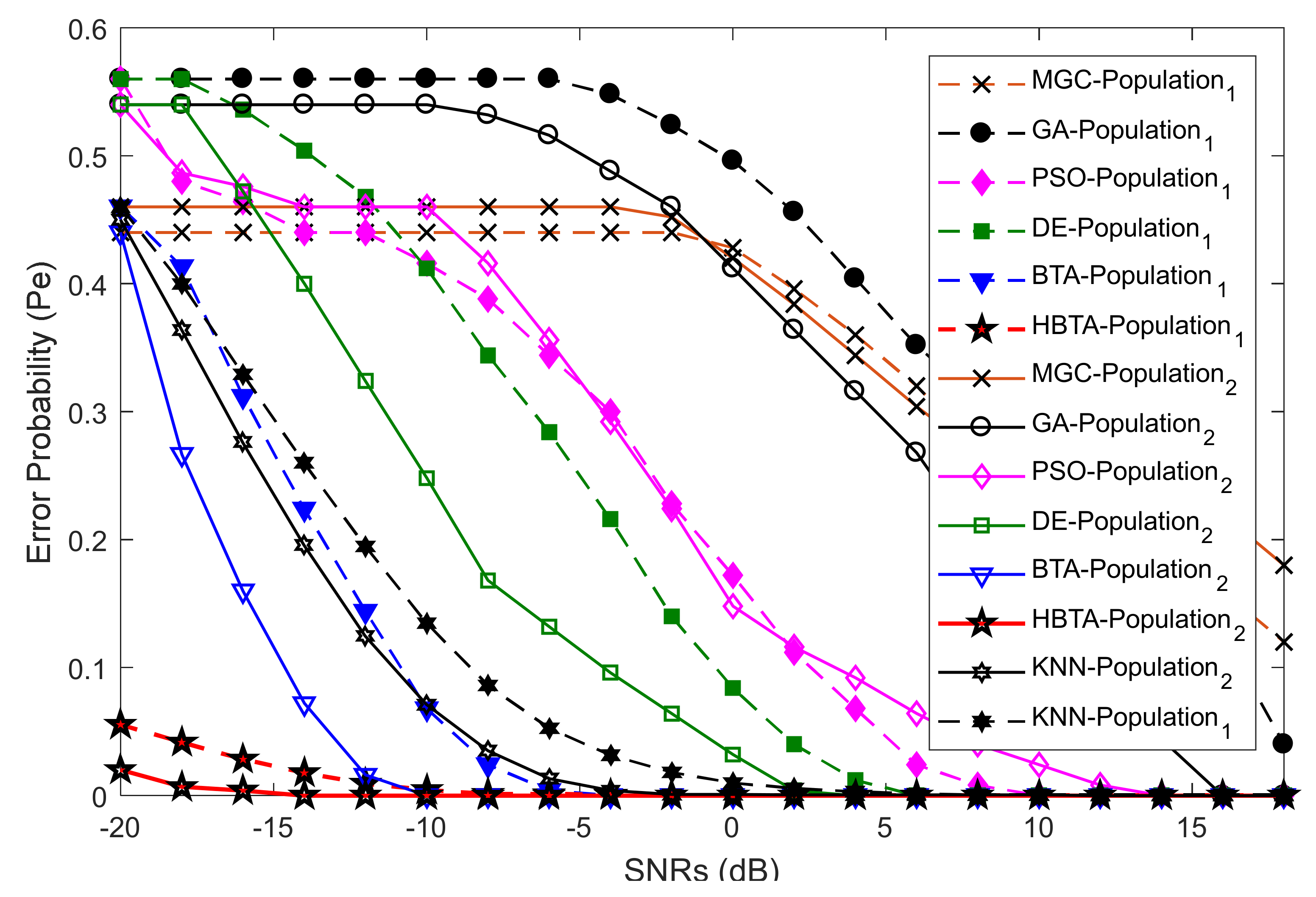
Case 2:

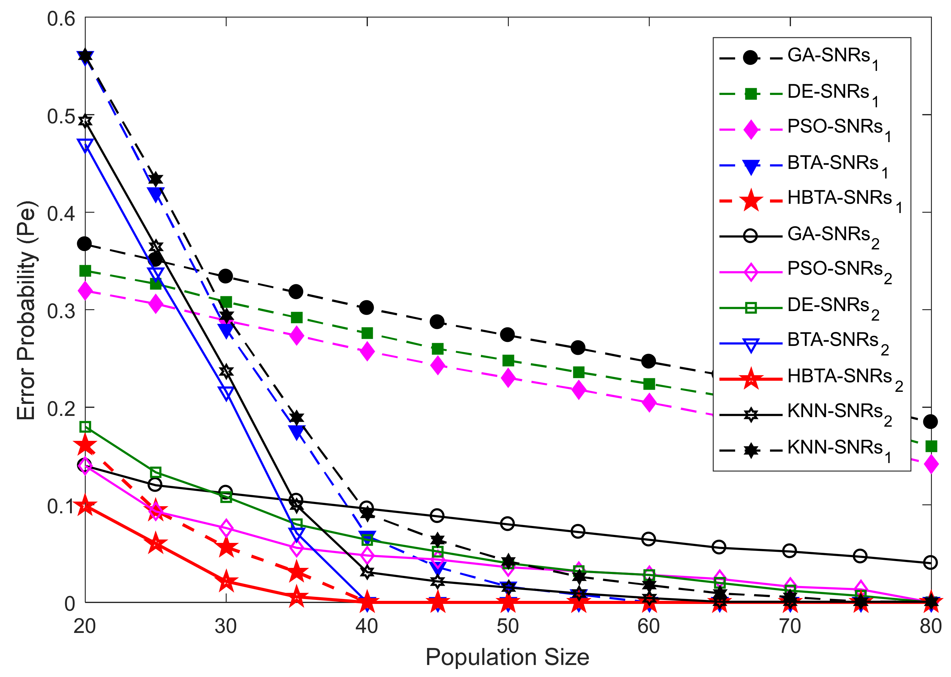
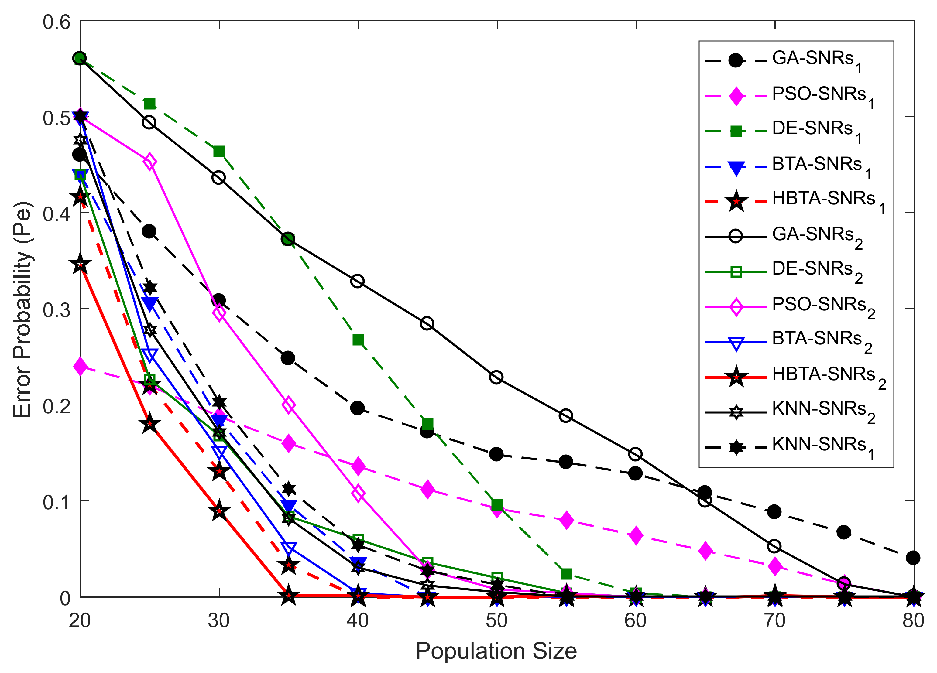
Case 2 showed the error probability results against varying population sizes of the optimization algorithms at two different SNR levels of −9.5 dB and −0.5 dB. Here, the total number of sensing iterations was kept at 50, with 270 sensing samples and a total number of 14 SUs. The error probability results collected against the FC’s decision with the contributions of AY-AYC, AN-ANC, and AO-AOC categories of MUs are shown in Figure 7, Figure 8 and Figure 9. The result in Figure 7 when the AY-AYC category of MUs participated in CSS shows better sensing performance for the proposed HBTA scheme with SNRs of both −9.5 dB and −0.5 dB. Similarly, the simple BTA and KNN schemes, as shown in the figure, were able to dominate PSO, DE, and GA schemes with minimum sensing, while the GA-based combination scheme was able to produce high sensing error at both SNR values. The results with the contribution of the AN-ANC category of MUs in CSS are illustrated in Figure 8. The results in Figure 8 show improved sensing results for the proposed HBTA scheme, followed by the results of the simple BTA and KNN schemes. The GA scheme in Figure 8 showed the worst sensing performance of all schemes. Finally, in Case 2, the performance of CSS was investigated with the participation of the AO-AOC category of MUs, which always negates the actual PU channel statistics. In Figure 9, the proposed HBTA scheme can be seen to show high sensing reliability with minimum sensing error as compared with all other schemes.

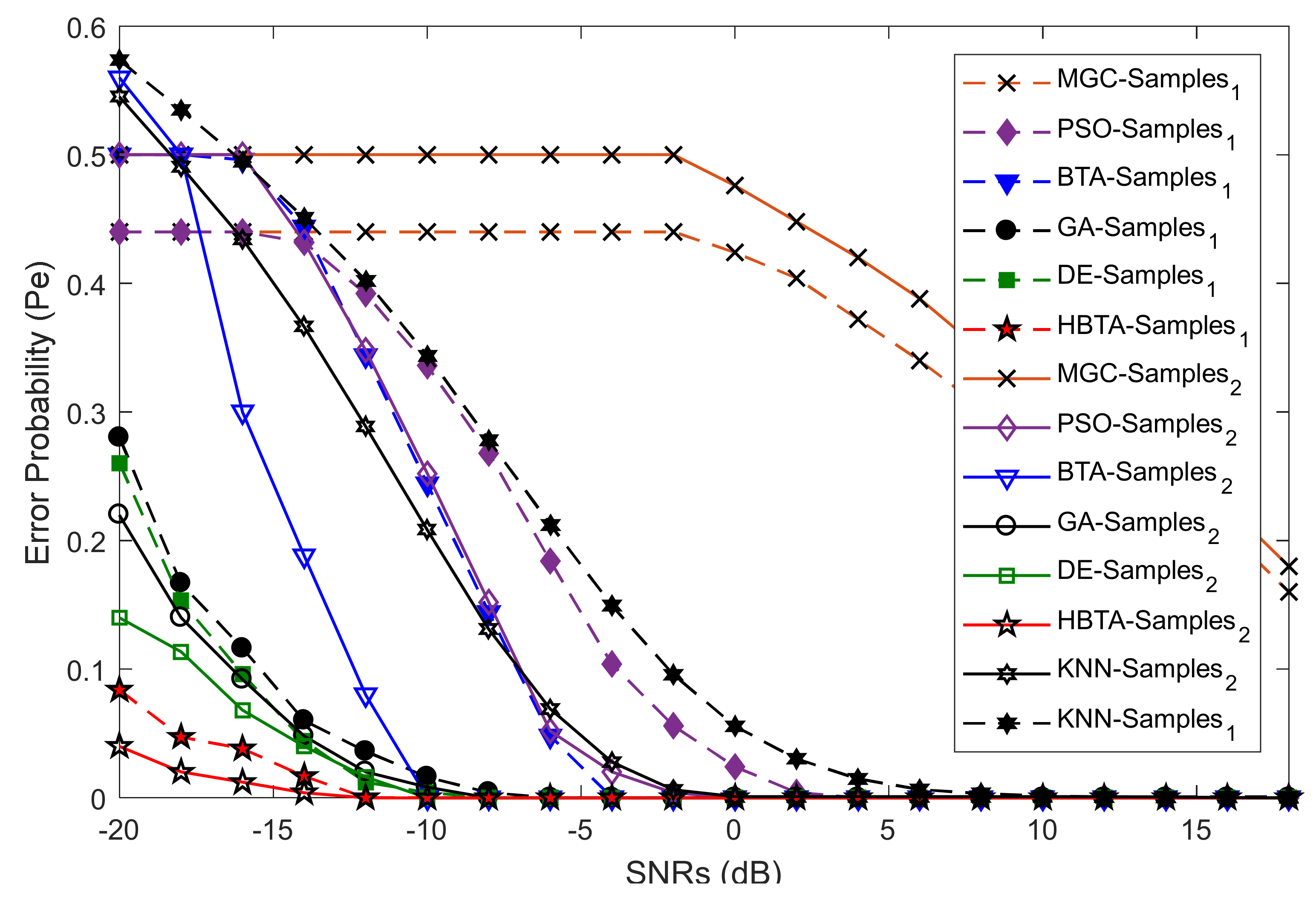
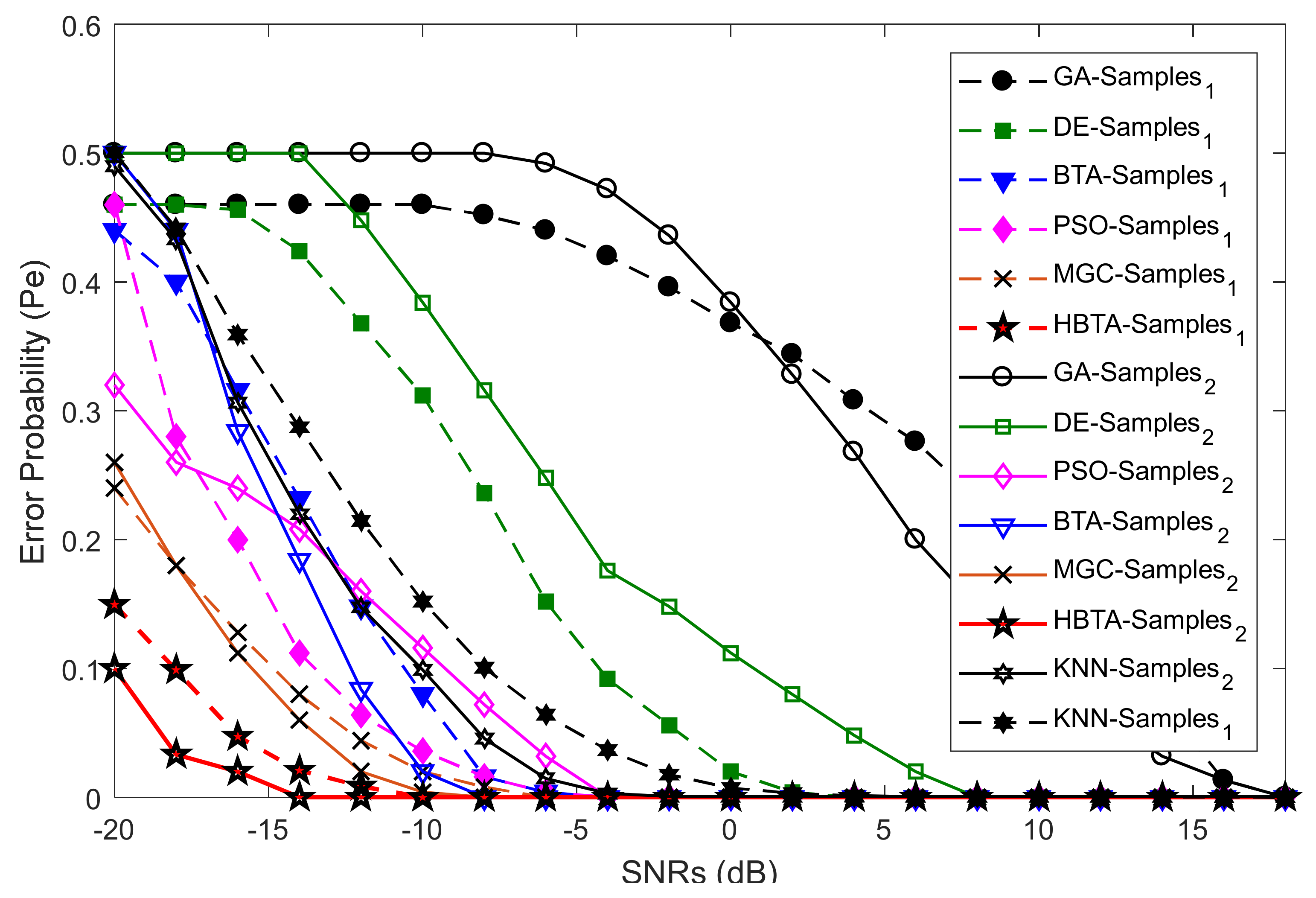
Case 3:

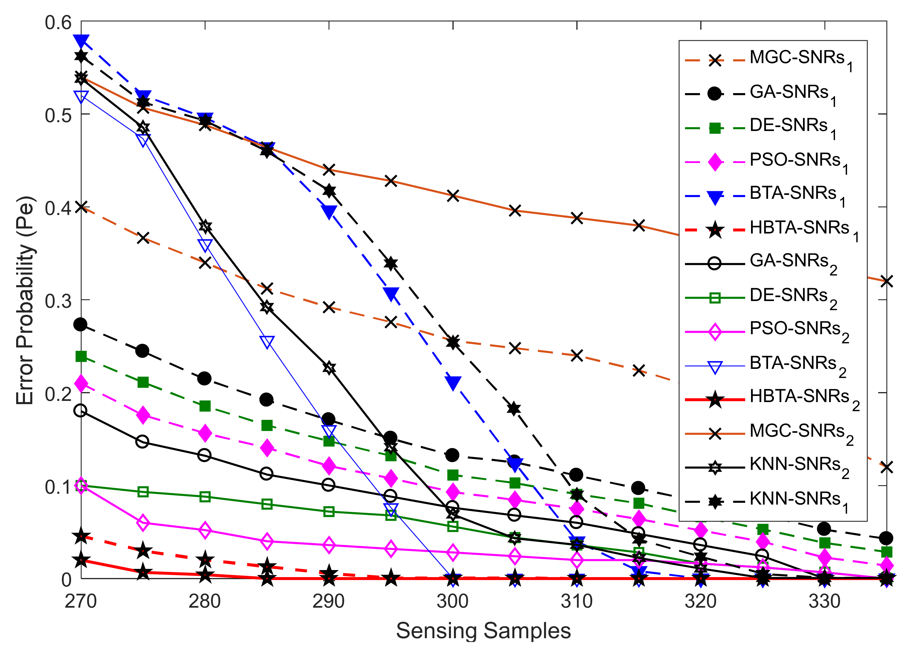
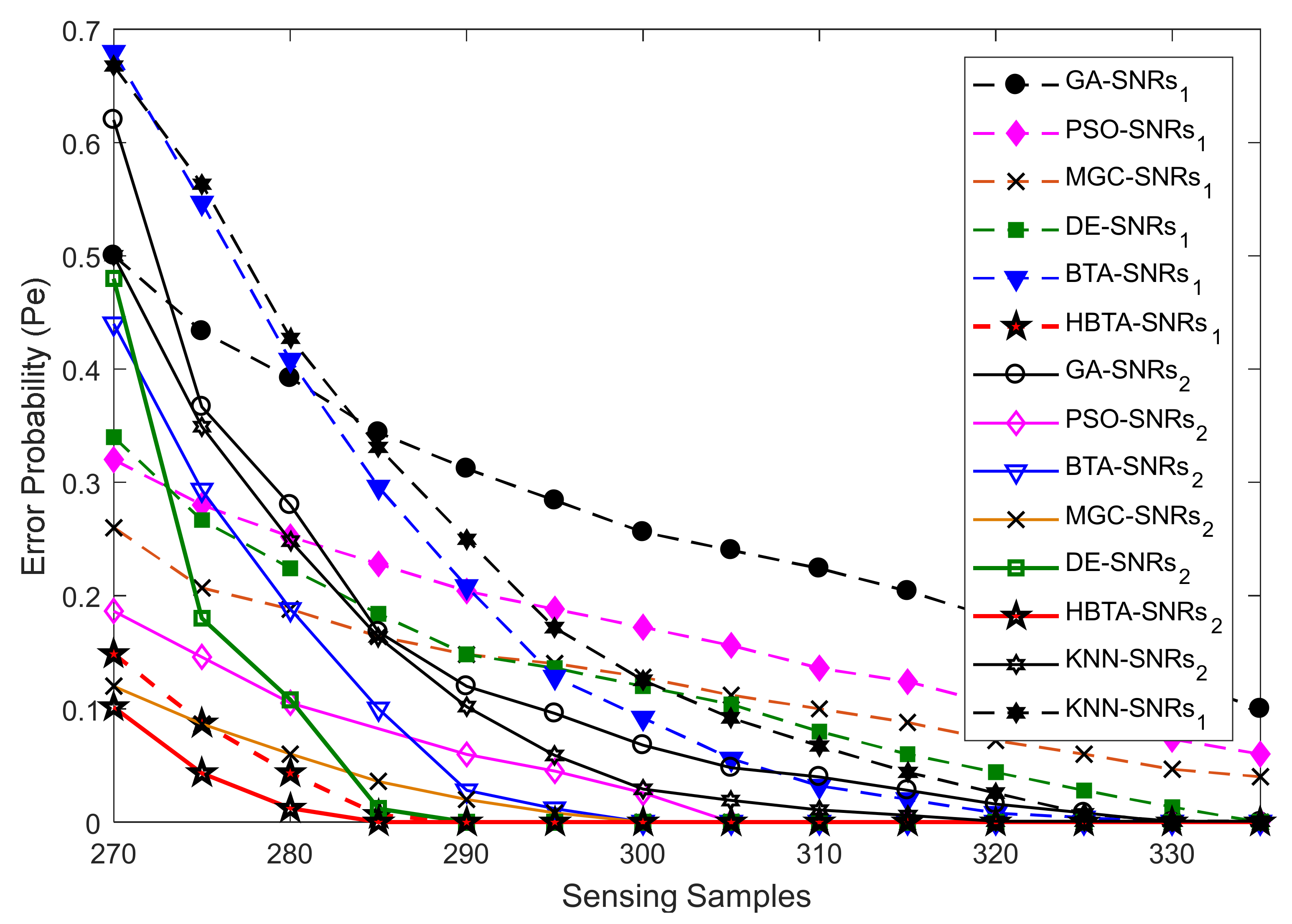
Case 3 explored the error probability results with varying sensing samples of the SUs at two different SNR values of −9.5 dB and −0.5 dB, as shown in Figure 10, Figure 11 and Figure 12. The total number of sensing iterations was kept at 50, the population size was 30, and the total number of SUs was 14. The AY-AYC, AN-ANC, and AO-AOC MUs were differently investigated in the simulation results. The result in Figure 10 shows that the proposed HBTA dominated all other schemes with all sensing sample values and both SNR levels. The proposed HBTA scheme’s results were followed by the simple BTA and KNN schemes, which had initially high sensing error results, but as the sensing sample increased, they could outperform the PSO, DE, GA, and MGC schemes. The result in Figure 11 shows the error probability results when the AN-ANC category of MUs participated in reporting their location decisions to the FC. Similarly, the DE combination scheme in this part could dominate the simple BTA, KNN, PSO, and GA combination schemes. The GA combination schemes in this part showed a high sensing error, leading to minimum sensing performance. Figure 12 shows the error probability results against increasing sensing samples at two different SNR values of −9.5 dB and −0.5 dB. The graphical results in the figure were collected with the presence of the AO-AOC category of MUs in CSS, with improved sensing performance shown by the proposed HBTA scheme in comparison with all other schemes, while the GA combination scheme can be seen to have exhibited the worst sensing reliability in Figure 12. Thus, it is concluded from the various graphical results in Case 2 that the proposed HBTA scheme has the best sensing reliability in producing improved sensing results as compared with the KNN, simple BTA, GA, PSO, and DE optimization schemes.

Case 4:

In this portion of the simulation results, error probabilities were collected with increasing SNR values at two different numbers of algorithm iterations: 60 and 85. Here, the SU sensing samples were fixed at 270 with an algorithm population size of 20 and total number of SUs of 14.

Figure 13 shows the error probability results of the proposed approach and all other schemes with the contribution of AY-AYC MUs. The results in Figure 13 show improved sensing results for the proposed HBTA scheme at both algorithm iteration levels. It is visible from the graphical illustrations that the DE-based combination scheme resulted in the best sensing decision with minimum sensing error in comparison with PSO, GA, KNN, and the simple BTA and MGC schemes, with the highest error probability results obtained for the MGC scheme. The results in Figure 14 show that AN-ANC user effects were strongly overwhelmed by the proposed scheme while making a global decision; therefore, the proposed HBTA scheme resulted in the minimum error probability results in comparison with all other schemes. In this part of the simulation, the simple BTA scheme was able to surpass the KNN, MGC, DE, PSO, and GA combination schemes when the SNRs were increased beyond certain limits, as shown in the figure. The GA scheme was able to reduce the error probability to a minimum by a sufficient increase in the SNR values. The proposed HBTA scheme was capable of keeping error probability at minimum with the contribution of AO-AOC users in Figure 15, in a similar manner to the AN-ANC users who participated in the CSS system.

Case 5:

Case 5 explored the error probability results against increasing SNR values with two different algorithm population sizes: 30 and 55. The total number of sensing samples for the SUs was selected as 270, with 50 algorithm iterations, as shown in Figure 16, Figure 17 and Figure 18. These results were investigated in the presence of AY-AYC, AN-ANC, and AO-AOC categories of MUs. In the first part of Case 4, the participation of AY was investigated in CSS to obtain the error probability results at different levels of SNRs. Figure 16 shows that satisfactory sensing results were achieved by the proposed HBTA, DE, and GA schemes. The simple MGC and PSO algorithm results were the worst of all investigated schemes. The results achieved with the contribution of AN-ANC users that always negate the actual states of the PU channel and result in constant channel availability are shown in Figure 17. The result shows the dominant performance of the proposed HBTA scheme. The third part of Case 5 explored the results obtained from the proposed and existing schemes with the AO-AOC category of MUs that negate the actual PU status by reporting high-energy states when a PU is absent and reporting low energy states when the PU is available in the given spectrum. The results in Figure 18 clarify the superiority of the proposed scheme to obtain a low sensing error at low levels of SNRs. It is also clear from the figure that simple BTA and KNN schemes performed better than the proposed scheme. The DE algorithm showed better sensing results in comparison with the PSO, GA, and MGC combination schemes. It is also visible from this part of the simulation results that the global decisions made using MGC and GA schemes exhibited minimum reliability with a high sensing error at both population levels.

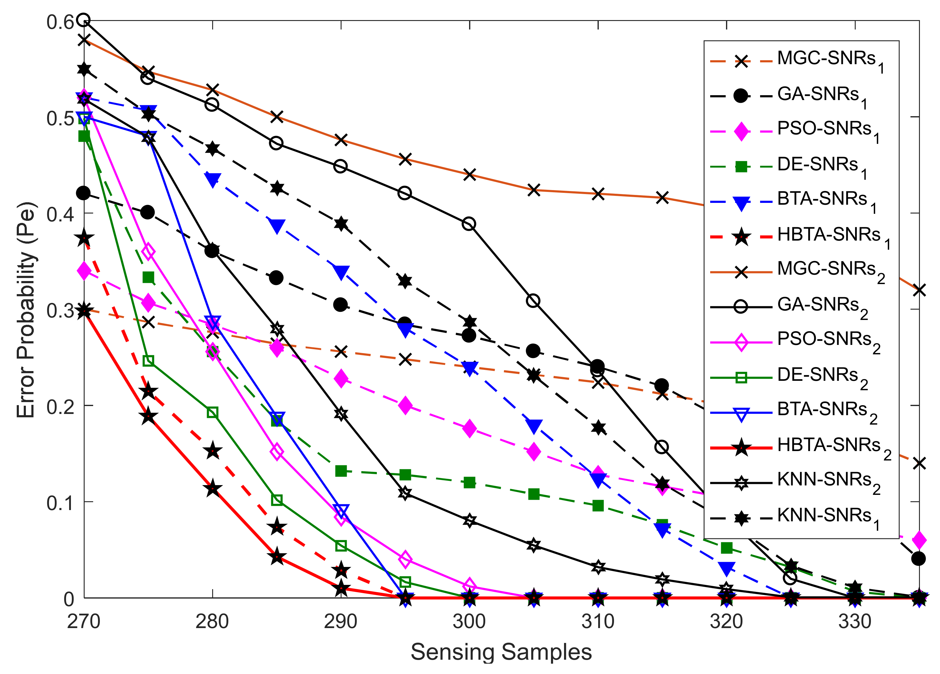
Case 6:

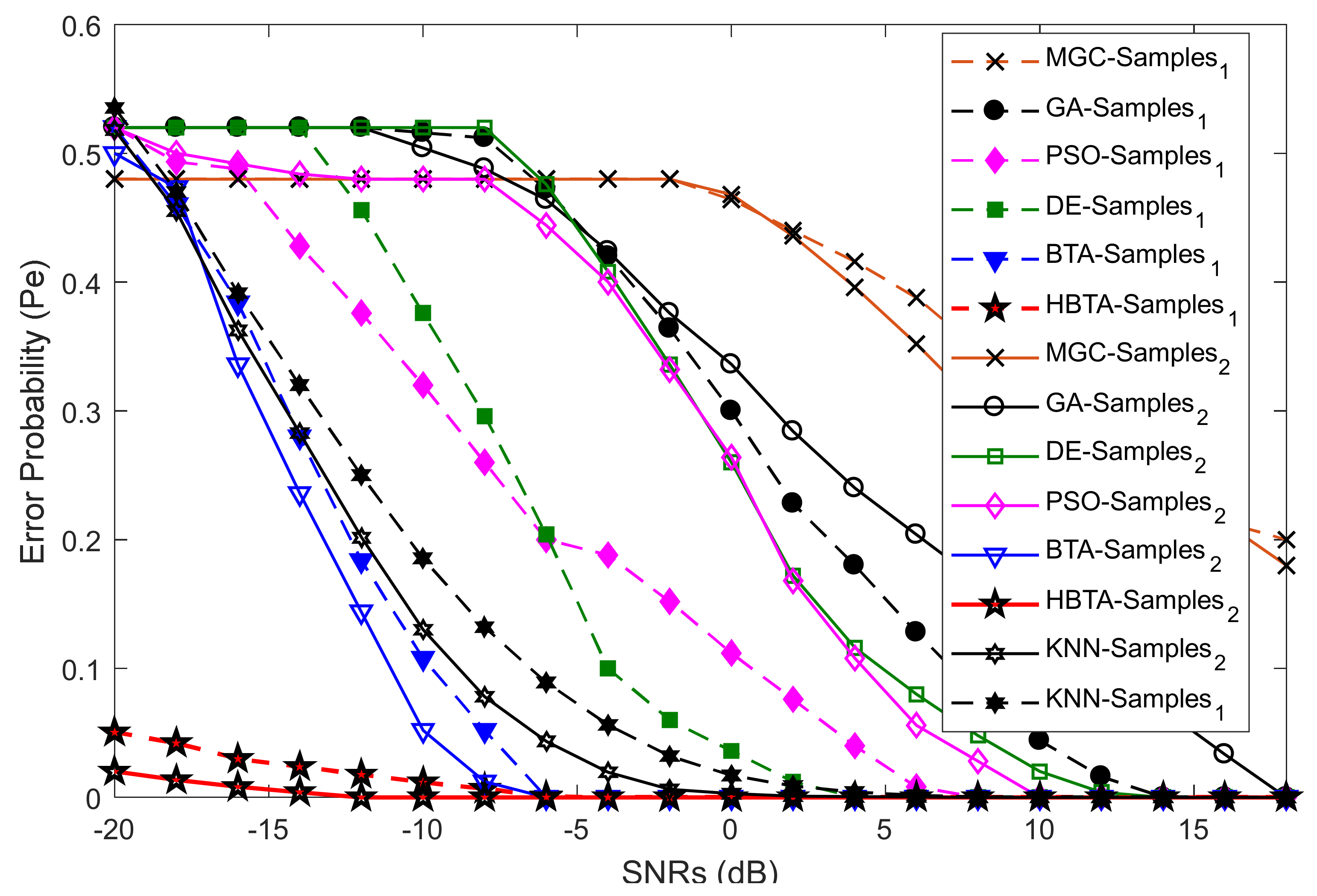
Finally, the error probability results were collected at varying SNRs, and two different levels of sensing samples were employed by the SUs: 280 and 305. To obtain the results, error probabilities were determined with the participation of AY-AYC, AN-ANC, and AO-AOC categories of Mus, as shown in Figure 19, Figure 20 and Figure 21. The error probability results in Figure 19 when AY-AYC participated in the CSS show improved sensing performance with low sensing error results for the proposed HBTA scheme. The result of the proposed HBTA scheme was followed by the DE and GA schemes, which showed improved sensing performance in comparison with the simple BTA, KNN, PSO and MGC schemes. The MGC scheme employed at the FC to make a global decision about the PU channel showed the highest sensing error of all schemes at different levels of SNRs. In the second part of Case 6, when AN-ANC users were allowed to participate in CSS, is shown in Figure 20. The figure shows that better sensing results with minimum sensing error were achieved by the proposed scheme in comparison with all other schemes. The MGC scheme results were reliable, producing minimum sensing error, as compared with the DE, PSO, and GA combination schemes. These results were followed by the simple BTA and KNN schemes, while the GA optimization scheme results were the worst of all schemes. In the third part of Case 6, the proposed HBTA scheme was compared with all other schemes with the participation of the AO-AOC category of MU. The proposed HBTA scheme in this part greatly outperformed all other schemes by producing minimum sensing error results. It is also clear from the results in Figure 21 that the simple BTA and KNN schemes in this part of the simulation showed improved sensing results as compared with GA, DE, PSO, and MGC combination schemes. Similarly, the MGC combination scheme was observed to have the worst sensing performance with the participation of the AO-AOC category of MUs.

5. Conclusions and Future Work

The sensing reliability of SUs leads to challenges in the Raleigh fading environment. The proposed hybrid scheme in this paper combines the DE optimization scheme with the ML-based BTA algorithm with the aim of augmenting the sensing performance of CSS. The simulation results were obtained considering a variety of MU categories in CSS. To evaluate the effectiveness of the proposed scheme, sensing error was evaluated for multiple cases based on variations in SNRs, algorithm iterations, algorithm population, and sensing samples in the presence of AY-AYC, AN-ANC, and AO-AOC. The results validate the superiority of the proposed HBTA scheme in comparison with several other existing schemes.

To extend this work in the future, we intend to compare the proposed HBTA scheme with deep learning algorithms, such as the recurrent neural network (RNN). Furthermore, we plan to reduce sensing costs by reducing the sensing time and energy consumption while utilizing ML and deep learning techniques.