Article

Forecasting of Photovoltaic Power by Means of Non-Linear Auto-Regressive Exogenous Artificial Neural Network and Time Series Analysis

by
Mohamed Louzazni
1,*,
Heba Mosalam
2,* and
Daniel Tudor Cotfas
3,*
1
Science Engineer Laboratory for Energy, National School of Applied Sciences, Chouaib Doukkali University, El Jadida 24000, Morocco
2
Electromechanics Department, Faculty of Engineering, Heliopolis University, Cairo 11785, Egypt
3
Department of Electronics and Computers, Transilvania University of Brasov, Eroilor 29, 500036 Brasov, Romania
*
Authors to whom correspondence should be addressed.
Submission received: 20 July 2021 / Revised: 10 August 2021 / Accepted: 11 August 2021 / Published: 13 August 2021
(This article belongs to the Special Issue Photovoltaic Energy Systems and Storage)

Abstract

:
In this research paper, a nonlinear autoregressive with exogenous input (NARX) model of the nonlinear system based on neural network and time series analysis is proposed to deal with the one-month forecast of the produced power from photovoltaic modules (PVM). The PVM is a monocrystalline cell with a rated production of 175 watts that is placed at Heliopolis University, Bilbéis city, Egypt. The NARX model is considered powerful enough to emulate the nonlinear dynamic state-space model. It is extensively performed to resolve a variety of problems and is mainly important in complex process control. Moreover, the NARX method is selected because of its quick learning and completion times, as well as high appropriateness, and is distinguished by advantageous dynamics and interference resistance. The neural network (NN) is trained and optimized with three algorithms, the Levenberg–Marquardt Algorithm (NARX-LMA), the Bayesian Regularization Algorithm (NARX-BRA) and the Scaled Conjugate Gradient Algorithm (NARX-SCGA), to attain the best performance. The forecasted results using the NARX method based on the three algorithms are compared with experimentally measured data. The NARX-LMA, NARX-BRA and NARX-SCGA models are validated using statistical criteria. In general, weather conditions have a significant impact on the execution and quality of the results.

1. Introduction

1.1. Background

Recently, forecasting renewable energy sources or solar radiation has become a major challenge for numerous researchers [1]. Forecasting photovoltaic temperature and power output and optimizing the injected power to the grid play vital roles in the smart grid and in the stability of the network. Moreover, supplying the network or isolated system with sufficient electricity can be key in a photovoltaic generator. It is important to analyze and study the performance of the injected power from the photovoltaic system to ensure the stability of the network. A photovoltaic panel has a non-linear and complex electrical equivalent circuit, which imposes serious instability in the generated power. Photovoltaic structures are essentially variable, unstable and are greatly affected and dependent on several factors, such as meteorological parameters, shading conditions, dust, sand and soiling deposition, wind speed and orientation and cable losses [2]. Any problems occurring on the photovoltaic panels, such as hot-spots, shading and dust, can be transferred to the grid, affecting the produced power output and also affecting the used inverter and converter. These instabilities and disturbances can be transferred to the network and influence its stability. In order to inject stable power to ensure the stability of the network, forecasting of a photovoltaic system will be necessary for monitoring the consumption of the power system [3]. In this instance, a number of studies have proposed various strategies and methods to forecast several parameters in a photovoltaic system. The selected technique depends mainly on different parameters and available data, which depend on weather conditions [4,5]. It is classified into (i) very short-term, (ii) short-term, (iii) medium-term and (iv) long-term forecasting.
The existing forecasting methods and techniques can be classified into physical methods, statistical methods and hybrid methods. The physical methods are mostly dependent on meteorological variables that influence electricity generation. These methods are mainly based on mathematical equations, which use several parameters to transform solar radiation into electricity. The above models can be simple and depend on sunlight, or they can be complex and include further parameters such as ambient temperature, soiling, cable losses and humidity [6]. The statistical modeling techniques are supported by data that have been tested for repeatability and reproduced at periodic intervals [7]. They are based on previous experimental data that have been analyzed by applying time-series data and measured parameters correlated with meteorological information based on the assumption that historical data will reappear in the future [8]. Hybrid methods are a combination of the aforementioned methods [9]. The objectives are to combine several techniques to overcome the limitations of a simple technique and to improve the outcomes’ effectiveness.

1.2. Literature Review

In the research literature, numerous papers predicting the generated output power of photovoltaic systems have been published, applying different techniques and methods. An artificial neural network (ANN) calibration methodology has been used to forecast the day-ahead of photovoltaic power in Milan, Italy [10]. The approach was used to determine the optimum network settings in terms of layer number, neurons and trials. The results were validated by using different statistical indexes, particularly the normalized mean absolute error (NMAE%), with low values. Another study used a Radial Belief Neural Network (RBNN) to forecast power generated by large photovoltaic plants in India [11]. The performance of the RBNN was compared with deep and machine learning techniques in terms of the different statistical indexes. The results showed that the RBNN generates low errors compared with the other techniques. The Internet of Things (IoT) was implemented to collect different natural factors in the environment to forecast the generated energy from a photovoltaic module using ANN [12]. The technique reduced the mean square error (MSE) while improving the forecasting effectiveness. The investigation, on the other hand, failed to offer the necessary data for appropriate model training. This resulted in the inability to train ANNs adequately due to the lack of some crucial features. A combination of the WRF-solar model with multi-layered urban canopy and building energy models was utilized to provide an integrated physical approach. A fuzzy c-means optimized by Whale Optimization Algorithm (WOA) and Least Squares Support Vector Machine (LSSVM) were used to forecast the day ahead for a photovoltaic power station with 2.2 MW capacity [13]. The results showed that the forecasting accuracy using WOA-LSSVM outperformed LSSVM, long short-term memory (LSTM), and Particle Swarm Optimization-Backpropagation (PSO-BP) in terms of root mean square error (RMSE) under different climatic conditions. A hybrid model combining Wavelet Transform (WT), PSO and support vector machines (SVMs) was implemented to forecast short-term photovoltaic power [14]. The results using the WT-PSO-SVM outperformed seven different models, namely a Back Propagation Neural Network (BPNN), Hybrid Genetic Algorithm and Neural Network (HPNN), SVM, Hybrid Genetic Algorithm (HGS), hybrid PSO–SVM and Hybrid Hilbert–Huang Transform (HHT). On the other hand, a Moth Flame Optimization Algorithm (MFOA) was proposed to optimize the SVM parameters in order to forecast the photovoltaic power output [15]. This methodology led to enhanced forecasting accuracy, according to the conclusions. These investigators primarily used classical optimization approaches to achieve the forecasting performance of SVM by optimizing the parameter values. The optimized genetic algorithm has been proposed to optimize Bidirectional Long Short-Term memory (BiLSTM) to forecast multiple photovoltaic power outputs [16]. The results demonstrate the importance of adjacent photovoltaic system power series, and the suggested model performs adequately in ultra-short-term forecasting.
The acquisition of photovoltaic power data has stationary points, and to overcome this problem, a statistical method has been developed for the short-term (0–6 h) forecasting of the power output of a photovoltaic system [17]. The paper presented a forecasting methodology that uses existing data from geographically distributed photovoltaic installations to forecast the power production of a given plant by exploiting spatial and temporal correlations. These approaches were investigated by analyzing the relationship between historical performance and the associated meteorological data. The method used a network of sensors made up of geographically scattered power plants. The used input was derived from the prepared data and not based on the global solar irradiation data, and the Numerical Weather Predictions (NWP) were not taken into consideration. In relation to state-of-the-art forecasting methodologies, the Normalized Root Mean Square Error (nRMSE) can be reduced by 20% or more. Again, for short-term forecasting of the power output of a photovoltaic system, a new probabilistic method has been proposed based on a competitive ensemble of diverse base predictors [18]. The author selected three different probabilistic methods and trained them as base predictors in order to construct an ensemble of the predictive distribution with the best precision and accuracy criteria. These methods have been implemented in three different steps to form a probabilistic multi-model ensemble forecast. In terms of production forecast dependability, the Multi-Objective (MO) optimization technique outperformed the Single-Objective (SO) optimization technique by a wide margin, with minimal Continuous Ranked Probability Score (CRPS) losses. A simple forecasting model was compared with more complicated and sophisticated models over 32 photovoltaic plants of different sizes and technology over a period of one year [19]. The collected data were classified into three categories, namely meteorological data, measured data and computed data. The data were trained hourly, and the results were evaluated using different performance indices; the normalized Mean Absolute Error (nMAE) was the main index compared with other algorithms. The accuracy and quality of the results were evaluated using the Grey Box (GB) model, Quantile Random Forest (QRF) and an ensemble of methods. The results were improved by 5% in terms of nMAE. In another paper, the output power of a photovoltaic system was forecasted using a hybrid Deep Learning (DL) system based on Convolutional Neural Networks (CNN) and Long-Short Term Memory Recurrent Neural Networks (LSTM) [20]. The CNN model was used to find nonlinear patterns and persistent frameworks in prior output power data, allowing for a more accurate photovoltaic power forecast. The LSTM was also used to estimate the photovoltaic power of the following time step by modeling the dynamic variations in the previous photovoltaic data. The suggested approach was thoroughly tested on data from a photovoltaic system installed in Limberg, Belgium, and numerical results show that it can deliver good photovoltaic system predictive accuracy.
Recently, the NARX technique monthly based on NN and time-series analysis have been widely used in several papers to solve nonlinear and complex systems. This technique has already proven its immense potential through its capability to forecast complicated input–output correlations, and it has become a significant aspect of the modern approach to forecasting [21]. To reduce the computational costs associated with the linearity in the variable’s mode, the NARX model is sometimes described as a continuous combination of complex functions [22]. NARX structures are well-suited to learning approaches, and their composition is complicated by the fact that the number of terms is rapidly increasing. The NARX methodology is generally recognized as a powerful modeling and evaluation technique that converges slightly quicker and generalizes far more than most other NN methodologies. These were created to handle time-dependent operating conditions using real-time data from equipment activity. Because the validity of the results is simple to compute and the prediction results are simple to interpret, NARX was widely used to handle a range of data-driven modeling difficulties. Generally, the purpose of the NARX method is to predict the next power output using the time-series y(t) based on the identification of the previous information of the same exogenous information and previous information of the time-series x(t) [23].

1.3. Contributions

The aim of this paper is to consider the application of the NARX model combined with NNs and time-series to predict the power of photovoltaic modules for one month. The PVM system is installed on the rooftop of Heliopolis University on the eastern edge of the southern Nile delta in Egypt. It is located on the east side of the Nile, with coordinates given as Latitude = 30.420 and Longitude = 31.565. The used data are collected from the monocrystalline modules with 175 W peak solar power fabricated by SunModule SW linked to a converter (Sunny Island) [24]. The above PVM is investigated in [25], which has indicated that the monocrystalline PVM is the best equipment for a hot climate after studying the influence of the experimental module on power generation. The proposed method uses solar radiation, hours and temperature as the exogenous variables. The NARX paradigm is assumed to be capable of simulating a highly nonlinear state-space model. It is also widely used to handle a range of issues, and it is mainly important in sophisticated control applications. The NARX model is also chosen because of its quick training and convergence times, as well as its exceptional accuracy and attractive dynamics and interference tolerance. In this paper, three algorithms are used to train and improve the NNs: NARX-LMA, NARX-BRA and NARX-SCGA. In order to evaluate the quality of the results, a comparison between the experimental measurement is presented. For further accuracy, the statistical measures are generated to examine the efficacy and productivity of the NARX-LMA, NARX-BRA and NARX-SCGA models. The results show that NARX-BRA outperforms NARX-LMA and NARX-SCGA in terms of Mean Absolute Error (MAE), Mean Absolute Percentage Error (MAPE), Residual Sum of Squares (RSSE), Root Mean Squared Error (RMSE), Auto-Correlation Function (ACF) and R2. Finally, the results reveal that the NARX-BRA models are suitable for performing the one-month time-series composite index forecasting.
This paper is organized as follows: in Section 2, we provide a description and a presentation of the photovoltaic system, weather characteristics and the used methodologies. Section 3 deals with the forecasting performance metrics. Section 4 illustrates the simulation, presents a comparison of the results and provides an assessment of the prediction accuracy measures, as well as the discussion, and Section 5 concludes this study.

2. Materials and Methods

This section presents the implementation of the NARX model to forecast the power output of the PVM system. The PVM is installed in Heliopolis University, Belbeis city, Egypt. The system is installed to supply electricity to the university, which is connected to the grid. A weather station collects various data daily, such as solar radiation, ambient temperature and the power output of the photovoltaic modules. The output power is forecasted using the NARX model based on neural network time-series and the NARX-LMA, NARX-BRA and NARX-SCGA optimized training algorithms.

2.1. Photovoltaic Module and Weather Station

The photovoltaic modules are SunModule SW monocrystalline cells with 175 W peak solar power, located on the Nile’s southern delta, with coordinates La = 30.420 and Lo = 31.565. The modules are fabricated by Solar Word, with an innovative module structure. They are made up of 72 series-connected cells with 125×125 mm dimensions and a generation capacity of 4.5 kWp. The electrical characteristics of the monocrystalline photovoltaic modules at STC are Pmax = 175 Wp, Vmpp = 35.7, Impp = 4.9 A, Voc = 44.4 V and Isc = 5.4 A [26]. The PVM is coupled to an SMA inverter and is inclined at a predefined angle to collect the maximum power throughout the day. Figure 1 illustrates the photovoltaic modules on the roof-top of the university [27].
In this investigation, the monocrystalline PV (Figure 1) was chosen for the aforementioned purposes:
(1)
this is the most commonly used device in Egypt;
(2)
it has the most reasonable costs among its competitors;
(3)
according to manufacturer reports, it has the best heat resistance.
Numerous papers have analyzed the performance of the 175 W SunModule SW monocrystalline cell. The thermal effects are reported in [28] by using different microinverter placements. It indicates that, at lower temperatures, the performance is approximately reduced by 0.65%, while the AC/power is enhanced by 0.9%. The electrical characteristics and performance analyses are provided in [29]. The supervision and control of the used PVM linked to two stages and connected to a DC/DC converter at the string level and the main inverter are presented in [30]. Another publication discusses and presents the experimental analysis and investigation of the single-phase Z-source inverter attached to the used photovoltaic modules (175 W SunModule SW monocrystalline) [31].

2.2. NARX Neural Network Model

The NARX neural network technique is an important class of nonlinear recurrent dynamic ANN computer program networks comprising linked nodes inspired by a simplification of the human neural system. As a result, every point contains an artificial neuron that takes one or more inputs and accumulates them and passes through a non-linear active function to generate an output [32,33,34,35]. In the Feedforward Neural Networks (FNNs) model, the information moves in one direction, with nodes structured in layers. Meanwhile, in a Recurrent Neural Network (RNN) architecture, such as NARX, the information/communication moves both forward and backward, providing connections between neurons situated in the same or previous layers [36]. This structure evaluates the present level of an incoming time-series with preceding values of the same series, as well as the present and previous values of an exogenous series. This typically includes simulating the inputs and outputs of complex processes, constructed by two tapping delays, one flowing over the inputs and the other over the outputs. Likewise, the NARX methodology takes time-series data and is based on the linear autoregressive exogenous (ARX) model. The NARX technique is indeed an important form of discrete-time of a nonlinear system. The time-series y(t) can be presented as the weighted sum of n independent power outputs of a photovoltaic system presented by P 1 ( t ) ,   P 2 ( t ) ,   P n ( t ) as [22,37]:
y ( t ) = a 0 + a 1 P 1 ( t ) + a 2 P 2 ( t ) + + a n P n ( t ) + e ( t )
where e(t) is the deviation error.
The new value of y(t) is directly reliant on the previous output parameters and even the previous independent exogenous input parameters when a NN multilayer perceptron predicts the function f.
y ( t ) = [ P 1 ( d 1 ( t ) ) P 2 ( d 2 ( t ) ) , , P 31 ( d 31 ( t ) ) ]
where d i ( t ) ,   ( i = 1 , 2 , 31 ) is the days of each power given as
d ( t ) = [ d 1 ( t ) d 2 ( t ) , , d 31 ( t ) ]
Nonlinear multidimensional equations could be approached using a linear structure of nonlinear functions, and the function f can be modeled as follows:
f [ P ] = f [ P 1 , P 2 , , P n ] = a 0 + f 1 ( P 1 ) + f 2 ( P 2 ) + , , f n ( P n ) + e ( t )
The input u(t) and output y(t) of a nonlinear model are modeled and approached by:
y ( t ) = a 0 + i = 1 n a a i y ( t i ) + j = 1 n b b j u ( t j ) + e ( t )
The values of a 1 , a 2 , a n a and b 1 , b 2 , b n a are constant, the system exponent number is na, and nb represents the input exponent number.
Generally, the function f is nonlinear, and the future values of y(t) are extrapolated on prior output and input u(t) values. The desired forecasted values of the power output generated by the photovoltaic system are regressed by direct feedback and connected with the output and input of the multi-layer NN. Figure 2 gives a description of the input and output in the NARX model’s NN framework [38].
The nonlinear function f has a multilayer perception and consists of different nodes structured in two layers; the first layer is named H and performs the output function, and Z represents the second layer, which refers to the value of a node’s activation. In complete NNs, the activation function and system parameters have always been associated one to one and aggregated. The value of the state variables is estimated by the next step and can be modeled as follows:
x i ( t + 1 ) = z i ( t )
The weight and number of each node are external inputs in the NARX architecture model, while the activation function for each node is presented as:
z ( t ) = f [ w 0 + j = 1 i = 1 , , H m a i j x j ( t ) + b i u ( t ) + c i ]
The real values of the weights a i j , b i and c i are fixed, and the output layer y(t) is made up of a single linear node, written as:
y ( t ) = w 0 + i = 1 H w i j z i ( t ) + e ( t )

2.3. Levenberg–Marquardt Training Algorithm

The LMA is an adaptable and flexible methodology that interpolates between the Gauss–Newton algorithm (GNA) and the Gradient-Descent Method (GDM) [39] to identify a multidimensional function’s lowest values [40]. As evidenced by many applications, the LMA is more trustworthy than the GNA, and it may identify a solution even when starting from a very low point [41]. The LMA uses the GDM to initialize the variables of the model in the contrary direction of the gradient of the objective function if the first assumption of the variable’s type is not enough to reach their optimal point. The minimal element is calculated as the sum of squares from nonlinear real-valued functions [42]. If the initial estimate is around or close to the optimum, the LMA selects the GNA by supposing that the objective function is quadratic [43].
If LMA uses a sum of squares as an objective function using the Hessian matrix, and considering the mathematical equation of LMA as a linear approximation of the function f, the LMA can be formulated as [44]:
{ H = J . J x k + 1 = x k [ J . J + μ I ] 1 . J . ε
where J indicates the Jacobian matrix, x k + 1 the Hessian matrix, xk represents the weight vector, µ represents the scalar operator, I is the identity matrix, and ε represents the residual error vector.

2.4. Bayesian Regularization Training Algorithm

The BRA is recognized to be one of the best methods for handling NN learning problems since it can randomly select regularization coefficients and combines the high-convergence qualities of traditional BP with earlier Bayesian statistics [45]. Regularization is a training method that significantly enhances the recognition accuracy by incorporating a limitation notion into the NN’s training criterion component in order to ensure that the network’s weight connection is properly configured [46]. The supplementary term is written in the following form:
{ F = β E d + α E w E w = 1 2 i = 1 n w i 2
where ED and Ew are the sum of squared network errors and the sum of squared network weights, respectively. While α and β denote the regularization parameters [47], their values can be determined by:
{ α = γ 2 E w β = M γ 2 E d γ = n 2 α . t r ( H ) 1 H = β 2 E d + α 2 E w
where γ is the effective weight and H is the Hessian matrix of the objective function.

2.5. Scaled Conjugate Gradient Training Algorithm

The SCGA technique is a set of fundamental approaches for reducing smooth functions, particularly when the dimension is largely based on conjugate directions [48]. In SCGA, the gradient is simply implemented to define the first error descent direction, which we can indicate by D(0), and then each successive direction is considered to be congruent with the preceding one, i.e., for those along which there is something, the gradient varies only in magnitude rather than direction [49]. This was created to eliminate the time-consuming process of searching for boundaries. After this, a line search mechanism is utilized to reduce the error function. In MATLAB, ‘trainscg’ is a network training function that uses the Scaled Conjugate Gradient (SGG) methodology to adjust weights and biases [50]. This could train a certain network that has derivative functions for the weight, net-input and transfer functions. This algorithm can be summarized in five steps, by supposing that the beginning point for the local optimization operation is w(0) [51,52]:
Step 1: k = 0 and the error value in w(0) is generated from gradient vector [53]
{ e ( 0 ) = E [ w ( 0 ) ] g ( 0 ) = E [ w ( 0 ) ]
Step 2: if k modd = 0, then
D ( k ) = g ( k )
Otherwise,
D ( k ) = g ( k ) + λ D ( k 1 )
The coefficient λ determines how many of the previous search directions are included in the present one. This could be any of a variety of different formulations. In our investigation, we used the one proposed by Polak and Ribiere, which is more reliable in non-quadratic error functions, which, according to [54], and presented in the following equation:
λ = [ g ( k ) ] T [ g ( k ) g ( k 1 ) ] [ g ( k ) ] T g ( k 1 )
Step 3: To find a step size φ, execute a line search, starting at w(k) and moving through the directions D(k), that is close enough to the minimum of the set of variable functions given by:
F ( φ ) = E [ w ( k ) + φ D ( k ) ]
Step 4: This step deals with the adjustment of the approximated minimum of E, and it could be given by:
w ( k + 1 ) = w ( k ) + φ D ( k )
Step 5: k = k + 1
{ e ( k ) = E [ w ( k ) ] g ( k ) = E [ w ( k ) ]
If the termination criteria are not met, move to Step 1.
It is indeed noticeable that the line adopted in the proposed algorithm has a considerable impact on the algorithm’s general performance.

3. Forecasting Performance Metrics
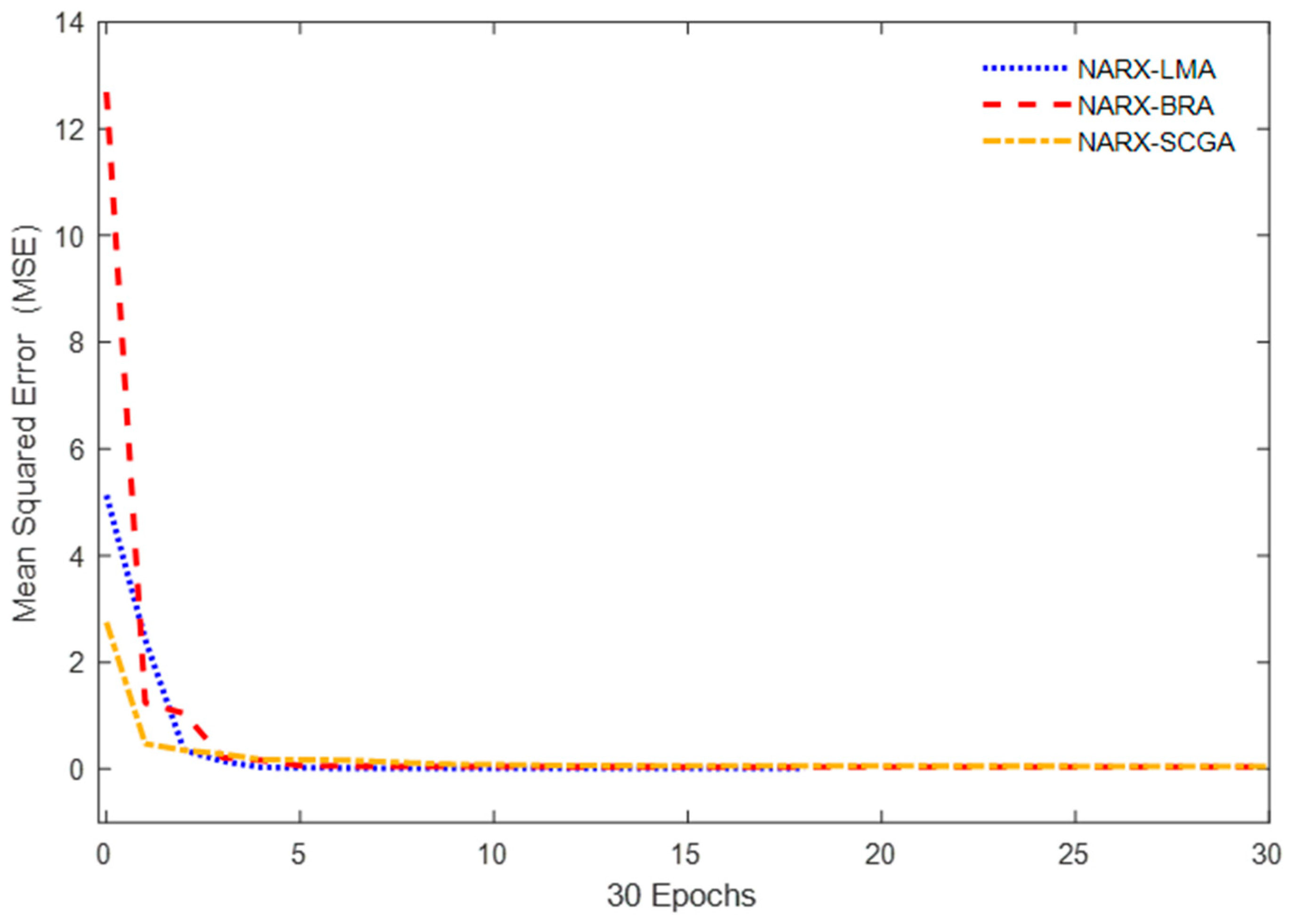
To evaluate and verify the efficiency and correctness of the proposed forecasting models, experimental data from the PVM system in Heliopolis university are used. Various statistical criteria are adopted and used to measure the forecast accuracy [55]. The statistical criteria are applied in a wide range of scientific disciplines to properly evaluate the suitability of a forecasting model [56]. These statistical criteria are typically determined by the difference between the experimental power Pexp and the forecast power Pfor, referred to as the t-th time’s sample. The approximated models are evaluated based on a comparison of statistical criteria to maintain the quality and effectiveness of the results.
The Individual Error (IE) is commonly used and defined as the difference between the experimental and forecasted power.
I E = P exp , i P for , i
Starting from the IE, the other error indexes adopted for the assessment can be derived:
Relative Error (RE):
R E = P exp , i P for , i P exp , i
Mean Absolute Error (MAE):
M A E = 1 N i = 1 N | P exp , i P for , i |
Mean Absolute Percentage Error (MAPE):
M A P E = 100 N i = 1 N | P exp , i P for , i | P exp , i
Residual Sum of Squares (RSSE):
R S S E = i = 1 N ( P exp , i P for , i ) 2
Mean squared error (MSE):
M S E = 1 N i = 1 N ( P exp , i P for , i ) 2
Root Mean Squared Error (RMSE):
R M S E = 1 N i = 1 N ( P exp , i P for , i ) 2
Coefficient of Determination: The R2 was used to examine the appropriate following explanation among both observed and predicted values [57], and it was written as:
R 2 = 1 i = 1 m ( P exp , i P for , i ) 2 i = 1 m P exp , i 2 i = 1 m P for , i 2 m
where N is the number of measured powers.
The autocorrelation function (ACF) indicates how and why the correlation among any given input values varies when their separation changes. For the error signal, the ACF can be presented as:
A C F = C o n v ( e t , e t + k ) V a r ( e t ) V a r ( e t + k )

4. Results

In this section, the forecasting models used are implemented by using measured data from the 175 W peak photovoltaic modules, installed at the roof-top of the Heliopolis University for Sustainable Development, Belbeis city, Egypt. The PVMs are monocrystalline, with 72 cells linked in series. The used exogenous daily experimental data are measured during the daytime and heavily depend on the weather conditions. Figure 3a shows a comparison of the specific inverter total yield by kWh of the injected power by the PVM for January, February and March of 2018.
The system experiences several natural problems, such as raining or soiling, which can increase the generated power energy production from the photovoltaic modules. For example, Figure 3b presents the soiling in the PVM due to wind, rain and sand. The fluctuation in power production illustrated in Figure 3a is due to the soiling caused by wind, rain and sand, because the system is installed in the desert. Köppen–Geiger categorizes the site as being in Egypt’s hot desert, with warm and long summers; winters are damp, sandy and cold, and the atmosphere is mostly clear. Throughout the year, the temperature regularly ranges between 10 and 36 °C, with temperatures rarely falling below 7 °C or rising over 39 °C [58]. To illustrate and forecast the power output of the PVM, we considered daily measured data for one month. The experimental data are measured every hour during August and the former 450 sampling points considered are the input data for the NARX model.
The performance, quality and accuracy of the proposed models are compared using 10 and 6 numbers of input hidden neurons with 1, 2 and 3 delayers for the one-day pass as time delays. In order to forecast the next day’s energy P(t) given previous at d day of P(t + 1) and a different series x(t), the configuration of the NARX approach is illustrated in Figure 4 [38].
Generally, the NARX model is based on the following three time-stage targets:
  • The network is trained and its deviation is corrected;
  • Validation is used to check the adaptation of the network and to avoid training from increasing the generalization of the network;
  • Testing with low impact on training, as well as providing independent network output analysis before and after training.
The NARX model is implemented, designed and trained in open-loop form, to rectify the previous training inputs that were supposed to obtain the correct outputs of the current loop. Table 1 highlights the forecasted output power effectiveness for the three training algorithms.
The index metrics R2 are calculated to assess the efficiency of the predicted results compared to the experimental results. The R2 quantifies the correlation among predicted and measured values in the interval [0 1]; there is no positive correlation if it equals zero, or if it is one, it indicates that the connection is excellent. Generally, the low values of MSE and the high value of R2 imply good training, and the forecasted values could be near to the experimental values.
From Table 1, the value and high value of MSE and R2 can be obtained for the NARX-BRA. Figure 5 shows the compared performance of NARX-LMA, NARX-BRA and NARX-SCGA in terms of MSE.
Figure 6 depicts a regression plot of the difference among both forecasted measured and forecasted values. The best value of R2 = 0.9927 is obtained for NARX-BRA, which is close to 1.
Figure 6 illustrates the measured power output of the PVM compared with the forecasted power using NARX-LMA, NARX-BRA and NARX-SCGA for the seven and six days. Applying 10 and 6 hidden layers, and 1 and 3 delays, the performance and accuracy of the employed NARX models are evaluated.
Figure 7 presents the obtained results using the three optimization training algorithms, which are close to the measured power output of the PVM.
From Figure 8, all the evaluated results are similar, and it is difficult to determine which training algorithm is more effective and performs faster. In order to compare the performance of the NARX-LMA, NARX-BRA and NARX-SCGA and present each algorithm more accurately, the IE and RE with 6 hidden layers and 3 time delays are presented and compared in Figure 8.
The effectiveness of the evaluated optimization training algorithms is determined using statistical criteria. The IE indicates the systematic errors, whereas the RE provides the measurement precision. The IE presents the quantity of quantitative inaccuracy and is the difference between the experimentally measured power and the forecasted power using the three optimization training algorithms.
The RE is considered an accuracy indicator and is the fraction of a measurement’s IE to the measuring being taken. In other words, this form of error is proportional to the size of the object being measured. Figure 9 presents a comparison of IE and RE using the three selected techniques, indicating that the NARX-LMA and NARX BRA present low values for IE and RE. For more precision, we need to calculate another statistical index to further determine the best optimization training algorithm.
The autocorrelation function (ACF) describes how and why the correlation among any consecutive signal values varies as their dispersion varies. It is a time-domain measure of stochastic process memory that provides no information about the framework’s frequency content.
Figure 10 depicts the ACF test, which clarifies that the forecasted output power of the PVM using NARX-LMA, NARX-BRA and NARX-SCGA validates the test, as the values are in the range of −1 and 1.
Table 2 presents a comparison between different performance metrics for the three used training optimization algorithms. The aim is to determine the best NARX model in terms of the forecasting power output of the PVM. The lowest values of the statistical error index illustrate the best forecasting data.
The NARX-BRA showed the lowest statistical metric values for IAE, MAE, MAPE, SSE, RMSE and R2 values compared with NARX-LMA and NARX-SCGA. It can be concluded that the NARX-BRA is able to forecast the power output produced by the PVM.

5. Conclusions

This paper presents the one-month forecasting of the generated power from photovoltaic modules installed in a hot area in Egypt at the Nile delta. The monocrystalline photovoltaic modules are connected to the grid of Heliopolis University. A NARX approach is presented and used to overcome several problems that can occur during the forecasting. It was selected for its power to forecast various fields, and it is an ensemble of a neural network and time-series analysis. The NARX model was chosen due to its high flexibility of use and ability to train a nonlinear model with an input–output relationship utilizing time data.
The neural network of the NARX was trained using three algorithms, namely the Levenberg–Marquardt Algorithm, Bayesian Regularization Algorithm and Scaled Conjugate Gradient Algorithm, to attain the best performance using experimental data collected daily during the hot month of August 2018. The theoretical results obtained using the three training algorithms were compared with the experimental power data. In order to enhance the validity of the method used, various statistical indexes were calculated to compare the accuracy, quality and performance of the results. In this paper, the NARX-BRA showed the lowest values for MAE = 0.0030, MAPE = 7.8334 × 10⁻⁶, RSSE = 8.9073 × 10⁻⁶, RMSE = 1.981 × 10⁻² and R2 = 0.99271. NARX-BRA outperformed the NARX-LMA and NARX-SCGA. The NARX model can forecast the power of a photovoltaic system under different conditions, such as ambient temperature, wind speed and solar radiation in humid and hot regions. The effectiveness and correctness of the results are, in general, highly influenced by the environment and data inputs.
Future research may address the forecasting of short-term photovoltaic module temperature and solar radiation using NARX and other optimization training algorithms. This method can also be applied for the forecasting of hybrid systems in terms of predicting the self-consumption of a photovoltaic/battery/supercapacitor system.

Author Contributions

Conceptualization, M.L.; methodology, M.L.; software, M.L; validation, M.L.; formal analysis, M.L.; investigation, M.L.; resources, H.M.; data curation, M.L. and H.M.; writing—original draft preparation, M.L. and H.M.; writing—review and editing, M.L., H.M. and D.T.C.; visualization, M.L. and H.M.; supervision, M.L.; funding acquisition, D.T.C. All authors have read and agreed to the published version of the manuscript.

Funding

This research received no external funding.

Data Availability Statement

The data are available on request to Heba Mosalam.

Acknowledgments

The authors would like to acknowledge the “Energy Department of Heliopolis University for Sustainable Development”, Cairo, Egypt for providing the experimental data for this research. M. Louzazni and D.T Cotfas are highly grateful to the “Romanian Ministry of Foreign Affairs” and the “Agence Universitaire de la Francophonie” for the “Eugen Ionescu” mobility grant from the “Transilvania University of Brasov”, Brasov, Romania.

Conflicts of Interest

The authors declare no conflict of interest.

References

  1. Wang, Y.; Wu, L. On practical challenges of decomposition-based hybrid forecasting algorithms for wind speed and solar irradiation. Energy 2016, 112, 208–220. [Google Scholar] [CrossRef] [Green Version]
  2. Hosseini, S.A.; Kermani, A.M.; Arabhosseini, A. Experimental study of the dew formation effect on the performance of photovoltaic modules. Renew. Energy 2019, 130, 352–359. [Google Scholar] [CrossRef]
  3. Babatunde, A.A.; Abbasoglu, S. Predictive analysis of photovoltaic plants specific yield with the implementation of multiple linear regression tool. Environ. Prog. Sustain. Energy 2019, 38, 13098. [Google Scholar] [CrossRef]
  4. Sobri, S.; Koohi-Kamali, S.; Rahim, N.A. Solar photovoltaic generation forecasting methods: A review. Energy Convers. Manag. 2018, 156, 535–576. [Google Scholar] [CrossRef]
  5. Kleissl, J. Solar Energy Forecasting and Resource Assessment; Academic Press: Cambridge, MA, USA, 2013. [Google Scholar]
  6. Monteiro, C.; Fernandez-Jimenez, L.A.; Ramirez-Rosado, I.J.; Muñoz-Jimenez, A.; Lara-Santillan, P.M. Short-Term Forecasting Models for Photovoltaic Plants: Analytical versus Soft-Computing Techniques. Math. Probl. Eng. 2013, 2013, 767284. [Google Scholar] [CrossRef] [Green Version]
  7. Montgomery, D.C.; Jennings, C.L.; Kulahci, M. Introduction to Time Series Analysis and Forecasting; John Wiley & Sons: Hoboken, NJ, USA, 2015; Chapter 2; p. 25. [Google Scholar]
  8. Rouchier, S.; Rabouille, M.; Oberlé, P. Calibration of simplified building energy models for parameter estimation and forecasting: Stochastic versus deterministic modeling. Build. Environ. 2018, 134, 181–190. [Google Scholar] [CrossRef]
  9. Ferlito, S.; Adinolfi, G.; Graditi, G. Comparative analysis of data-driven methods online and offline trained to the forecasting of grid-connected photovoltaic plant production. Appl. Energy 2017, 205, 116–129. [Google Scholar] [CrossRef]
  10. Grimaccia, F.; Leva, S.; Mussetta, M.; Ogliari, E. ANN Sizing Procedure for the Day-Ahead Output Power Forecast of a PV Plant. Appl. Sci. 2017, 7, 622. [Google Scholar] [CrossRef] [Green Version]
  11. Natarajan, Y.; Kannan, S.; Selvaraj, C.; Mohanty, S.N. Forecasting energy generation in large photovoltaic plants using radial belief neural network. Sustain. Comput. Inform. Syst. 2021, 31, 100578. [Google Scholar]
  12. Barrera, J.M.; Reina, A.; Maté, A.; Trujillo, J.C. Solar energy prediction model based on artificial neural networks and open data. Sustainability 2020, 12, 6915. [Google Scholar] [CrossRef]
  13. Gu, B.; Shen, H.; Lei, X.; Hu, H.; Liu, X. Forecasting and uncertainty analysis of day-ahead photovoltaic power using a novel forecasting method. Appl. Energy 2021, 299, 117291. [Google Scholar] [CrossRef]
  14. Eseye, A.T.; Zhang, J.; Zheng, D. Short-term photovoltaic solar power forecasting using a hybrid Wavelet-PSO-SVM model based on SCADA and Meteorological information. Renew. Energy 2018, 118, 357–367. [Google Scholar] [CrossRef]
  15. Lin, G.Q.; Li, L.L.; Tseng, M.L.; Liu, H.M.; Yuan, D.D.; Tan, R.R. An improved moth-flame optimization algorithm for support vector machine prediction of photovoltaic power generation. J. Clean. Prod. 2020, 253, 119966. [Google Scholar] [CrossRef]
  16. Zhen, H.; Niu, D.; Wang, K.; Shi, Y.; Ji, Z.; Xu, X. Photovoltaic power forecasting based on GA improved Bi-LSTM in microgrid without meteorological information. Energy 2021, 231, 120908. [Google Scholar] [CrossRef]
  17. Agoua, X.G.; Girard, R.; Kariniotakis, G. Short-Term Spatio-Temporal Forecasting of Photovoltaic Power Production. IEEE Trans. Sustain. Energy 2018, 2, 538–546. [Google Scholar] [CrossRef] [Green Version]
  18. Bracale, A.; Carpinelli, G.; De Falco, P. A Probabilistic Competitive Ensemble Method for Short-Term Photovoltaic Power Forecasting. IEEE Trans. Sustain. Energy 2017, 8, 551–560. [Google Scholar] [CrossRef]
  19. Gigoni, L.; Betti, A.; Crisostomi, E.; Franco, A.; Tucci, M.; Bizzarri, F.; Mucci, D. Day-Ahead Hourly Forecasting of Power Generation from Photovoltaic Plants. IEEE Trans. Sustain. Energy 2018, 9, 831–842. [Google Scholar] [CrossRef] [Green Version]
  20. Li, G.; Xie, S.; Wang, B.; Xin, J.; Li, Y.; Du, S. Photovoltaic Power Forecasting with a Hybrid Deep Learning Approach. IEEE Access 2020, 8, 175871–175880. [Google Scholar] [CrossRef]
  21. Cheng, Y.; Wang, L.; Yu, M.; Hu, J. An efficient identification scheme for a nonlinear polynomial NARX model. Artif. Life Robot. 2011, 16, 70–73. [Google Scholar] [CrossRef]
  22. Haddad, S.; Mellit, A.; Benghanem, M.; Daffallah, K.O. NARX-Based Short-Term Forecasting of Water Flow Rate of a Photovoltaic Pumping System: A Case Study. J. Sol. Energy Eng. 2015, 138, 11004–11006. [Google Scholar] [CrossRef]
  23. Cococcioni, M.; D’Andrea, E.; Lazzerini, B. One day-ahead forecasting of energy production in solar photovoltaic installations: An empirical study. Intell. Decis. Technol. 2012, 6, 197–210. [Google Scholar] [CrossRef]
  24. SolarWorld Module SW 175 Monocrystalline. Available online: https://pdf.wholesalesolar.com/module%20pdf%20fold (accessed on 30 May 2021).
  25. Mosalam, H.A. Experimental investigation of temperature effect on PV monocrystalline module. Int. J. Renew. Energy Res. 2018, 8, 365–373. [Google Scholar]
  26. Buy Solar Module SolarWorld Sunmodule Plus SW 175 Mono | pvXchange.co. Available online: https://www.pvxchange.com/Solar-Modules/SolarWorld/Sunmodule-plus-SW-175-mono_1-2100535 (accessed on 23 May 2021).
  27. Louzazni, M.; Mosalam, H.; Khouya, A.; Amechnoue, K. A non-linear auto-regressive exogenous method to forecast the photovoltaic power output. Sustain. Energy Technol. Assess. 2020, 38, 100670. [Google Scholar] [CrossRef]
  28. Day, N.U.; Reinhart, C.C.; DeBow, S.; Smith, M.K.; Sailor, D.J.; Johansson, E.; Wamser, C.C. Thermal effects of microinverter placement on the performance of silicon photovoltaics. Sol. Energy 2016, 125, 444–452. [Google Scholar] [CrossRef]
  29. Alistoun, W.J. Investigation of the Performance of Photovoltaic Systems; Faculty of Science at the Nelson Mandela Metropolitan: Gqeberha, South Africa, 2012. [Google Scholar]
  30. Nichols, S.; Huang, J.; Ilic, M.; Casey, L.; Prestero, M. Two-stage PV Power System with Improved Throughput and Utility Control Capability. In Proceedings of the 2010 IEEE Conference on Innovative Technologies for an Efficient and Reliable Electricity Supply, Waltham, MA, USA, 27–29 September 2010; pp. 110–115. [Google Scholar]
  31. Rajakaruna, S. Experimental studies on a novel single-phase Z-Source inverter for grid connection of renewable energy sources. In Proceedings of the 2008 Australasian Universities Power Engineering Conference, Sydney, NSW, Australia, 14–17 December 2008; pp. 1–6. [Google Scholar]
  32. Di Nunno, F.; de Marinis, G.; Gargano, R.; Granata, F. Tide Prediction in the Venice Lagoon Using Nonlinear Autoregressive Exogenous (NARX) Neural Network. Water 2021, 13, 1173. [Google Scholar] [CrossRef]
  33. Buevich, A.; Sergeev, A.; Shichkin, A.; Baglaeva, E. A two-step combined algorithm based on NARX neural network and the subsequent prediction of the residues improves prediction accuracy of the greenhouse gases concentrations. Neural Comput. Appl. Mar. 2021, 33, 1547–1557. [Google Scholar] [CrossRef]
  34. Liu, Q.; Chen, W.; Hu, H.; Zhu, Q.; Xie, Z. An Optimal NARX Neural Network Identification Model for a Magnetorheological Damper with Force-Distortion Behavior. Front. Mater. 2020, 7, 10. [Google Scholar] [CrossRef]
  35. Ezzeldin, R.; Hatata, A. Application of NARX neural network model for discharge prediction through lateral orifices. Alex. Eng. J. 2018, 57, 2991–2998. [Google Scholar] [CrossRef]
  36. Chatterjee, S.; Nigam, S.; Singh, J.B.; Upadhyaya, L.N. Software fault prediction using Nonlinear Autoregressive with eXogenous Inputs (NARX) network. Appl. Intell. 2012, 37, 121–129. [Google Scholar] [CrossRef]
  37. Billings, S.A. Nonlinear System Identification: NARMAX Methods in the Time, Frequency, and Spatio–Temporal Domains; John Wiley & Sons: Hoboken, NJ, USA, 2013. [Google Scholar]
  38. Mathworks. Design Time Series NARX Feedback Neural Networks. 2019. Available online: https://ch.mathworks.com/help/deeplearning/ug/design-time-series-narx-feedback-neural-networks.html;jsessionid=38db5ec344dedde7319d3c0a7dbd (accessed on 30 May 2021).
  39. Koofigar, H.R. Adaptive robust maximum power point tracking control for perturbed photovoltaic systems with output voltage estimation. ISA Trans. 2016, 60, 285–293. [Google Scholar] [CrossRef] [Green Version]
  40. Adamowski, J.; Chan, H.F. A wavelet neural network conjunction model for groundwater level forecasting. J. Hydrol. 2011, 407, 28–40. [Google Scholar] [CrossRef]
  41. Levenberg, K. A Method for the Solution of Certain Problems in Least Squares. Quart. Appl. Math. 1944, 2, 164–168. [Google Scholar] [CrossRef] [Green Version]
  42. Brown, K.M.; Dennis, J.E. Derivative free analogues of the Levenberg-Marquardt and Gauss algorithms for nonlinear least squares approximation. Numer. Math. 1971, 18, 289–297. [Google Scholar] [CrossRef]
  43. Nocedal, J.; Wright, S.J. Numerical Optimization; Springer Science + Business Media, LLC: Berlin/Heidelberg, Germany, 2006. [Google Scholar]
  44. Kelley, C. Iterative Methods for Optimization; Society for Industrial and Applied Mathematics: Philadelphia, PA, USA, 1999. [Google Scholar]
  45. Sun, Z.; Chen, Y.; Li, X.; Qin, X.; Wang, H. A Bayesian regularized artificial neural network for adaptive optics forecasting. Opt. Commun. 2017, 382, 19–527. [Google Scholar] [CrossRef]
  46. Liu, J.; Zhao, L.; Mao, Y. Bayesian regularized NAR neural network based short-term prediction method of water consumption. E3S Web Conf. 2019, 118, 03024. [Google Scholar] [CrossRef]
  47. Louzazni, M.; Mosalam, H. Dailly Forecasting of Photovoltaic Power Using Non-Linear Auto-Regressive Exogenous Method. In Proceedings of the 2020 International Conference on Decision Aid Sciences and Application, DASA 2020, Online, 8–9 November 2020. [Google Scholar]
  48. Bandurski, K.; Kwedlo, W. A lamarckian hybrid of differential evolution and conjugate gradients for neural network training. Neural Process. Lett. 2010, 32, 31–44. [Google Scholar] [CrossRef]
  49. Cetişli, B.; Barkana, A. Speeding up the scaled conjugate gradient algorithm and its application in neuro-fuzzy classifier training. Soft Comput. 2010, 14, 365–378. [Google Scholar] [CrossRef]
  50. Babani, L.; Jadhav, S.; Chaudhari, B. Scaled conjugate gradient based adaptive ANN control for SVM-DTC induction motor drive. IFIP Adv. Inf. Commun. Technol. 2016, 475, 384–395. [Google Scholar]
  51. Møller, M.F. A scaled conjugate gradient algorithm for fast supervised learning. Neural Netw. 1993, 6, 525–533. [Google Scholar] [CrossRef]
  52. Feijóo, M.C.; Zambrano, Y.; Vidal, Y.; Tutivén, C. Unsupervised Damage Detection for Offshore Jacket Wind Turbine Foundations Based on an Autoencoder Neural Network. Sensors 2021, 21, 3333. [Google Scholar] [CrossRef]
  53. Arora, J.S. Optimum Design Concepts. In Introduction to Optimum Design; Elsevier: Amsterdam, The Netherlands, 2004; pp. 83–174. [Google Scholar]
  54. Richard, D.G.S.; Duda, O.; Hart, P.E. Pattern Classification, 2nd ed.; Wiley: New York, NY, USA, 2000. [Google Scholar]
  55. Louzazni, M.; Khouya, A.; Amechnoue, K.; Mussetta, M.; Crăciunescu, A. Comparison and evaluation of statistical criteria in the solar cell and photovoltaic module parameters’ extraction. Int. J. Ambient Energy 2020, 41, 482–1494. [Google Scholar] [CrossRef]
  56. Nespoli, A.; Ogliari, E.; Leva, S.; Massi Pavan, A.; Mellit, A.; Lughi, V.; Dolara, A. Day-Ahead Photovoltaic Forecasting: A Comparison of the Most Effective Techniques. Energies 2019, 12, 1621. [Google Scholar] [CrossRef] [Green Version]
  57. Kong, Y.S.; Abdullah, S.; Schramm, D.; Omar, M.Z.; Haris, S.M. Development of multiple linear regression-based models for fatigue life evaluation of automotive coil springs. Mech. Syst. Signal Process. 2019, 118, 675–695. [Google Scholar] [CrossRef]
  58. Bilbeis Climate: Average Temperature, Weather by Month, Bilbeis Weather Averages—Climate-Data.org. Available online: https://en.climate-data.org/africa/egypt/al-sharqia-governorate/bilbeis-50417/ (accessed on 30 May 2021).
Figure 1. Monocrystalline photovoltaic system on the roof of Heliopolis University.
Electronics 10 01953 g001
Figure 2. The topology of the NARX framework during training.
Electronics 10 01953 g002
Figure 3. Illustration of (a) specific inverter total yield and (b) soiling in the PVM.
Electronics 10 01953 g003
Figure 4. The NARX forecast model’s most simplistic configuration.
Electronics 10 01953 g004
Figure 5. Compared RMSE of the three training algorithms.
Electronics 10 01953 g005
Figure 6. R2 coefficient of the three training algorithms, (a) NARX-LMA, (b) NARX-BRA and (c) NARX-SCGA.
Electronics 10 01953 g006
Figure 7. Comparison of forecasted power output of photovoltaic system using NARX-LMA, NARX-BRA and NARX-SCGA for seven (a) and six days (b).
Electronics 10 01953 g007
Figure 8. Comparison of one-month forecasted power output of photovoltaic system using NARX-LMA, NARX-BRA and NARX-SCGA.
Electronics 10 01953 g008
Figure 9. Illustration of (a) individual absolute error and (b) the relative error.
Electronics 10 01953 g009
Figure 10. Compared autocorrelation function.
Electronics 10 01953 g010
Table 1. Forecasting performance of NARX-LMA, NARX-BRA and NARX-SCGA.
Target ValuesNARX-LMANARX-BRANARX-SCGA
MSE%R2MSE%R2MSE%R2
Training31429.620.988919.810.992741.030.9847
Validation6814.360.9940040.480.9848
Testing6872.910.974124.960.992268.960.9744
Table 2. Comparison of performance metrics.
Statistical MetricNARX-LMANARX-BRANARX-SCGA
Total IE0.32860.00300.2928
MAE1.0466 × 10−37.8334 × 10−6932.6028 × 10−6
MAPE0.104667.8334 × 10−40.09326028
RSSE107.9914 × 10−38.9073 × 10−685.7537 × 10⁻³
RMSE2.962 × 10−21.981 × 10−24.103 × 10−2
R20.988990.992710.98473
Publisher’s Note: MDPI stays neutral with regard to jurisdictional claims in published maps and institutional affiliations.

