Linear Ultrasound Transmitter Based on Transformer with Improved Saturation Performance


Information Engineering Department, University of Florence, Piazza San Marco 4, 50121 Firenze, Italy
*
Author to whom correspondence should be addressed.
Electronics 2021, 10(2), 107; https://0-doi-org.brum.beds.ac.uk/10.3390/electronics10020107
Submission received: 10 December 2020
/
Revised: 25 December 2020
/
Accepted: 29 December 2020
/
Published: 7 January 2021
(This article belongs to the Special Issue Non-destructive Testing by Ultrasounds)
Abstract
:Ultrasound methods are currently employed in a wide range of applications. They are integrated in complex electronics systems, like clinical echographs, but also in small and compact boards, like industrial sensors, embedded systems, and portable devices. Ultrasound waves are typically generated by energizing a piezoelectric transducer through a high-voltage sequence of small sinusoidal bursts. Moreover, in several applications, the ultrasound board should work in a wide frequency range. This makes the transmitter, i.e., the electronics that drives the transducer, a key part of the circuit. The use of a small transformer simplifies the electronics and reduces the need of high-voltage power sources. Unfortunately, the transformer magnetic core, when subjected to the sequence of bursts employed in ultrasound, is particularly prone to saturation. This phenomenon limits the maximum voltage and/or the minimum frequency the transformer can be employed for. In this work, a transmitter based on a transformer is proposed. Inspired by the technique currently employed in the power network transformers, we added a prefluxing circuit, which improves the saturation performance 2-fold. The proposed transmitter was implemented in a test board and experimented with two commercial transformers at 80 Vpp. Measurements show that the proposed prefluxing circuit moves down the minimum usable frequency 2-fold: from 400 to 200 kHz for one of the two transformers, and from 2.4 to 1.2 MHz for the other.
1. Introduction
Ultrasound-based techniques and systems are nowadays exploited in several very different areas. Biomedical investigations [1,2,3,4,5], non-destructive tests (NDT) [6,7,8], ultrasound levitation [9], nuclear safety [10], industrial monitoring of production processes [11,12,13], robotics [14], Doppler investigations [15], personal identification [16], and oil industry [17] are just a few examples of the employments that confirm the widespread presence of ultrasounds in our modern world. Although high-end systems, like clinical or research echograph [18,19,20], employ hundreds of independent ultrasound channels and require specific frond-end electronics [21,22], most of the aforementioned applications are based on a single ultrasound channel, and are preferably realized through discrete electronic devices. The effort of the manufacturing industry, like for other mature techniques, is now focused on the optimization of the electronics: improving performances, reducing the encumbrance, and lowering the cost are the goals [23]. This paper presents an optimized single-channel ultrasound transmitter that can contribute to this trend.
The most efficient transducer currently employed in ultrasound is based on piezoelectric material [24]. Other approaches are being investigated, like Capacitive Micromachined Ultrasonic Transducers (CMUT) [25], or Piezoelectric Micromachined Ultrasonic Transducers (PMUT) [26]. Although they are gaining momentum in multi-element probes for NDT applications [27], their advantages in single-element sensors are still to be proved. In the typical Pulsed Wave application [1], the single-element piezoelectric transducer is excited with an ultrasound burst composed by few sinusoidal cycles, that repeats every Pulse Repetition Interval (PRI). The frequency of the burst ranges from some hundreds of kHz to several MHz, while the PRI is in the order of the kHz. Due to the relatively high impedance of the piezoelectric transducer (50–200 Ohm), the required output power is achieved by raising the excitation voltage up to several tens of Vpp. A simple transmitter can be realized through a push–pull transistors couple powered at high voltage [28]. However, the output is a square wave, which is a quite poor approximation of the desired signal. Not all applications are compatible with this solution. For example, the transmission of the chirp signals employed in pulse compression applications [29,30] can be difficult. A different approach employs class-D amplifiers [31]. In this case, the output is cleaner, but the frequency is limited to about 1 MHz. Integrated linear amplifiers were proposed that extend the frequency limit to about 10 MHz [32].
One of the most diffuse transmitter architectures employs a small transformer to achieve the high output voltage [33]. This solution has the further advantage that the circuit does not need to be powered by high-voltage sources, difficult to generate, for example, in battery-powered systems. The market misses a wide choice of transformers specifically designed for ultrasound, but pulse transformers, and transformers designed for communication standard like CCITT G.703, ATT T.A.34, or similar, can work as well. Unfortunately, due to the discontinuous nature of the ultrasound excitation, the transformer passes through transient phases that repeat for every burst. In this condition, the magnetic core can easily saturate [34]. When saturation occurs, abnormal high current (inrush current) flows and unacceptable distortions are generated in the output. To avoid this unwanted outcome, transformer employed in ultrasound must be chosen with a double saturation threshold with respect to the case of no transient excitation (see the next section). On the other hand, transformers with such feature are bigger and are limited in the high range of frequency. Thus, realizing a robust and wide bandwidth transmitter is a challenge.
The transformer saturation that occurs during transient in ultrasound is exactly the same phenomenon that happens, at a totally different scale, in the power-up of the giant transformers employed in the power distribution network [34]. Several solutions are present in the literature for the case of the power network transformers. In particular, the technique known as ‘prefluxing’ [35] can be simplified, scaled down, and applied to the transformer present in the ultrasound transmitter.
In this work, we propose a linear ultrasound transmitter based on a transformer, that includes a prefluxing circuit. Thanks to this circuit, the required saturation limit is halved, and a smaller transformer can be safely used. The proposed circuit was realized in a board and tested with 2 different commercial transformers at an output of 80 Vpp. Experiments show that the prefluxing circuit allowed the 2 transformers to work with a frequency down to 200 kHz and 1.2 MHz, while, without prefluxing, the lowest usable frequency was 400 kHz and 2.4 MHz, respectively.
The following section gives a background of the problem, provides an analytical description of the saturation, and shows its effect in ultrasound applications. In Section 3, the proposed solution is reported and analyzed, and a possible circuital implementation is proposed. Section 4 shows experiments and measurements obtained in the board. Finally, Section 5 discusses and concludes the work.
2. Background and Problem Description
2.1. The Magnetix Flux in Transformer Core During Transients
A sinusoidal voltage, , applied to the primary winding of a transformer, produces a magnetic flux, in the core, given by:
where is the magnetization inductance, is the current flowing in the primary coil, and represents the time. The flux, must be maintained below the threshold, to avoid the magnetic saturation of the core. depends on the core material and dimension, and it is specific of every transformer. A sinusoidal voltage excitation of peak, and frequency, , when applied to the transformer, produces a flux that can immediately be calculated from (1):
The core saturation is avoided when
For a given excitation amplitude, , Equation (3) represents a constraint for the lower limit of the frequency range the transformer can be employed for. Or, similarly, for a given frequency, (3) represents a limit for the maximum voltage of the excitation.
Unfortunately, (3) does not completely describe the condition that is present in ultrasound applications. In fact, Equation (3) is valid out of the transient condition, i.e., when the sinusoidal excitation can be considered present starting from an indefinite time. On the other hand, in ultrasound applications, the excitation is constituted by a sequence of short sinusoidal bursts, where each burst typically includes no more than 1–10 cycles. In this case, the transient plays an important role, which cannot be ignored. In the next paragraphs, a mathematical model tailored to the case of our interest will be derived.
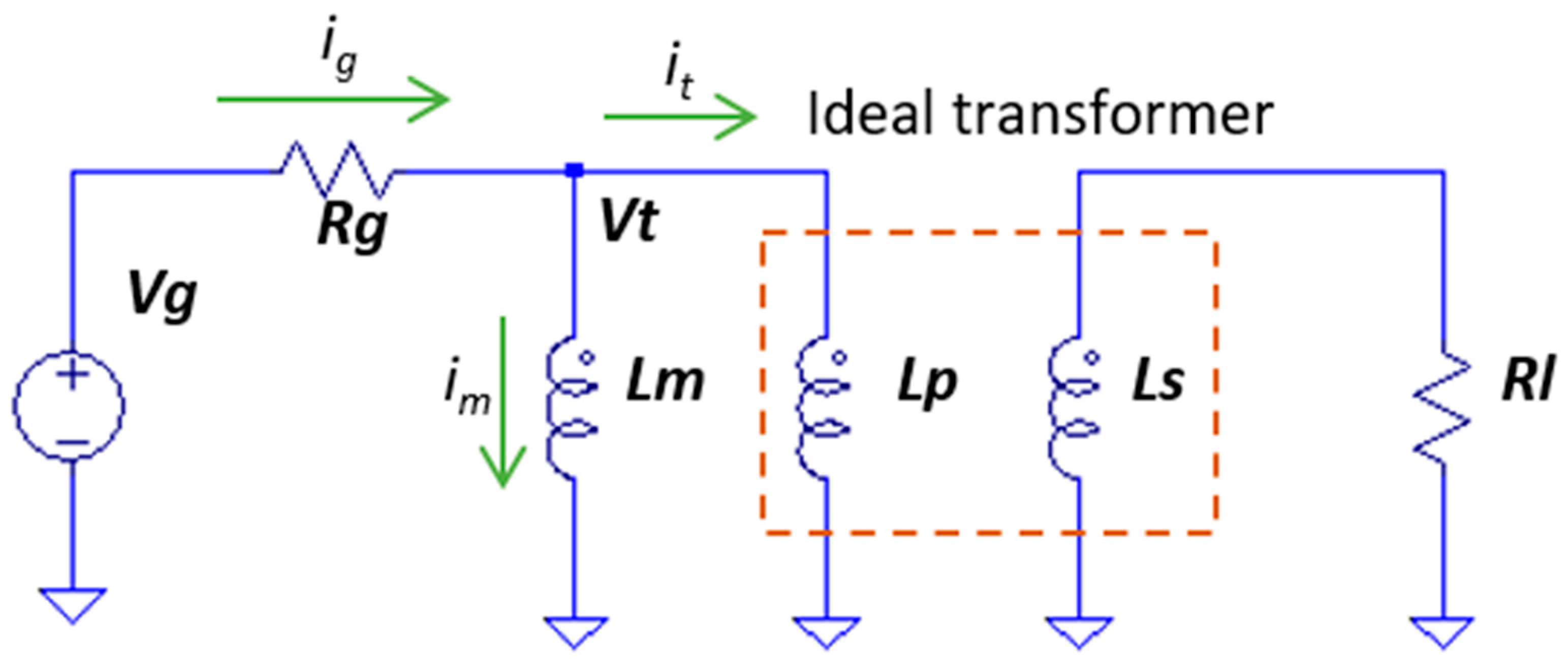
Figure 1 represents the circuital model that will be employed in the following sections. The real transformer is modelled by the magnetization inductance, followed by an ideal transformer, where and are the primary and secondary coils, respectively.
The load resistance, , the generator, and its resistance, complete this simple model. By considering the currents and identified in Figure 1, and by applying the current balance at the electrical node of voltage, , we obtain:
Here, is the load resistance, , moved to the primary side through the transformer ratio, .
By substituting (5)–(7) into (4), it is possible to obtain a differential equation [36] whose analytical solution is the expression of the magnetic flux, [34,35]. The reader interested in the details of the calculations can read Appendix A. The results for the flux and the voltage at the primary coil are reported below:
where:
Apart from the multiplication constant, , the flux features a trend that is the summation of a cosine term that oscillates at frequency, , and an exponential component that decays in time with the temporal constant, . This constant depends on the magnetization inductance and the parallel of the resistors of the generator, , and the load moved to the primary, .
The trend of the flux is important, since it must be contained among the saturation limits. At time = 0, the exponential term predominates; while, for , its contribution is below 5%, and can be safely neglected. In that region, the flux is dominated by the cosine term.
An example can better clarify this point. Let us consider the circuit of Figure 1, where the components have the values reported in Table 1. In this example, we employed a load resistor = 75 Ohm, that corresponds to = 75/4 = 18.75 Ohm through the turn ratio 1:2. The excitation is set to = 20 V, so that the output peaks at 40 V, i.e., 80 Vpp. Figure 2 (top) shows the trend of the magnetic flux, and the voltage, 2, at the load (bottom), both calculated through Equations (8) and (9). As expected, the flux features a cosinusiodal oscillation of amplitude = 2.6 µWb on top of an exponential drift with decay = 10.5 µs. The peak of the flux is near the beginning of the waveform, and its value is = 5.2 µWb. On the other hand, for > 3 = 31.5 µs, the flux is within the ± limits. It is apparent that the most critical condition for the saturation of the transformer core is during the exponential transient, i.e., for < 3.
In other words, while the flux is within the ± limits out of the transient, it reaches during the transient. Thus, a transformer intended for working in the transient region must be selected with a core saturation limit , that is 2-fold with respect to a transformer working out of the transient. Unfortunately, as already noted, this is the case of ultrasound applications, where the excitation is composed of a few sinusoidal cycles transmitted every PRI. In Figure 2, an example of a possible excitation burst, composed by 5 cycles, is highlighted in bold blue. The burst is clearly in the transient region. In conclusion, in ultrasound applications, (3) should rather be modified in:
2.2. The Effects of Core Saturation in Ultrasound Applications
The magnetic flux trend present in the transformer core during the transient (see Figure 2) can easily produce saturation. When the saturation occurs, the magnetization inductance falls down rapidly and a corresponding high current (rush current) is required from the circuits that drives the transformer. In practical conditions, the generator has a limited current capability, which saturates at a given boundary (for example 1–2 A for a high-current operational amplifier). When the required current exceeds the saturation limit of the generator, the driving voltage drops, and wide distortions are produced in the output.
In order to verify and quantify the aforementioned phenomenon, the circuit of Figure 1 was implemented in the circuit simulator LTSpice (Analog Devices, MA, USA). The parameters reported in Table 1 were employed. The core saturation was simulated by imposing a hyperbolic tangent relation between current and flux at the magnetization inductance:
In (12), is the current value where the flux reaches the saturation limit . In this example, we set , corresponding to a saturation threshold of = 2.6 µVs for = 19 µH. A generic operation amplifier, with a current limit of 1A, was used to drive the transformer. The excitation was composed by bursts of 5 sinusoidal cycles. Figure 3 shows, on top, the current flowing in the magnetization inductance, and, on the bottom, the voltage 2 at the load resistor. At the first cycle, the current rapidly rises. As soon as it reaches 1 A, which is the limit of the driver, the voltage drops to 0 V, producing an evident distortion on the output. In the next cycles, the distortion is less evident, but the current is not sinusoidal, which indicates that the transformer core partially saturates. The circuit described in the simulation of Figure 3 was assembled and experimental measurements confirmed the simulations (see Figure 8a,c in the Experimental Section 4.2).
3. The Proposed Solution
3.1. Magnetic Core Prefluxing
The transformer core saturation experienced during the transient can be mitigated by adding a correction current, , flowing in the magnetization inductance [35]. This current should feature a temporal trend suitable to cancel the exponential term present in Equation (8):
where and are defined in (10). With this correction, the magnetization flux becomes:
The flux corrected by injecting the current has a cosinusoidal trend, without the exponential transient that is the source of the difficulties described in the previous paragraphs. The maximum of the flux is now (instead of the 2) and the transformer can be exploited at its maximum saturation capacity.
The correction current, can be generated by pre-charging the magnetization inductance with the current of value:
At the burst start, the pre-charging current, will decay through the magnetization inductance and the equivalent circuit resistance, , with a temporal constant, thus generating the desired current like in (13). The flux Equation (14) is also obtained by mathematically solving the current Equation (4) with the initial condition (15), as detailed in the Appendix B.
In Pulse Wave ultrasound applications, the excitation burst repeats every PRI, thus the correction current should feature the same PRI periodicity. It must be at the beginning of every transmission burst, then it should decay towards 0 with a temporal constant until the burst transmission lasts, and when the burst ends, the current should recover the initial value, to be ready for the beginning of the next burst. The recovery phase, i.e., the trend of the current between the burst end and the start of the next burst, is not particularly critical. However, sudden variation (e.g., current steps) must be avoided since they would induce an unwanted voltage to the transformer output. A suitable recovery trend can be obtained by an exponential with a temporal constant , where is reasonably lower than the PRI (e.g., ). Figure 4 shows the temporal relation between the correction current, (top), and the bursts transmission (bottom). The numerical values are based on the parameters of Table 1. The value at time 0, present at the beginning of the burst, is = −150 mA. During the burst, the current decays with a temporal constant = 10 µs (blue curve). When the burst ends, the value is recovered with a time constant of = 10 µs. In this example, PRI = 50 µs.
3.2. Circuit Implementation
This section discusses how the proposed circuit is realized and integrated in a complete ultrasound transmitter/receiver. Figure 5 shows the front-end of a typical single-channel ultrasound transmitter [23], where the prefluxing circuit, highlighted by a dashed-red border, was added.
Every PRI, the excitation burst is synthetized in the back end, and split in two complementary signals that feed the two power amplifiers, Pa. The amplifiers drive the transformer primary coil in a H-bridge configuration. A capacitor stops the direct current (DC) current generated by possible amplifiers’ offsets from flowing in the coil. The secondary coil is connected to the piezoelectric element of the transducer through the high-voltage switch, Sa. A second switch, Sb, connects the transducer to the receiving section (not shown here) that hosts the Low Noise Amplifier (LNA). During the transmission of the high-voltage excitation, Sa is closed, and Sb is open, to avoid the high voltage from saturating and damaging the LNA. After the excitation is transmitted, the Sb closes and Sa opens, so that the weak received echoes reach the LNA without any noisy interference from the transmission section. Then, the cycle repeats in the next PRIs. If required, a digital control logic in the back end generates the digital commands (Scom) for the switches.
The prefluxing circuit can be added to this architecture, as shown in Figure 5. The voltage reference, Vref, is generated in the back end. This is a static reference, that can be set, for example, by a low-rate performance Digital-to-Analog (DA) converter. Vref is buffered and inverted by Ba. Ba should be capable of sinking the prefluxing current. A maximum value in the order of −300 mA is enough for most of the practical situations. The buffer connects to the transformer secondary coil through the resistor, Ri, and the switch, Sc. The connection to the secondary coil instead of the primary is preferred, since the primary coil has no terminal at the ground voltage reference. The switch, Sc, closes during the receiving part of the PRI, so that the prefluxing current asymptotically reaches the Vref/ value. On the other hand, during the transmission phase, Sc opens, and the current decays according to the temporal constant of the circuit, generating the desired waveform. According to (15), the pre-charging current should be ; however, since it is now deployed in the secondary coil, it should be scaled according to the turn ratio, , of the transformer. At the secondary coil, we apply :
The back end should regulate for obtaining the desired , given by (16):
In (17), we have used the definition of given by (10). For a specific front-end, the , , parameters are known and fixed. However, , and change for different transducers and working conditions. The back-end control electronics should tune according to the current condition by setting the suitable .
4. Experiments and Results
4.1. Experimental Set-Up
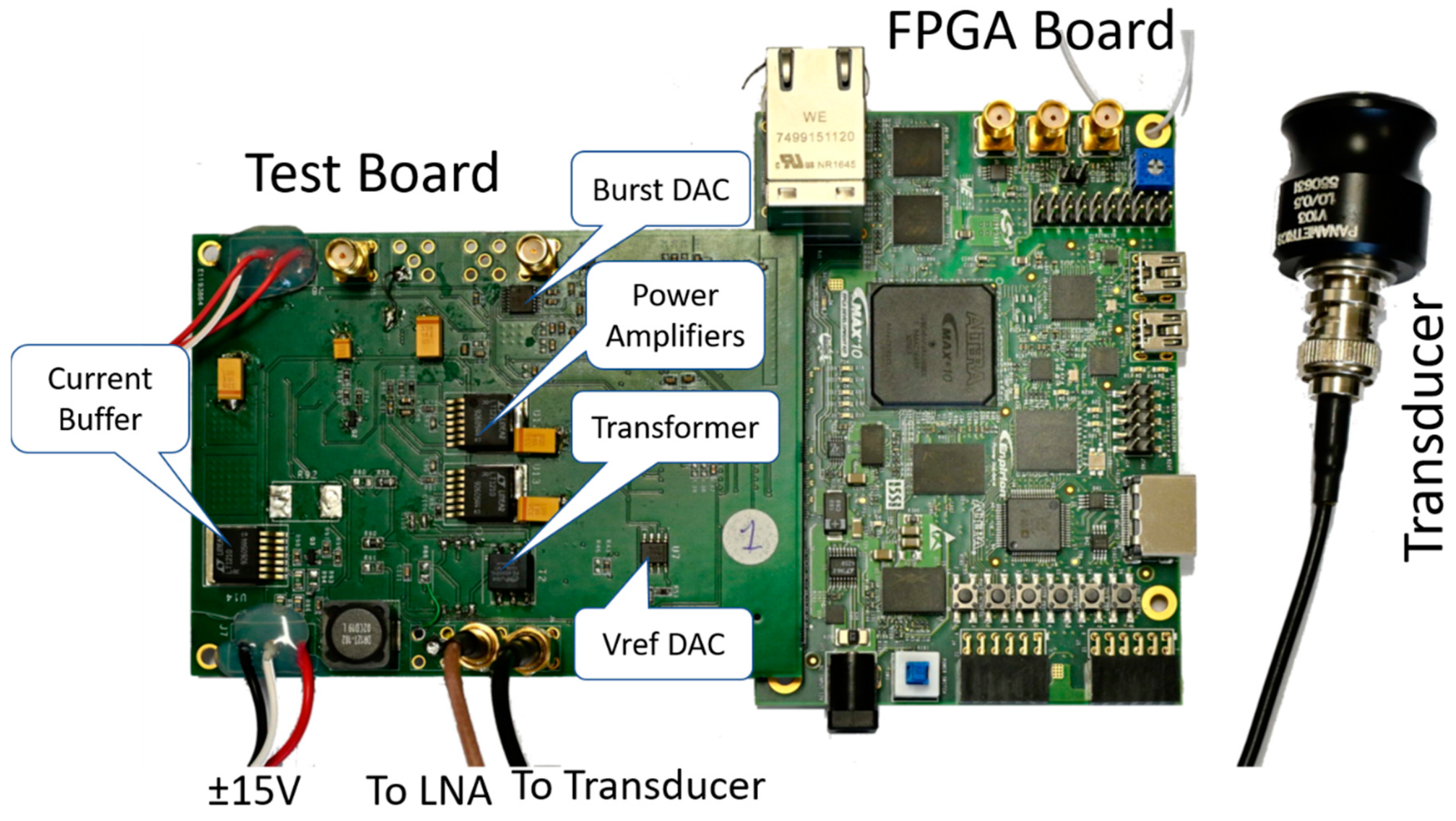
The transmitter circuit of Figure 5 was realized in a house-designed test board. The board includes a high-performance DA converter (AD9707, Analog Devices, MA, USA) for the synthesis of the transmission bursts, followed by an operational amplifier with differential output (ADA4932, Analog Devices, MA, USA) to split the signal. The complementary signals feed two LT1210 (Analog Devices, MA, USA) power amplifiers, which drive the transformer. The LT1210s output up to 1.5 A and are powered at ±15 V. The 2 amplifiers energize the transformer primary coil with up to 40 Vpp, that becomes 80 Vpp at the output of a 1:2 transformer. The output impedance of each amplifier sums, resulting in ≈ 2 Ohm. The high-voltage switches are realized by the MD0100 (Microchip Technology Inc., Arizona, USA) device. This is a particularly easy-to-use switch, since it does not need a digital command, since it is directly controlled by the voltage at its 2 terminals: it opens when the voltage is beyond 2 V and closes otherwise. A simple serial DA converter produces , that is buffered by another LT1210 device connected in inverting configuration. The resistor is 39 Ohm. The board was designed to host commercial transformers with different footprints and features.
The test board was connected to the Intel® MAX® 10 Field Programmagle Gate Array (FPGA) Development Kit (Intel, CA, USA) through the High Speed Mezzanine Card (HMSC) connector. The developing board hosts a Field Programmable Gate Array (FPGA) of the MAX10 family of Intel®. The FPGA was programmed to generate the PRI sequence, and to drive the AD converters in the test board. Figure 6 shows the test board (left) connected to the FPGA board (right). The board drives a 1 MHz Panametrics V103 (Olympus Corp, Japan) transducer. On the bottom of the figure, the output cable toward the receiving board is visible as well.
Two different commercial transformers were employed in the presented experiments: the PE65968NL (Pulse Electronics, CA, USA), with magnetization inductance = 19 uH, and the 78602/2JC (Murata Ps, MA, USA), with magnetization inductance = 380 uH. The maximum magnetic flux is 2.6 and 10 µVs, respectively. The PE65968NL transformer is visible in Figure 6, assembled on the test board. Further parameters that characterize these devices are listed in Table 2. Due to the higher inductance and saturation limit, the 78602/2JC is more suited for a lower frequency range with respect to the PE65968NL.
The ‘1:2CT’ in the turn ratio row in Table 2 indicates that the transformer has the central terminal at the secondary coils, so it can be used with a ratio of 1:1 or 1:2. In this set-up, both transformers were assembled in 1:2 configuration. Please note that the parameters of the implemented circuit, when the PE65968NL transformer is assembled, are the same as those employed in the simulations presented in Section 2 and Section 3 of this paper.
4.2. Experiments
Like already discussed in first part of the paper and confirmed by (3) and (11), the magnetic saturation, for a given excitation, restrains the usable frequency range at its lower margin. Thus, the experiments are focused to investigate if and how the proposed prefluxing circuit helps in overcoming this limitation.
First, with the prefluxing circuit disabled (Sc switch always open), we measured the lower usable frequency for the 2 transformers. The PRI, whose temporal length is not critical, was set to 1 ms. We set = 20 V (80 Vpp at the load) and we connected a scope at the output. Starting from an arbitrary high frequency, we reduced its value until the output showed the waveform distortion typical of core saturation. Saturation occurred at 2.4 MHz and 400 kHz for the PE65968NL and the 78602/2JC, respectively. This result must be compared to the estimates obtained from Equation (11), which calculates the lowest limit at 2.44 MHz and 637 kHz for the PE65968NL and the 78602/2JC, respectively. Both measured values are lower than those calculated by (11), and this is reasonable, since the calculation is based on the data sheet parameters, which represents the worst-case.
In the next step, we computed from (17) the required for activating the prefluxing circuit at a given frequency, obtaining the curves reported in Figure 7 for the 2 transformers. The FPGA was programmed to automatically set the required in the DA converter for the desired frequency burst and the active transformer.
In the final step, we activated the prefluxing circuit, and, starting from the lowest frequency measured in the first step, we further reduced the frequency until saturation again produced a clear distortion in output. Figure 8 shows some screenshots taken from the scope connected to the load. The outputs present with and without the prefluxing circuit are compared. The nominal output, in all the presented cases, is 80 Vpp. The panels in Figure 8a,b refer to the PE65968NL transformer driven with a 3-cycle burst at 1.2 MHz. In Figure 8a, the prefluxing circuit is off, and the positive part of the first cycle presents the clear sign of core saturation, quite similar to the simulation reported in Figure 5. On the other hand, the activation of the prefluxing circuit effectively prevents the saturation. The 78602/2JC transformer, driven by a 2-cycle burst at 200 kHz, shows a similar behavior. Figure 8c shows the output without prefluxing, while in panel d, the output is taken when the circuit is active.
The lowest frequencies usable with prefluxing are 1.2 MHz for PE65968NL and 200 kHz for 78602/2JC. With frequency, the distortion is reduced further due to saturation occurring again. Thus, the prefluxing circuit allows to extend the usable frequencies from 2.4 to 1.2 MHz for PE65968NL, and from 400 to 200 kHz for 78602/2JC. Table 3 summarizes these results. As expected, the lowest frequency limit is improved 2-fold; in fact, given the saturation limit, of the transformer, the lowest frequency with the prefluxing is given by (3) and not by (11).
In the last test, we connected the test board to a Panametrics V103 transducer and an ultrasound board [23], employed here like a receiver. The transducer was driven by 3-cycle bursts at 1.2 MHz through the PE65968NL transformer. The transducer was immersed in degassed water and placed at 2.5 cm from a metallic reflector. Figure 9 shows the received echoes captured from the transducer (Figure 9a) and processed by the ultrasound board through coherent demodulation and envelop detection [37]. The board acquired the main echo around t = 8 µs and the first reverberation around t = 40 µs.
5. Discussion and Conclusions
Small transformers are currently employed in ultrasound transmitters designed to work in the frequency range 100 kHz–10 MHz. Their compact dimension imposes severe constraints on the magnetic core, that can easily saturate at the lowest range of frequencies and/or higher voltages. Moreover, when the transmission is based on short bursts, like in ultrasound applications, the saturation limit is further reduced by a 2-fold factor. In this paper, we proposed a simple circuit that, inspired by the prefluxing technique employed in power network transformers, helps to avoid transformer saturation, thus allowing applications at lower frequency and/or higher voltages. We proposed an implementation and verified the effectiveness of the proposed circuit through experiments and measurements. To the best of our knowledge, this is the first time that the prefluxing technique has been applied to the transformer of an ultrasound transmitter.
The proposed transmitter features a peak power of ≈ 21 W. This value is near the maximum power capability of this class of transmitters. In addition, the use of the transformer restricts the maximum frequency to 10–15 MHz. Applications that would need more power and/or higher frequencies should employ different transmission strategies. This transmitter, in general, features a good energy efficiency, which, however, can be limited by the resistance of the coils. The transformer can represent an important source of radiated noise in the range of the transmitted burst. The problem is reduced by applying shields, but highly sensitive applications can still suffer. The transformer core is susceptible to magnetic interference. The transmitter is not suitable to work in environments where strong magnetic fields are present.
The prefluxing method employed in the network transformers [34,35] is more complex and includes more steps with respect to the implementation presented here. However, the dimensions of the involved transformers and power are extremely different, and justify the proposed simplifications.
The tests were carried out with the two commercial transformers PE65968NL and 78602/2JC, suitable to work in a different frequency range, but the results are more general and can be applied to a wide range of transformers of similar size.
Author Contributions
Conceptualization, methodology, funding acquisition, writing, S.R.; validation, review and editing, D.R. All authors have read and agreed to the published version of the manuscript.
Funding
This research is partially funded by the Ministry of Education, University and Research (MIUR) of the Italian government.
Data Availability Statement
The data presented in this study are available in the article.
Conflicts of Interest
The authors declare no conflict of interest.
Appendix A
In this appendix, the calculation for obtaining the equation that describes the flux in the magnetization inductance of the transformer is detailed. The equations for the current balance at the Vt node of Figure 1 are:
By combining Equations (A1)–(A3), we have the following equation:
By substituting (A4) into (A5), and by considering a sinusoidal excitation of frequency, , , we obtain the following differential equation:
For a simpler notation, we introduce the resistor equal to the parallel of and :
So, Equation (A6) can be rewritten like:
The solution of differential Equation (A8), with the condition = 0, can be obtained through known methods [36], and is:
Equation (A9) represents an exact solution of (A8). However, it can be simplified by applying some reasonable approximations suggested by the typical parameters employed in the ultrasound-specific application. The proposed approximation is:
By applying (A10), we have:
Thus, (A9) becomes:
Finally, the magnetic flux is:
Appendix B
In Appendix A, the flux Equation (A8) is calculated with the initial condition of no current. Here, the flux equation is obtained with the initial condition:
where K is defined in (A10). The solution is:
After applying the approximation reported in (A9)–(A11), we have:
The approximation (A9) can be rewritten as:
Thus, (A17) can be further simplified to:
and the corresponding magnetic flux is:
References
- Cobbold, R.S.C. Foundations of Biomedical Ultrasound; Oxford University Press Inc: Oxford, UK, 2006; ISBN 978-0195168310. [Google Scholar]
- Pandey, G.; Vora, A. Open Electronics for Medical Devices: State-of-Art and Unique Advantages. Electronics 2019, 8, 1256. [Google Scholar] [CrossRef] [Green Version]
- Nakanishi, I.; Maruoka, T. Biometrics Using Electroencephalograms Stimulated by Personal Ultrasound and Multidimensional Nonlinear Features. Electronics 2020, 9, 24. [Google Scholar] [CrossRef] [Green Version]
- Caixinha, M.; Santos, M.; Santos, J. Automatic Cataract Hardness Classification Ex Vivo by Ultrasound Techniques. Ultras Med. Biol. 2016, 42, 989–998. [Google Scholar] [CrossRef]
- Ricci, S.; Ramalli, A.; Bassi, L.; Boni, E.; Tortoli, P. Real-Time Blood Velocity Vector Measurement over a 2-D Region. IEEE Trans. Ultrason. Ferroelect. Freq. Control 2018, 65, 201–209. [Google Scholar] [CrossRef]
- Schmerr, L.W., Jr.; Song, J.-S. Ultrasonic Nondestructive Evaluation Systems; Springer: Berlin/Heidelberg, Germany, 2007; ISBN 978-0-387-49063-2. [Google Scholar]
- Ma, Y.; Shen, H.; Pei, C.; Zhang, H.; Junaid, M.; Wang, Y. Detection of Self-Healing Discharge in Metallized Film Capacitors Using an Ultrasonic Method. Electronics 2020, 9, 1893. [Google Scholar] [CrossRef]
- Lootens, D.; Schumacher, M.; Liard, M.; Jones, S.Z.; Bentz, D.P.; Ricci, S.; Meacci, V. Continuous strength measurements of cement pastes and concretes by the ultrasonic wave reflection method. Constr. Build. Mater. 2020, 242, 117902. [Google Scholar] [CrossRef]
- Marzo, A.; Corkett, T.; Drinkwater, B.W. Ultraino: An Open Phased-Array System for Narrowband Airborne Ultrasound Transmission. IEEE Trans. Ultrason. Ferroelectr. Freq. Control 2018, 65, 102–111. [Google Scholar] [CrossRef] [Green Version]
- Clementi, C.; Littmann, F.; Capineri, L. Identification and Authentication of Copper Canisters for Spent Nuclear Fuel by a Portable Ultrasonic System. IEEE Trans. Ultrason. Ferroelectr. Freq. Control 2020, 67, 1667–1678. [Google Scholar] [CrossRef]
- Dong, X.; Tan, C.; Dong, F. Gas-Liquid Two-Phase Flow Velocity Measurement with Continuous Wave Ultrasonic Doppler and Conductance Sensor. IEEE Trans. Instrum. Meas. 2017, 66, 3064–3076. [Google Scholar] [CrossRef]
- Kotzé, R.; Ricci, S.; Birkhofer, B.; Wiklund, J. Performance tests of a new non-invasive sensor unit and ultrasound electronics. Flow Meas. Instrum. 2015, 48, 104–111. [Google Scholar] [CrossRef]
- Wiklund, J.; Stading, M. Application of in-line ultrasound Doppler-based UVP–PD rheometry method to concentrated model and industrial suspensions. Flow Meas. Instrum. 2008, 19, 171–179. [Google Scholar] [CrossRef]
- Arpaia, P.; Cesaro, U.; Gatti, D.; Moccaldi, N. An Ultrasonic Heading Goniometer Intrinsically Robust to Magnetic Interference. IEEE Trans. Instrum. Meas. 2020, 69, 8735–8743. [Google Scholar] [CrossRef]
- Ricci, S.; Meacci, V. FPGA-Based Doppler Frequency Estimator for Real-Time Velocimetry. Electronics 2020, 9, 456. [Google Scholar] [CrossRef] [Green Version]
- Iula, A.; Micucci, M. Experimental Validation of a Reliable Palmprint Recognition System Based on 2D Ultrasound Images. Electronics 2019, 8, 1393. [Google Scholar] [CrossRef] [Green Version]
- Skjelvareid, M.H.; Birkelund, Y.; Larsen, Y. Internal pipeline inspection using virtual source synthetic aperture ultrasound imaging. NDT E Int. 2013, 54, 151–158. [Google Scholar] [CrossRef]
- Boni, E.; Bassi, L.; Dallai, A.; Guidi, F.; Meacci, V.; Ramalli, A.; Ricci, S.; Tortoli, P. ULA-OP 256: A 256-Channel Open Scanner for Development and Real-Time Implementation of New Ultrasound Methods. IEEE Trans. Ultrason. Ferroelectr. Freq. Control 2016, 63, 1488–1495. [Google Scholar] [CrossRef]
- You, B.Y.S.; Walczak, M.; Lewandowski, M.; Yu, A.C.H. Live Ultrasound Color-Encoded Speckle Imaging Platform for Real-Time Complex Flow Visualization In Vivo. IEEE Trans. Ultrason. Ferroelectr. Freq. Control 2019, 66, 656–668. [Google Scholar] [CrossRef]
- Jensen, J.A.; Holten-Lund, M.F.; Nilsson, R.T.; Hansen, M.; Larsen, U.D.; Domsten, R.P.; Tomov, B.G.; Stuart, M.B.; Nikolov, S.I.; Pihl, M.J.; et al. SARUS: A synthetic aperture real-time ultrasound system. IEEE Trans. Ultrason. Ferroelectr. Freq. Control 2013, 60, 1838–1852. [Google Scholar] [CrossRef] [Green Version]
- Jain, P.; Chen, J.; Murugan, R.; Vajeed, N.; Miriyala, A.; Tang, T. Co-Design of a Highly Integrated, High Peformance, 16-Channel Pulsers and Tx/Rx Switches for Ultrasound Imaging Systems. In Proceedings of the IEEE 70th Electronic Components and Technology Conference (ECTC), Orlando, FL, USA, 3–30 June 2020; pp. 1390–1395. [Google Scholar] [CrossRef]
- Ricci, S.; Bassi, L.; Boni, E.; Dallai, A.; Tortoli, P. Multichannel FPGA-based arbitrary waveform generator for medical ultrasound. Electron. Lett. 2007, 43, 1335–1336. [Google Scholar] [CrossRef]
- Ricci, S.; Meacci, V.; Birkhofer, B.; Wiklund, J. FPGA-based System for In-Line Measurement of Velocity Profiles of Fluids in Industrial Pipe Flow. IEEE Trans. Ind. Electron. 2017, 64, 3997–4005. [Google Scholar] [CrossRef]
- Fiorillo, A.S. Design and characterization of a PVDF ultrasonic range sensor. IEEE Trans. Ultrason. Ferroelectr. Freq. Control 1992, 39, 688–692. [Google Scholar] [CrossRef] [PubMed]
- Savoia, A.S.; Caliano, G.; Pappalardo, M. A CMUT probe for medical ultrasonography: From microfabrication to system integration. IEEE Trans. Ultrason. Ferroelectr. Freq. Control 2012, 59, 1127–1138. [Google Scholar] [CrossRef] [PubMed]
- Joseph, J.; Singh, S.G.; Vanjari, S.R.K. Piezoelectric Micromachined Ultrasonic Transducer Using Silk Piezoelectric Thin Film. IEEE Electron Device Lett. 2018, 39, 749–752. [Google Scholar] [CrossRef]
- Drinkwater, B.W.; Wilcox, P.D. Ultrasonic arrays for non-destructive evaluation: A review. NDT E Int. 2006, 39, 525–541. [Google Scholar] [CrossRef]
- Qiu, W.; Yu, Y.; Tsang, F.K.; Sun, L. A multifunctional, reconfigurable pulse generator for high-frequency ultrasound imaging. IEEE Trans. Ultrason. Ferroelectr. Freq. Control. 2012, 59, 1558–1567. [Google Scholar] [CrossRef]
- Garcia-Rodriguez, M.; Yaez, Y.; Garcia-Hernandez, M.J.; Salazar, J.; Turo, A.; Chavez, J.A. Application of Golay codes to improve the dynamic range in ultrasonic Lamb waves air-coupled systems. NDT E Int. 2010, 43, 677–686. [Google Scholar] [CrossRef]
- Ramalli, A.; Boni, E.; Dallai, A.; Guidi, F.; Ricci, S.; Tortoli, P. Coded Spectral Doppler Imaging: From Simulation to Real-Time Processing. IEEE Trans. Ultrason. Ferroelectr. Freq. Control 2016, 63, 1815–1824. [Google Scholar] [CrossRef] [PubMed]
- Giannelli, P.; Bulletti, A.; Granato, M.; Frattini, G.; Calabrese, G.; Capineri, L. A Five-Level, 1-MHz, Class-D Ultrasonic Driver for Guided-Wave Transducer Arrays. IEEE Trans. Ultrason. Ferroelectr. Freq. Control 2019, 66, 1616–1624. [Google Scholar] [CrossRef]
- Gao, Z.; Gui, P.; Jordanger, R. An Integrated High-Voltage Low-Distortion Current-Feedback Linear Power Amplifier for Ultrasound Transmitters Using Digital Predistortion and Dynamic Current Biasing Techniques. IEEE Trans. Circuits Syst. II Express Briefs 2014, 61, 373–377. [Google Scholar] [CrossRef]
- Svilainis, L. Power amplifier for ultrasonic transducer excitation. Ultragarsas 2006, 1, 30–36. [Google Scholar]
- Ling, P.C.Y.; Basak, A. Investigation of magnetizing inrush current in a single-phase transformer. IEEE Trans. Magn. 1988, 24, 3217–3222. [Google Scholar] [CrossRef]
- Taylor, D.I.; Law, J.D.; Johnson, B.K.; Fischer, N. Single-Phase Transformer Inrush Current Reduction Using Prefluxing. IEEE Trans. Power Deliv. 2012, 27, 245–252. [Google Scholar] [CrossRef]
- Street, R.L. Analysis and Solution of Partial Differential Equations; Brooks/Cole Pub. Co.: Monterey, CA, USA, 1973. [Google Scholar]
- Ricci, S.; Meacci, V. Data-Adaptive Coherent Demodulator for High Dynamics Pulse-Wave Ultrasound Applications. Electronics 2018, 7, 434. [Google Scholar] [CrossRef] [Green Version]
Figure 1.
The real transformer is modelled with the magnetization inductance, followed by an ideal transformer, . The transformer is powered by the generator, , through the resistor, , and it is loaded by .
Figure 1.
The real transformer is modelled with the magnetization inductance, followed by an ideal transformer, . The transformer is powered by the generator, , through the resistor, , and it is loaded by .

Figure 2.
Magnetic flux (top), and voltage at load (bottom) for the described example. The magnetic flux features a transient with exponential decay of time constant, , and maximum near t = 0.
Figure 2.
Magnetic flux (top), and voltage at load (bottom) for the described example. The magnetic flux features a transient with exponential decay of time constant, , and maximum near t = 0.

Figure 3.
Magnetization current (top) and load voltage (bottom) in the circuit of Figure 1 when the transformer features = 2.6 µVs saturation limit and = 19 µH magnetization inductance. During saturation, the driver circuit reaches its 1A current limit, and a voltage distortion appears in output.
Figure 3.
Magnetization current (top) and load voltage (bottom) in the circuit of Figure 1 when the transformer features = 2.6 µVs saturation limit and = 19 µH magnetization inductance. During saturation, the driver circuit reaches its 1A current limit, and a voltage distortion appears in output.

Figure 4.
Correction current (top) and output voltage (bottom) during 2 PRIs of periods of 50 µs each. The current starts from ipre = −150 mA and decays with a 10 µs constant (blue curve) during the burst transmission. At the end of the burst, the current recovers the initial value.
Figure 4.
Correction current (top) and output voltage (bottom) during 2 PRIs of periods of 50 µs each. The current starts from ipre = −150 mA and decays with a 10 µs constant (blue curve) during the burst transmission. At the end of the burst, the current recovers the initial value.

Figure 5.
Architecture of the transmitter circuit with the added prefluxing circuit (dashed-red box). A couple of power amplifiers (Pa) apply complementary signals to the transformer coil. The Sa switch is closed during transmission, while Sc and Sb are closed during reception. During reception, the prefluxing circuit charges the magnetization inductance to -Vref/ current; during transmission, this current decays towards 0.

Figure 6.
The house-designed test board is connected to the commercial FPGA board. In the test board, the power amplifiers, current buffer, burst and Vref DA converter, and the transformer are highlighted. The test board is connected to a Panametrics V103 transducer and to the receiver board (not shown).

Figure 7.
Values of to be employed in input to the prefluxing circuit for the PE65968NL (left) and the 78602/2JC (right) transformers in the frequency range 1–2.5 MHz and 200–400 kHz.
Figure 7.
Values of to be employed in input to the prefluxing circuit for the PE65968NL (left) and the 78602/2JC (right) transformers in the frequency range 1–2.5 MHz and 200–400 kHz.

Figure 8.
Scope screenshots of transmission bursts measured at the load for the 2 tested transformers. The PE65968NL was excited by 3 cycles at 1.2 MHz (a,b), and the 78602/2JC with 2 cycles at 200 kHz (c,d). In (a,c), the prefluxing circuit is not active, while in (b,d), it is active. Output is 80 Vpp in all 4 measurements.

Figure 9.
Echoes acquired from a metallic reflector energized by a 3-cycle burst at 1.2 MHz through the proposed transmitter. (a) Radio frequency echo, and (b) signal after demodulation and envelop detection.
Figure 9.
Echoes acquired from a metallic reflector energized by a 3-cycle burst at 1.2 MHz through the proposed transmitter. (a) Radio frequency echo, and (b) signal after demodulation and envelop detection.


Table 1.
Values of the components for the circuit of Figure 1.
Table 1.
Values of the components for the circuit of Figure 1.
| Parameter | Value |
|---|---|
| 20 V | |
| 2 Ohm | |
| 75 Ohm | |
| 19 µH | |
| (turn ratio) | 1:2 |
| 1.2 MHz | |
| 18.75 Ohm | |
| 1.8 Ohm | |
| 10.5 µs | |
| 2.4 µWb |
Table 2.
Transformers’ features.
| Parameter | PE65968NL | 78602/2JC | |
|---|---|---|---|
| Magnetization inductance | 19 uH | 380 uH | |
| Max Volt-time product | 2.6 µVs | 10 µVs | |
| DC coil resistance | 0.15 Ohm | 0.34 Ohm | |
| Leakage inductance | 0.06 uH | 0.27 uH | |
| Interwinding capacitance | 10 pF | 32 pF | |
| Turns ratio | N | 1:2CT | 1:2CT |
Table 3.
Lowest limit improvement achievable with prefluxing circuit.
| Prefluxing | PE65968NL | 78602/2JC |
|---|---|---|
| off | 2.4 MHz | 400 kHz |
| on | 1.2 MHz | 200 kHz |
Publisher’s Note: MDPI stays neutral with regard to jurisdictional claims in published maps and institutional affiliations. |
© 2021 by the authors. Licensee MDPI, Basel, Switzerland. This article is an open access article distributed under the terms and conditions of the Creative Commons Attribution (CC BY) license (http://creativecommons.org/licenses/by/4.0/).
Share and Cite
MDPI and ACS Style
Ricci, S.; Russo, D. Linear Ultrasound Transmitter Based on Transformer with Improved Saturation Performance. Electronics 2021, 10, 107. https://0-doi-org.brum.beds.ac.uk/10.3390/electronics10020107
AMA Style
Ricci S, Russo D. Linear Ultrasound Transmitter Based on Transformer with Improved Saturation Performance. Electronics. 2021; 10(2):107. https://0-doi-org.brum.beds.ac.uk/10.3390/electronics10020107
Chicago/Turabian StyleRicci, Stefano, and Dario Russo. 2021. "Linear Ultrasound Transmitter Based on Transformer with Improved Saturation Performance" Electronics 10, no. 2: 107. https://0-doi-org.brum.beds.ac.uk/10.3390/electronics10020107
Note that from the first issue of 2016, this journal uses article numbers instead of page numbers. See further details here.