An Effective Decoupling Control with Simple Structure for Induction Motor Drive System Considering Digital Delay

Abstract

Digital processing poses a considerable time delay on controllers of induction motor (IM) driving system, which degrades the effects of torque/flux decoupling, slows the motor torque response down, or even makes the entire system unstable, especially when operating at a low switching frequency. The existing methods, such as feed-forward and feed-back decoupling methods based on the proportional integral controller (PI), have an intrinsic disadvantage in the compromise between high performance and low switching frequency. Besides, the digital delay cannot be well compensated, which may affect the system loop and bring instability. Conventional complex vector decoupling control based on an accurate IM model employs complicated decoupling loops that may be degraded by digital delay leading to discrete error. This article aims to give an alternative complex vector decoupling solution with a simple structure, intended for optimized decoupling and improving the system dynamic performance throughout the entire operating range. The digital delay-caused impacts, including secondary coupling effect and voltage vector amplitude/phase inaccuracy, are specified. Given this, the digital delay impact is canceled accurately in advance, simplifying the entire decoupling process greatly while achieving uncompromised decoupling performance. The simulation and experimental results prove the effectiveness and feasibility of the proposed decoupling technique.

1. Introduction

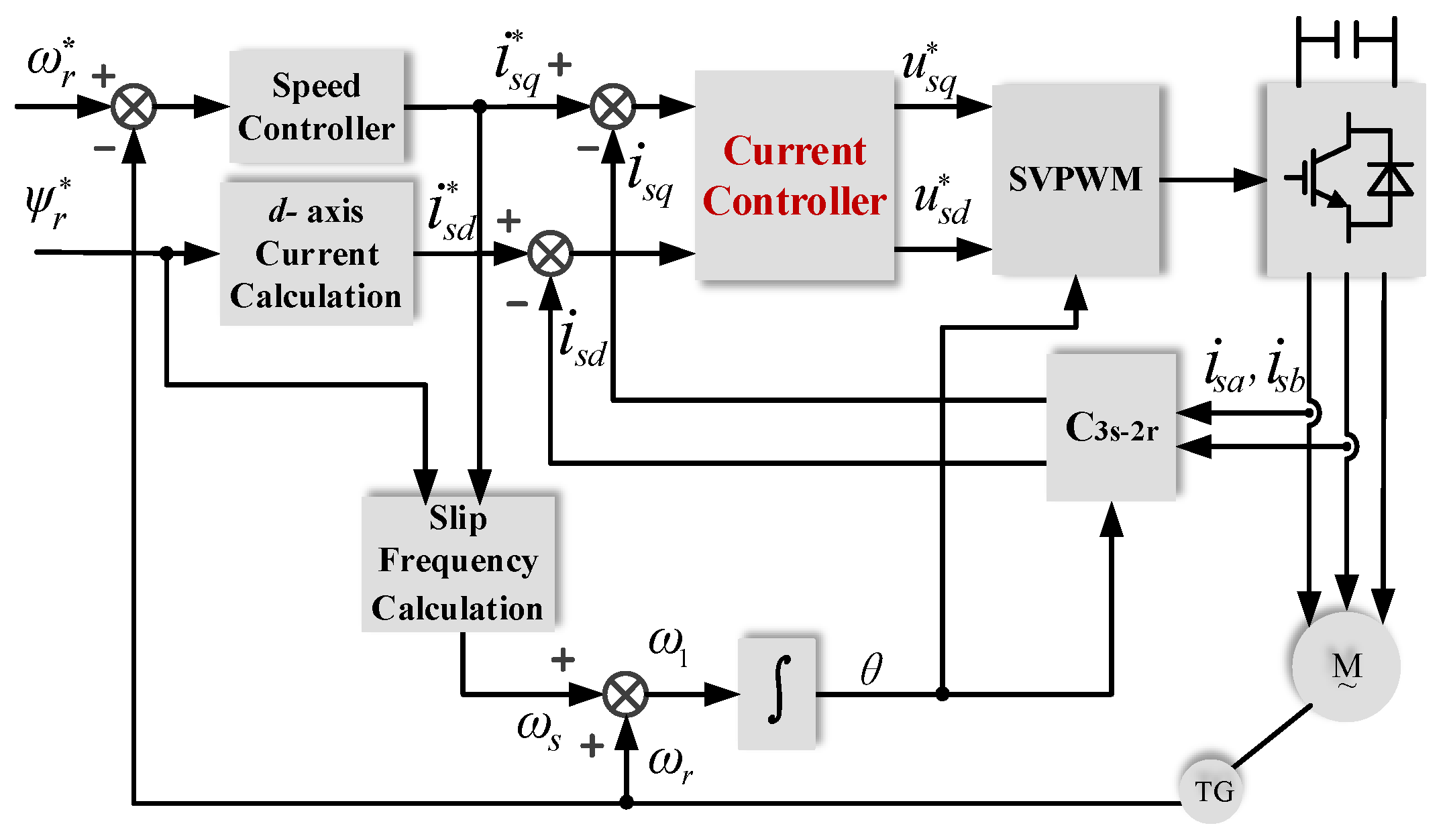
Induction motors (IMs) are widely used in the industry due to their simple structure, fast dynamic response, low moment of inertia, low torque ripple, high reliability, and low costs of manufacture, repair, and maintenance. Particularly because of the multifarious advantages in handling large voltages and currents, the induction motor continues to be a preferred choice for multimegawatt, medium-voltage applications [1,2,3]. To achieve better dynamic performance, more complex and sophisticated techniques were proposed to control the motor [4]. These techniques include Field Oriented Control (FOC) [5], Direct Torque Control (DTC) [6], and Indirect Stator Control (ISC) [7]. Field Oriented Control is the most popular vector control method [8]. Previous studies have shown that due to its high efficiency in controlling the induction motor, this vector control method is by far the most widely used control scheme [9,10]. As shown in Figure 1, FOC is implemented by modulating the torque component and field component of the stator current (i_sq and i_sq) separately, through a synchronized change in supply voltage (u_sq and u_sq) amplitudes, phase, and frequency [11]. FOC decomposes the stator current into mutually perpendicular excitation current and torque current, thus realizing independent regulating of flux and torque. Nevertheless, there is cross-coupling in the FOC, consisting of two parts, i.e., the cross-coupling drawn on the stator side by the rotating coordinate transformation and the coupling of the back electromotive force (EMF) [12].

Cross-coupling degrades current control performance. To solve this problem, control methods including hysteresis control, Proportional Integral (PI) control, and predictive control are modified to include decoupling terms based on the feed-back state [13,14,15,16,17]. However, the decoupling terms always lag actual cross-coupling terms. As a result, these feed-back methods only attenuate rather than eliminate axes cross-coupling. In [18,19,20], a decoupling method based on preprocessing reference current feed-forward was proposed and improved. Feed-forward crossing terms are added onto the PI outputs to compensate for cross-coupling components. Such feed-forward structures rely on coupling voltages estimation and are extremely susceptible to parameter migrations, especially under the situation of low switching frequency [21]. Furthermore, such PI-based decoupling controllers cannot achieve expected high performance with a limited control bandwidth [22]. Evidently, the above decoupling methods are not suitable solutions to high-power IM applications like traction driver systems, where the switching frequency is limited to several hundreds of hertz, typically 500 Hz or lower [23].

Alternatively, low switching frequency produces non-negligible digital delay, aggravating the cross-coupling between the excitation and torque components. Inner current loops are much faster than the outer flux/torque loops, which makes the current loops more sensitive to the digital delay. The digital implementation of inner loop controllers would present an inherent time delay between timing points of current sampling and real gating signal acting. Taking the asymmetrical pulse width modulation (PWM) [24] technique, for example, it feeds the output voltage twice every cycle. The delay will be as large as a one-and-a-half sampling period corresponding to approximately 54 degrees in the electric angle at a condition of 500 Hz switching frequency and 100 Hz synchronous frequency. As such, the stator voltage references given by the controllers are not as expected, which may cause motor instability. In [25], the authors propose a delay compensation approach with a one-step prediction of the stator current. However, its employed latch interface may degrade at very low sampling-to-fundamental frequency ratios. Due to the fact that the complex–coefficient transfer function can easily analyze the cross-coupling of axes, some researchers proposed the complex vector current controller to provide better cross-coupling compensation [26,27,28]. The authors describe a contemporary estimating strategy for IM, adopting relaxed discrete-time approximations. However, the technique is somewhat complicated, and the tested sampling-to-fundamental frequency ratio was not less than 25. Wang et al. proposed an accurate complex vector decoupling control with a closed-loop current observer with a lower sampling-to-fundamental frequency ratio of 8 [29]. However, the models are complicated and challenging for real-time industrial applications.

This paper aims to find an alternative complex vector-based solution for the IM drive system in which the decoupling effect is equal to the complex vector-based accurate solution while avoiding the complicated control implementation structure. This paper proposes an improved complex vector control strategy based on the concept put forward in [29]. By further analyzing the coupling effects considering digital delay, this method can address the coupling issues to a full degree. Since the voltage error caused by digital control delay is canceled, this method can also simplify the synchronous coordinate coefficients model of the vector control system. Thus, the complex vector decoupling control can meanwhile have a simple structure.

Section 2 of this paper analyzes the causes of coupling components at low switching frequency conditions and their influence on motor control. In Section 3, the limitations of conventional decoupling control strategies are discussed. In Section 4, the delay compensation strategy with a simple structure is proposed and followed by the improved complex vector control strategy. To validate the proposed technologies, the simulation and experimental results are presented in Section 5. Section 6 concludes the whole paper.

2. Induction Motor Coupling Issues

2.1. Complex Vector Model and Torque/Flux Coupling Effects

The induction motor is commonly modeled as four sets of equations, i.e., flux equations, voltage equations, torque equations, and motion equations. It is a high-order, nonlinear, and strongly coupled complex system in the three-phase static coordinate system (also known as abc frame). The motor model can be greatly simplified by transforming the abc frame into the synchronous one (also known as dq frame). As such, the voltage equations can be expressed by Equations (1) and (2).

$$\left\{\begin{array}{c}{u}_{sd}=(R_s+\sigma L_{s}s)i_{sd}-\sigma L_s{\omega }_1{i}_{sq}+\frac{L_m}{L_r}s{\psi }_{rd}-\frac{L_m}{L_r}{\omega }_1{\psi }_{rq}\\ u_{sq}=(R_s+\sigma L_{s}s)i_{sq}+\sigma L_s{\omega }_1{i}_{sd}+\frac{L_m}{L_r}s{\psi }_{rq}+\frac{L_m}{L_r}{\omega }_1{\psi }_{rd}\end{array}\right.$$

(1)

$$\left\{\begin{array}{c}0=R_r{i}_{sd}+s{\psi }_{sd}+{\omega }_1{\psi }_{sq}+({\omega }_1-{\omega }_r){\psi }_{rq}\\ 0=R_r{i}_{rd}+s{\psi }_{rd}+{\omega }_1{\psi }_{rq}+({\omega }_1-{\omega }_r){\psi }_{rd}\end{array}\right.$$

(2)

where, $u_{sd}$ and $u_{sq}$ are stator voltages components in dq-Frame, $i_{sd}$ and $i_{sq}$ are dq-stator currents, $i_{rd}$ is d-axis rotor current, ${\psi }_{sd}$ and ${\psi }_{sq}$ are dq-stator fluxes, ${\psi }_{rd}$, ${\psi }_{rq}$ are the dq-rotor linkage fluxes, $R_s$ and $L_s$ are stator resistance and inductance, $R_r$ and $L_r$ are rotor resistance and inductance, $L_m$ is mutual magnetization inductance corresponding to the main flux linkages, $\sigma =1-L_{\mathrm{m}}^2/(L_s{L}_r)$ is flux leakage coefficient, $s$ is differential operator, ${\omega }_1$ is the synchronous angular velocity, and ${\omega }_r$ is the rotor angular velocity.

$$\left\{\begin{array}{c}{\psi }_{sd}=L_s{i}_{sd}+L_m{i}_{rd}\\ {\psi }_{sq}=L_s{i}_{sq}+L_m{i}_{rq}\end{array}\right.$$

(3)

$$\left\{\begin{array}{c}{\psi }_{rd}=L_m{i}_{sd}+L_r{i}_{rd}\\ {\psi }_{rq}=L_m{i}_{sq}+L_r{i}_{rq}\end{array}\right.$$

(4)

$$T_e=\frac{3}{2}{n}_p{L}_m\left(i_{sd}{i}_{rd}-i_{rq}{i}_{sq}\right)$$

(5)

Equations (3) and (4) are the flux equations. The torque equation is expressed by (5), where $n_p$ is motor pole count. The dq-frame and the rotor linkage flux ${\psi }_r$ are relatively static. If d-axis is locked to the direction of rotor linkage flux ${\psi }_r$. It drives ${\psi }_{rd}={\psi }_r$, ${\psi }_{rq}=0$. Then the stator voltage equation can be simplified as:

$$\left\{\begin{array}{c}{u}_{sd}=(R_s+\sigma L_{s}s)i_{sd}-\sigma L_s{\omega }_1{i}_{sq}+\frac{L_m}{L_r}s{\psi }_r\\ u_{sq}=(R_s+\sigma L_{s}s)i_{sq}+\sigma L_s{\omega }_1{i}_{sd}+\frac{L_m}{L_r}{\omega }_1{\psi }_r\end{array}\right.$$

(6)

Further, the complex vector expression can be defined as:

$${\mathit{u}}_{\mathit{s}}=(R_s+\sigma L_{s}s){\mathit{i}}_{\mathit{s}}+j\sigma L_s{\omega }_1{\mathit{i}}_{\mathit{s}}+\frac{L_m}{L_r}s{\mathbf{\psi }}_{\mathit{r}}+j\frac{L_m}{L_r}{\omega }_1{\mathit{\psi }}_{\mathit{r}}$$

(7)

Similarly, the complex vector equation of rotor voltage can be obtained as follows:

$$0=R_r{\mathit{i}}_{\mathit{r}}+s{\mathbf{\psi }}_{\mathit{r}}+j{\omega }_s{\mathbf{\psi }}_{\mathit{r}}$$

(8)

where, ${\mathbf{\omega }}_s={\omega }_1-{\omega }_r$ is the motor slip angle frequency. The complex vector equation of the flux linkage can be written as:

$$\left\{\begin{array}{c}{\mathbf{\psi }}_{\mathit{s}}=L_s{\mathit{i}}_{\mathit{s}}+L_m{\mathit{i}}_{\mathit{r}}\\ {\mathbf{\psi }}_{\mathit{r}}=L_r{\mathit{i}}_{\mathit{r}}+L_m{\mathit{i}}_{\mathit{s}}\end{array}\right.$$

(9)

Since ${\mathit{i}}_{\mathit{r}}$ can be expressed by ${\mathbf{\psi }}_{\mathit{r}}$ and ${\mathit{i}}_{\mathit{s}}$ as

$${\mathit{i}}_{\mathit{r}}=\frac{1}{L_r}{\mathbf{\psi }}_{\mathit{r}}-\frac{L_m}{L_r}{\mathit{i}}_{\mathit{s}}$$

(10)

Equation (8) can be rewritten as:

$${\tau }_{r}s{\mathbf{\psi }}_{\mathit{r}}+{\mathbf{\psi }}_{\mathit{r}}=-j{\omega }_s{\tau }_r{\mathbf{\psi }}_{\mathit{r}}+L_m{\mathit{i}}_{\mathit{s}}$$

(11)

where, ${\tau }_r=L_r/R_r$ is the rotor time constant, Equation (11) is the complex vector equation of the rotor flux linkage in the rotating coordinate system. By substituting Equation (11) for Equation (7), the stator voltage complex vector equation can be further expressed by Equation (12):

$${\mathit{u}}_{\mathit{s}}=(R_s^{\prime }+\sigma L_{s}s){\mathit{i}}_{\mathit{s}}+j\sigma L_s{\omega }_1{\mathit{i}}_{\mathit{s}}-\frac{L_m{R}_r}{L_r^2}(1-j{\omega }_r{\tau }_r){\mathbf{\psi }}_{\mathit{r}}$$

(12)

where, $R_s^{\prime }=R_s+{(L_m/L_r)}^2{R}_r$ is the equivalent stator resistance. By substituting Equation (11) into Equation (12), a transfer function can be obtained as:

$$G_m=\frac{{\mathit{i}}_{\mathit{s}}}{{\mathit{u}}_{\mathit{s}}}=\frac{{\tau }_{r}s+j{\omega }_s{\tau }_r+1}{(R_s^{\prime }+\sigma L_{s}s+j\sigma L_s{\omega }_1)({\tau }_{r}s+j{\omega }_s{\tau }_r+1)-k_1(1-j{\omega }_r{\tau }_r)}$$

(13)

where, $k_1=L_m^2{R}_r/L_r^2$, ${\omega }_1$ is the synchronous angular frequency, ${\omega }_r$ is the rotor angular frequency, and ${\omega }_s$ is the slip angular frequency. According to (13), the motor voltage equation in the synchronous rotation coordinate system contains the cross-coupling component $-j\sigma L_s{\omega }_1{\mathit{i}}_{\mathit{s}}$ and the back-EMF component $L_m{R}_r(1-j{\omega }_r{\tau }_r){\psi }_r/L_r^2$. The signal flow diagram of the induction motor in the dq-frame can be illustrated by Figure 2. Coupling parts are caused by the complex factor j. The imaginary part of a complex transfer function determines the degree of current cross-coupling [25]. As shown, there is a coupling factor in the feed-back loop at the rotor side. Generally, the value of the slip angle frequency in the whole speed range is tiny. The value of the rotor time constant is also small. Therefore, the influence of this part of coupling on the motor’s dynamic performance can be ignored.

The second coupling factor in the feed-back loop is at the stator side. The coupling value increases with the increase in the synchronous angular frequency. That is why the current coupling in the middle and high-speed section of the motor is aggravated. Lastly, there is a coupling component between the stator and rotor of the motor. Its degree depends on the size of $j{\omega }_r{\tau }_r{\mathbf{\psi }}_{\mathit{r}}{L}_m{R}_r/L_r^2$, which is proportional to the angular frequency of the rotor. Therefore, the coupling of this part is also aggravated in the middle and high-speed sections.

2.2. Impact of Digital Delay on Coupling Effects

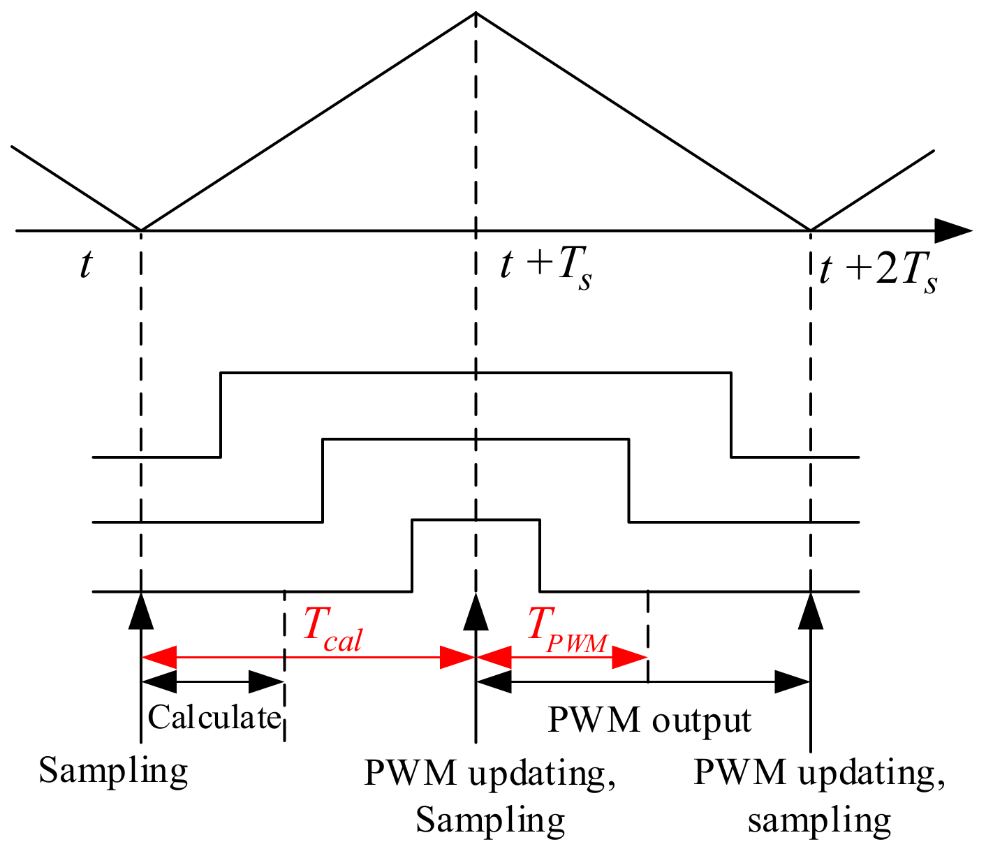
The delay of digital control is another critical factor that can introduce cross-coupling components between the d and q axis voltages. Figure 3 shows the digital control timing of the current control loop, where Space Vector Pulse Width Modulation (SVPWM) is adapted.

Modulated vector voltages contain harmonics. However, the values of the harmonic are crossing zero at midpoints of zero-vectors action time. Hence, the fundamental current component can be obtained by sampling at the middle timing of each zero-vector action interval [30]. At the same time, updating the modulation reference signal at the peak or trough of the carrier wave can help avoid multiple actions within a cycle and false pulses. Therefore, signal sampling and processing are usually carried out in the trough and peak of the carrier wave.

The code execution of control algorithms needs to be completed in advance of the updating of modulated wave data. In other words, the signal processing should be completed before entering the next time step. If we define the current sampling period as $T_s$ then the delay time caused by digital control ($T_{cal}$) equals $T_s$.

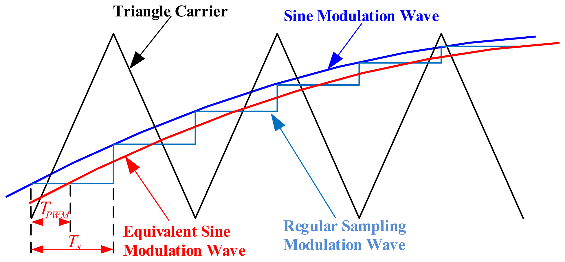
Additionally, the phase delay caused by regular asymmetric sampling is shown in Figure 4. The PWM signal to update is generated during the time interval between two sampling points. An equivalent sine wave can be used to analyze the delay impact caused by PWM modulation. The equivalent sine modulation wave phase is about half a sampling cycle behind the standard sine modulation wave. Therefore, the PWM phase delay caused by the asymmetric regular sampling modulation process is half a sampling period $T_{PWM}=0.5T_s$. Therefore, the total delay time of the digital control system is ${\tau }_d=T_{cal}+T_{PWM}=1.5T_s$.

The delay of the PWM waveform is directly reflected in the tracking delay of the voltage imposed on the IM stators. Such a delay link can be represented by a transfer function approximately equivalent to a first-order inertia link, as expressed by (14).

$$G_{delay}=\frac{{\mathit{u}}_{\mathit{s}}}{{\mathit{u}}_{\mathit{s}}^{\ast }}=\frac{1}{1+{\tau }_{d}s}$$

(14)

Equation (14) can be further expanded into a dynamic equation in the stationary coordinate system as:

$${\tau }_d\frac{d{\mathit{u}}_{\mathit{s}}^{\mathit{s}}}{dt}+{\mathit{u}}_{\mathit{s}}^{\mathit{s}}={\mathit{u}}_{\mathit{s}}^{\mathit{s}\ast }$$

(15)

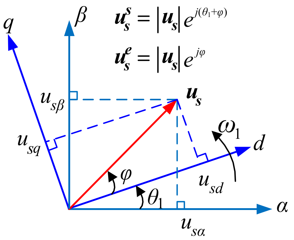
As shown in Figure 5, the voltage complex vector in the stationary coordinate system can be expressed by a corresponding vector in the rotating coordinate system:

$$\left\{\begin{array}{c}{\mathit{u}}_{\mathit{s}}^{\mathit{s}}={\mathit{u}}_{\mathit{s}}^{\mathit{e}}{e}^{j{\omega }_{1}t}\\ {\mathit{u}}_{\mathit{s}}^{\mathit{s}\ast }={\mathit{u}}_{\mathit{s}}^{\mathit{e}\ast }{e}^{j{\omega }_{1}t}\end{array}\right.$$

(16)

Substituting (16) into (15), the voltage equation in the synchronous rotating coordinate system can be obtained as:

$${\tau }_d\frac{d{\mathit{u}}_{\mathit{s}}^{\mathit{e}}}{dt}+(1+j{\omega }_1{\tau }_d){\mathit{u}}_{\mathit{s}}^{\mathit{e}}={\mathit{u}}_{\mathit{s}}^{\mathit{e}\ast }$$

(17)

Therefore, the transfer function of the digital control delay link in the synchronous rotating coordinate system can be obtained as:

$$G_{delay}^e=\frac{{\mathit{u}}_{\mathit{s}}^{\mathit{e}}}{{\mathit{u}}_{\mathit{s}}^{\mathit{e}\ast }}=\frac{1}{1+{\tau }_{d}s+j{\omega }_1{\tau }_d}$$

(18)

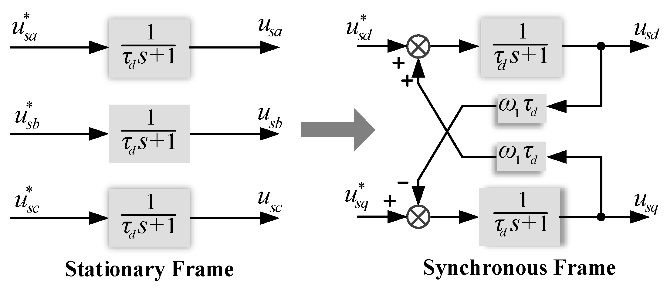
Substituting ${\mathit{u}}_{\mathit{s}}^{\mathit{e}}=u_{sd}+j{u}_{sq}$, ${\mathit{u}}_{\mathit{s}}^{\mathit{e}\ast }=u_{sd}^{\ast }+j{u}_{sq}^{\ast }$ into Equation (18), we can get:

$$\left\{\begin{array}{c}{u}_{sd}=\frac{u_{sd}^{\ast }+{\omega }_1{\tau }_d{u}_{sq}}{{\tau }_{d}s+1}\\ u_{sq}=\frac{u_{sq}^{\ast }-{\omega }_1{\tau }_d{u}_{sd}}{{\tau }_{d}s+1}\end{array}\right.$$

(19)

Figure 6 shows the coupling effect of digital control delay in the rotating coordinate system. Evidently, with the increase in the synchronous angular velocity, the voltage coupling of the d and q axes increases. Although this coupling effect is straightforward as analyzed, it is rarely mentioned in early research. In this paper, such a digital delay leading to cross-coupling is put forward as one critical issue to handle.

3. Conventional Current Decoupling Control Strategies

3.1. PI Current Controller-Based Decoupling

Equation (20) represents the transfer function between the stator current and the stator voltage, derived from (7). It should be noted that the dynamics interval of the rotor flux is often considered to be much shorter than that of the motor current. Hence, the coupling components of the back electromotive force are often designated as external disturbances. Therefore, (20) presents a simplified IM vector model in the synchronous coordinate system.

$$G_p=\frac{{\mathit{i}}_{\mathit{s}}}{{\mathit{u}}_{\mathit{s}}}=\frac{1}{R_s^{\prime }+\sigma L_{s}s+j\sigma L_s{\omega }_1}$$

(20)

To decouple the torque and flux control, two representatives of the PI current regulator with compensation were commonly used. One is to construct compensation terms using the current reference value directly, which is called a feed-forward manner. The other is to construct voltage decoupling terms using sampled real current value, known as feed-back decoupling control.

3.1.1. Feed-Forward Decoupling Control

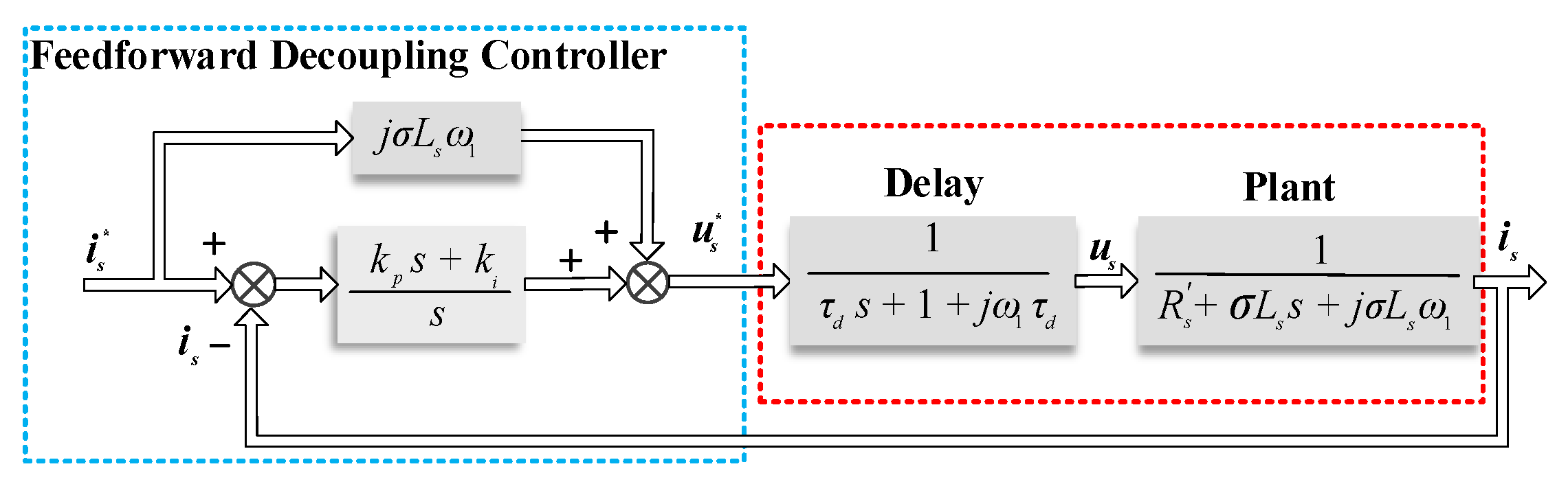
The block diagram of feed-forward decoupling control is shown in Figure 7. The term $j\sigma L_s{\omega }_1{\mathit{i}}_{\mathit{s}}^{*}$ is added to the output of the current controller to compensate for the cross-coupling term. The closed-loop transfer function with PI feed-forward control is:

$$G_{clo}=\frac{k_{p}s+k_i}{s(1+{\tau }_{d}s+j{\omega }_1{\tau }_d)(R_s^{\prime }+\sigma L_{s}s+j\sigma L_s{\omega }_1)+k_{p}s+k_i}$$

(21)

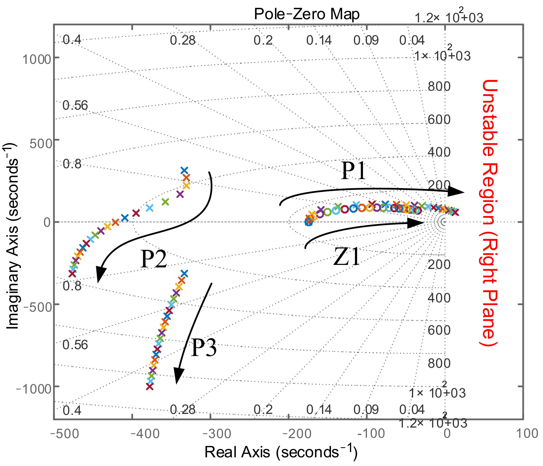
Figure 8 illustrates the zero-pole map of the system. It has one zero and three poles. When the speed is zero, the system is not coupled (P2 and P3 are symmetrical about the real axis). With the synchronization frequency increasing, the poles P2 and P3 are no longer symmetrical to each other about the real axis. Both the pole P1 and the zero Z1 move towards the imaginary axis with the increasing synchronous frequency. Furthermore, Z1 cannot fully offset P1. When the synchronous frequency is high enough, P1 appears at the right unstable region. The system stability is disturbed. Therefore, the feed-forward decoupling has its limitation.

3.1.2. Feed-Back Decoupling Control

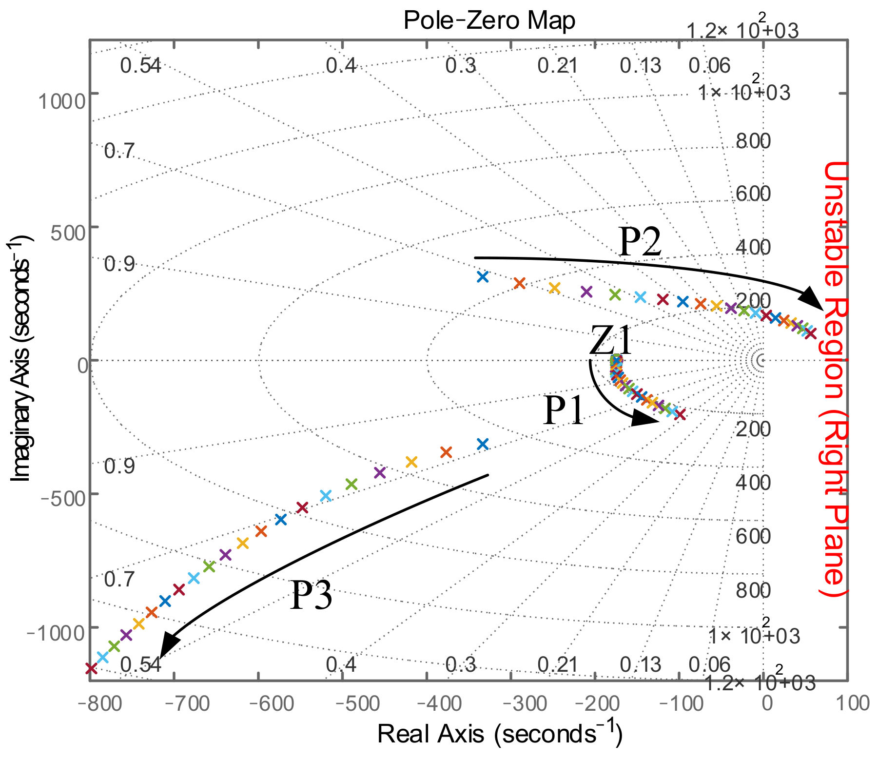
The control block of feed-back decoupling control is shown in Figure 9. The closed-loop transfer function can be derived as:

$$G_{clo}=\frac{k_{p}s+k_i}{s({\tau }_{d}s+1+j{\omega }_1{\tau }_d)(R_s^{\prime }+\sigma L_{s}s+j\sigma L_s{\omega }_1)+k_{p}s+k_i-j{\omega }_1\sigma L_{s}s}$$

(22)

The zero-pole distribution of the feed-back decoupling is illustrated in Figure 10. With the increase in the synchronization frequency, both poles of P1 and P2 move to the imaginary axis. The pole P2 even moves towards the right half-plane with higher speed. Thus, the decoupling effect of feed-back decoupling control is also limited. The goal of conventional decoupling methods is to compensate for the cross-coupling caused by the rotation coordinate transformation. The digital delay leading coupling and the back-EMF coupling is not considered. Hence, it is not hard to know why their decoupling effects are not ideal.

3.2. Complex Vector Current Controller-Based Accurate Motor Model

The two current controllers analyzed above are based on the simplified motor model (see Equation (20)), where the back-EMF coupling component is considered an external disturbance. However, with the increase in the motor speed, the EMF component gradually increases. As such, this coupling part should not be ignored. The accurate mathematical model of the induction motor, which considers all the coupling factors, can be employed to design a current controller contributing more thoroughly to the decoupling effect. When the delay link is taken further into account, the complex vector transfer function becomes:

$$G_p=\frac{{\mathit{i}}_{\mathit{s}}}{{\mathit{u}}_{\mathit{s}}^{\ast }}=\frac{1}{{\tau }_{d}s+1+j{\omega }_1{\tau }_d}\times \frac{{\tau }_{r}s+j{\omega }_s{\tau }_r+1}{(R_s^{\prime }+\sigma L_{s}s+j\sigma L_s{\omega }_1)({\tau }_{r}s+j{\omega }_s{\tau }_r+1)-k_1(1-j{\omega }_r{\tau }_r)}$$

(23)

According to the pole-zero cancellation principle, the complex vector current controller can be designed as:

$$G_c=k_0\frac{{\tau }_{d}s+1+j{\omega }_1{\tau }_d}{{\tau }_{d}s+1}\times \frac{(R_s^{\prime }+\sigma L_{s}s+j\sigma L_s{\omega }_1)({\tau }_{r}s+j{\omega }_s{\tau }_r+1)-k_1(1-j{\omega }_r{\tau }_r)}{{\tau }_{i}s({\tau }_{r}s+j{\omega }_s{\tau }_r+1)}$$

(24)

In this way, the complex vector transfer function is changed into a real one. The coupling of the system caused by the complex poles is therefore compensated. In (24), if the molecule has higher order than the denominator, the controller is equivalent to a differentiator that is easily interfered with by noise and may disturb the stable operation.

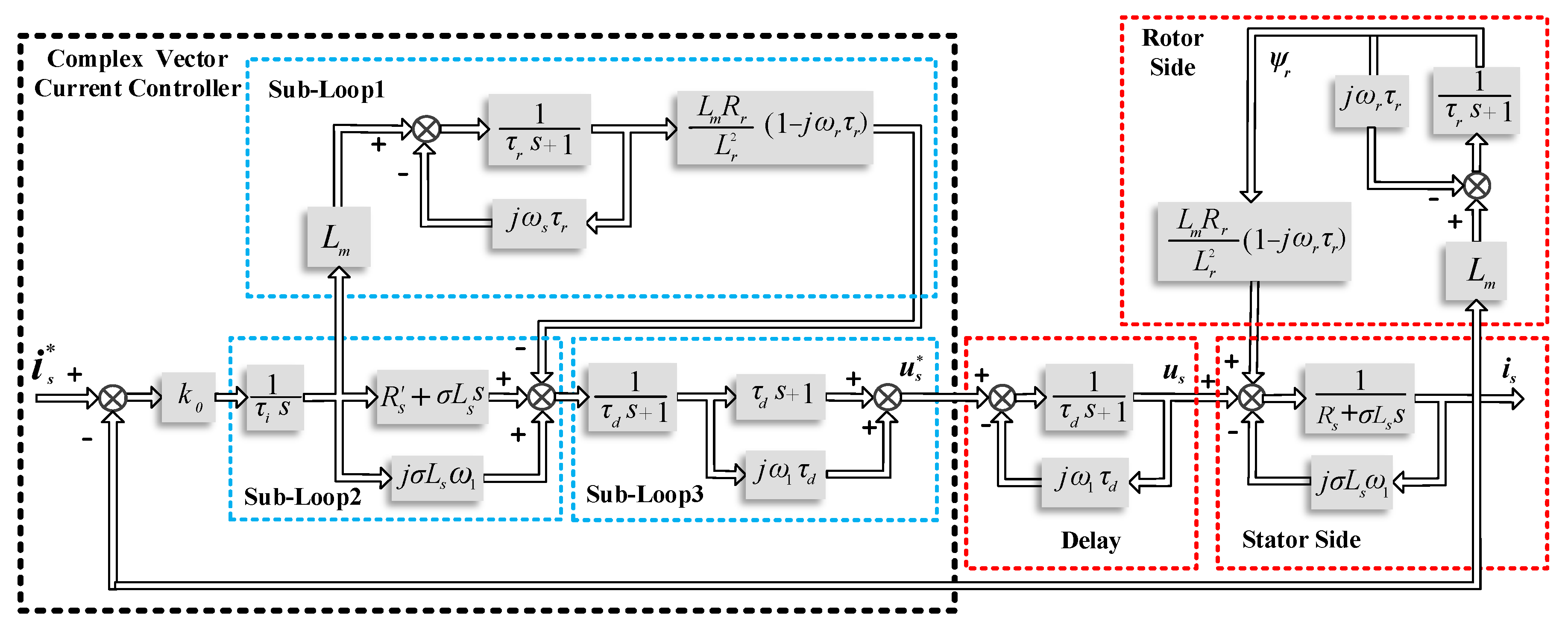
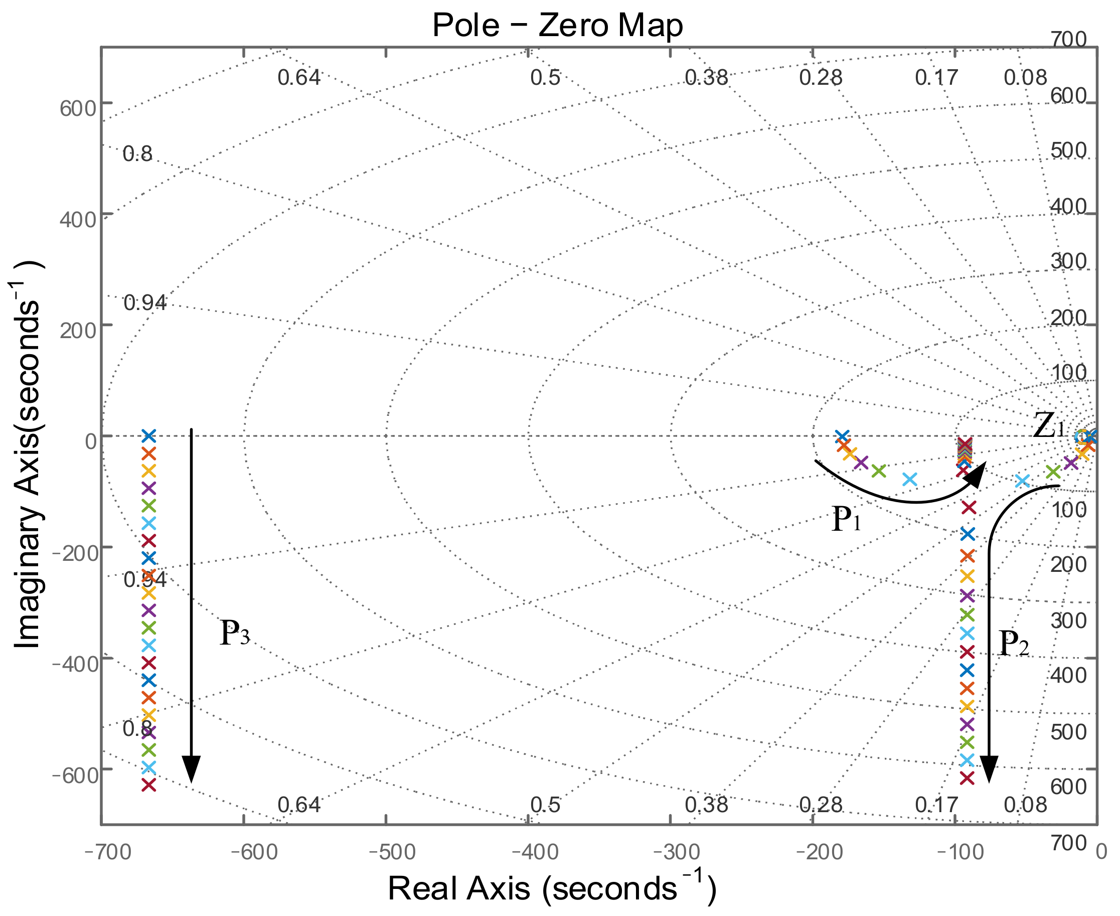
Therefore, a first-order lag link $1/({\tau }_{d}s+1)$ and integral link $1/{\tau }_{i}s$ are introduced. The block diagram for the complex vector current controller of (24) is shown in Figure 11. Three sub-loops contribute to decoupling. Specifically, Sub-loop 1 is used to cancel the complex poles generated by the inverse electromotive force, Sub-loop 2 is used to cancel the complex poles generated by the abc-dq transformation of the motor model, and Sub-loop 3 is used to cancel the complex poles caused by the digital delay. Figure 12 shows the zero-pole distribution of the precise motor model.

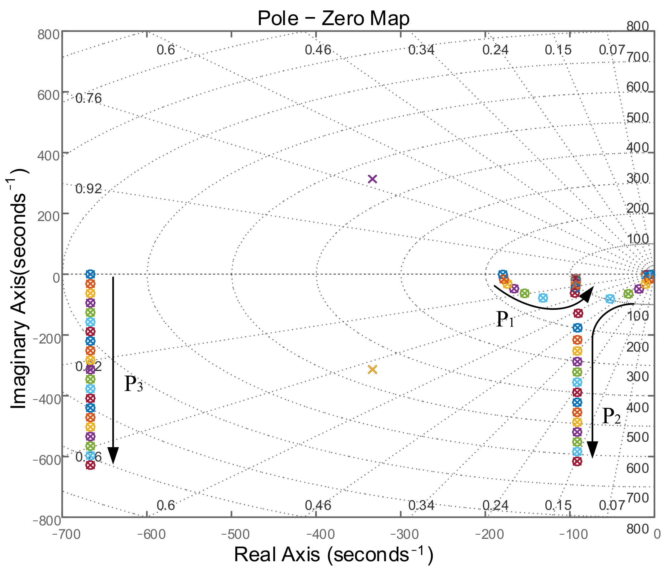
After employing the complex vector current control of (24), the zero-pole distribution of the closed-loop transfer function of the system is shown in Figure 13. By comparing Figure 12 and Figure 13, it can be seen that, except for two conjugate poles, all the other complex poles are offset by the zeros introduced by the complex vector current controller. The complete decoupling is hence realized. The open-loop transfer function of the system can be expressed as:

$$G_0=G_c·G_P=k_0\frac{1}{{\tau }_{i}s({\tau }_{d}s+1)}$$

(25)

As such, the system turns to be a simple second-order one. The imaginary part of transfer function becomes zero. The value of ${\tau }_i$ and $k_0$ can be easily decided according to the desired output characteristics.

Theoretically, the complex vector controller based on an accurate IM model has an excellent decoupling effect. However, the discretization process can be highly complicated. Furthermore, this method is greatly affected by the accuracy of the discretization method, which is often not high at low switching frequencies. Hence, the effort in this paper is to find an alternative complex vector-based solution for the IM drive system so that the decoupling effect is equal to the complex vector-based accurate solution while the complicated control implementation structure can be avoided.

4. Proposed Improved Complex Vector Current Decoupling Control

4.1. Digital Control Delay Compensation

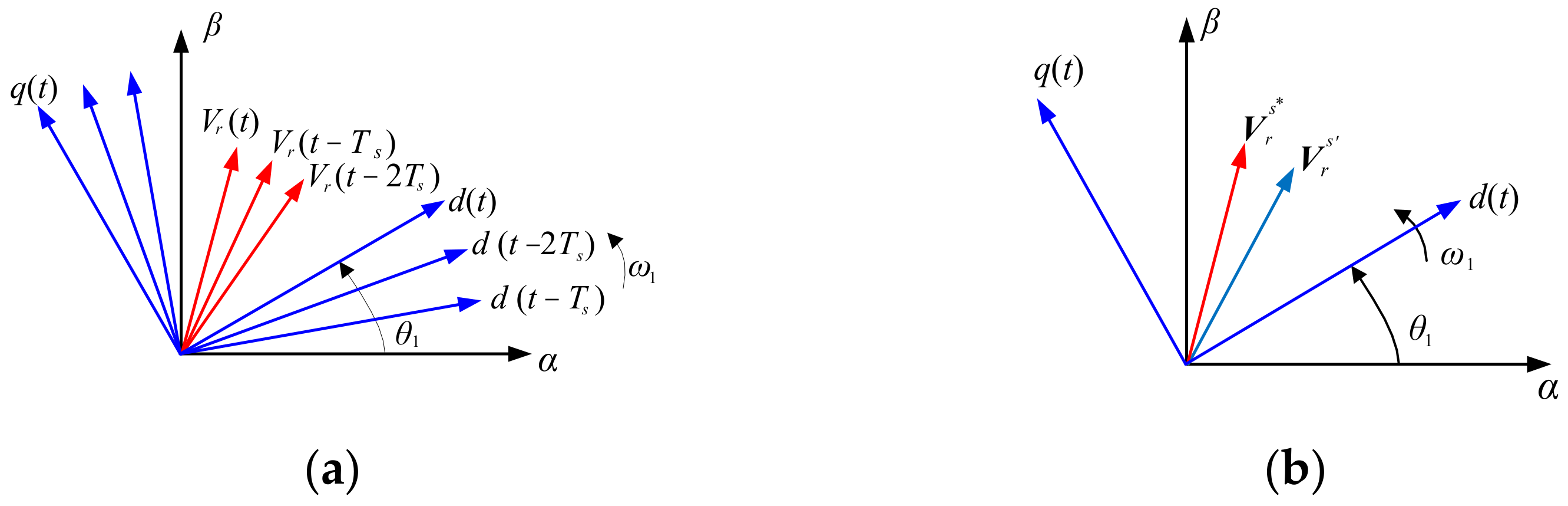
Regarding the space vector pulsed width modulation (SVPWM), due to the presence of digital delay, the voltage space vector (taking a common vector V_r for example) sampled at time t would not act on the power hardware until it enters the time interval between t + T_s and t + 2T_s. Such an effect can also be stated as follow: when the reference space vector ${\mathit{V}}_{\mathit{r}}^{\mathit{s}\ast }$ is aligned with V_r(t), the acting space vector ${\mathit{V}}_{\mathit{r}}^{{\mathit{s}}^{\prime }}$ is actually located inside the sector between V_r (t − T_s) and V_r (t − 2T_s), as shown in Figure 14a. Note that the superscript (${}^s$) is used to indicate the variable is in the static frame (αβ). Another superscript (${}^e$) will be used to indicate the variable is the synchronous frame (dq) in the following analysis.

The rotation speed of the voltage vector ${\mathit{V}}_{\mathit{r}}^{\mathit{s}\ast }$ is consistent with that of the synchronous coordinate frame, so the transformed voltage vector in the synchronous coordinate frame ${\mathit{V}}_{\mathit{r}}^{\mathit{e}\ast }$ (${\mathit{V}}_{\mathit{r}}^{\mathit{e}\ast }={\mathit{V}}_{\mathit{r}}^{\mathit{s}\ast }{e}^{-j{\theta }_1}$) is constant and relatively static with the d-axis. Assuming that the synchronous angular frequency ${\omega }_1$ is invariant during the delay period, from the view of static coordinate system, when the voltage vector ${\mathit{V}}_{\mathit{r}}$ is at the ${\mathit{V}}_{\mathit{r}}^{\mathit{s}\ast }$ position, the real acting vector is ${\mathit{V}}_{\mathit{r}}^{{\mathit{s}}^{\prime }}$, as shown in Figure 14b. Based on area equalization concept [31], the real voltage vector acting on the motor can be expressed by (26):

$${\mathit{V}}_{\mathit{r}}^{{\mathit{s}}^{\prime }}=\frac{1}{T_s}{\displaystyle {\int }_{-2T_s}^{-T_s}{\mathit{V}}_{\mathit{r}}^{\mathit{e}\ast }{e}^{j({\omega }_{1}t+{\theta }_1)}d\tau }=K({\omega }_1,T_s)e^{j({\theta }_1-1.5{\omega }_1{T}_s)}{\mathit{V}}_{\mathit{r}}^{\mathit{e}\ast }$$

(26)

Then it can be derived that the error caused by the digital delay on the voltage vector V_r is:

$$G_{error}=\frac{{\mathit{V}}_{\mathit{r}}^{s^{\prime }}}{{\mathit{V}}_{\mathit{r}}^{\mathit{s}\ast }}=\frac{K({\omega }_1,T_s)e^{j({\theta }_1-1.5{\omega }_1{T}_s)}{\mathit{V}}_{\mathit{r}}^{\mathit{e}\ast }}{{\mathit{V}}_{\mathit{r}}^{\mathit{e}\ast }{e}^{j{\theta }_1}}=K({\omega }_1,T_s)e^{-j1.5{\omega }_1{T}_s}$$

(27)

where, $K({\omega }_1,T_s)=\frac{2}{{\omega }_1{T}_s}\sin (\frac{{\omega }_1{T}_s}{2})$. According to (27), the influence of digital control delay on the voltage space vector can be summarized as follows:

(1)

The voltage vector amplitude becomes $K({\omega }_1,T_s)$ times the reference value. Due to the fact of $K({\omega }_1,T_s)<1$, the amplitude of the voltage vector turns smaller. However, if ${\omega }_1$ is small enough, $K({\omega }_1,T_s)$ would be very close to 1. Hence, the voltage amplitude changes very lightly in the low-speed region.

(2)

The phase lag of the voltage vector occurs, and the lag time is one and a half of sampling cycles. With the increase in the synchronous frequency, the lag angle becomes larger.

By inverting the error formula, a compensation method of the digital delay can be designed as follows:

$$G_c=\frac{1}{G_{error}}=\frac{e^{j1.5{\omega }_1{T}_s}}{K({\omega }_1,T_s)}$$

(28)

Such a method is very straightforward. By employing it to the voltage vector’s amplitude in the stationary coordinate system and the phase correction angle, the magnitude of the voltage vector becomes the same as the original value.

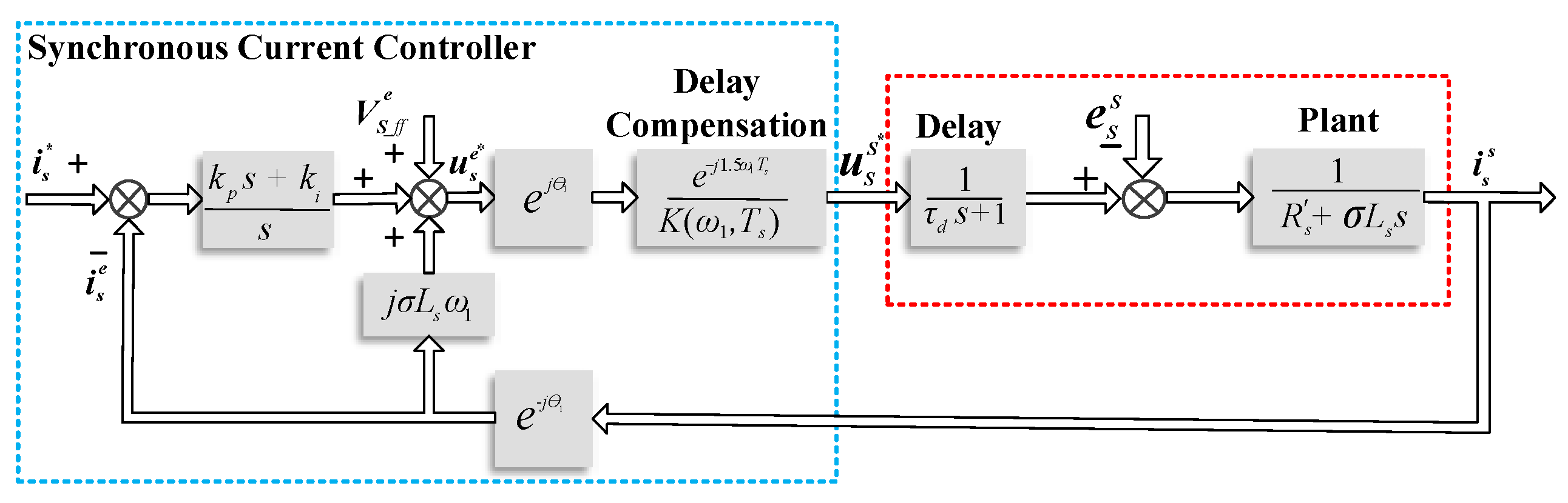
According to the above analysis, the digital delay can be approximately regarded as a first-order inertia link in the static coordinate system. Figure 15 shows the induction motor’s PI-based control block diagram after the delay compensation link (see (28)). In the loop, the term ${\mathit{V}}_{\mathit{s}\_\mathit{f}\mathit{f}}^{\mathit{e}}$ is used to compensate for the back EMF coupling.

$${\mathit{V}}_{\mathit{s}\_\mathit{f}\mathit{f}}^{\mathit{e}}={\mathit{e}}_{\mathit{s}}^{\mathit{e}}={\mathit{e}}_{\mathit{s}}^{\mathit{s}}=-\frac{L_m}{L_r}{\omega }_{br}{\mathbf{\psi }}_{\mathit{r}}$$

(29)

where, ${\omega }_{br}=R_r/L_r-j{\omega }_r$, ${\mathit{e}}_{\mathit{s}}^{\mathit{s}}$ is the back-EMF component in the stationary coordinate system, and ${\mathit{e}}_{\mathit{s}}^{\mathit{e}}$ is the back-EMF component in the synchronous coordinate system. These two are actually same with each other.

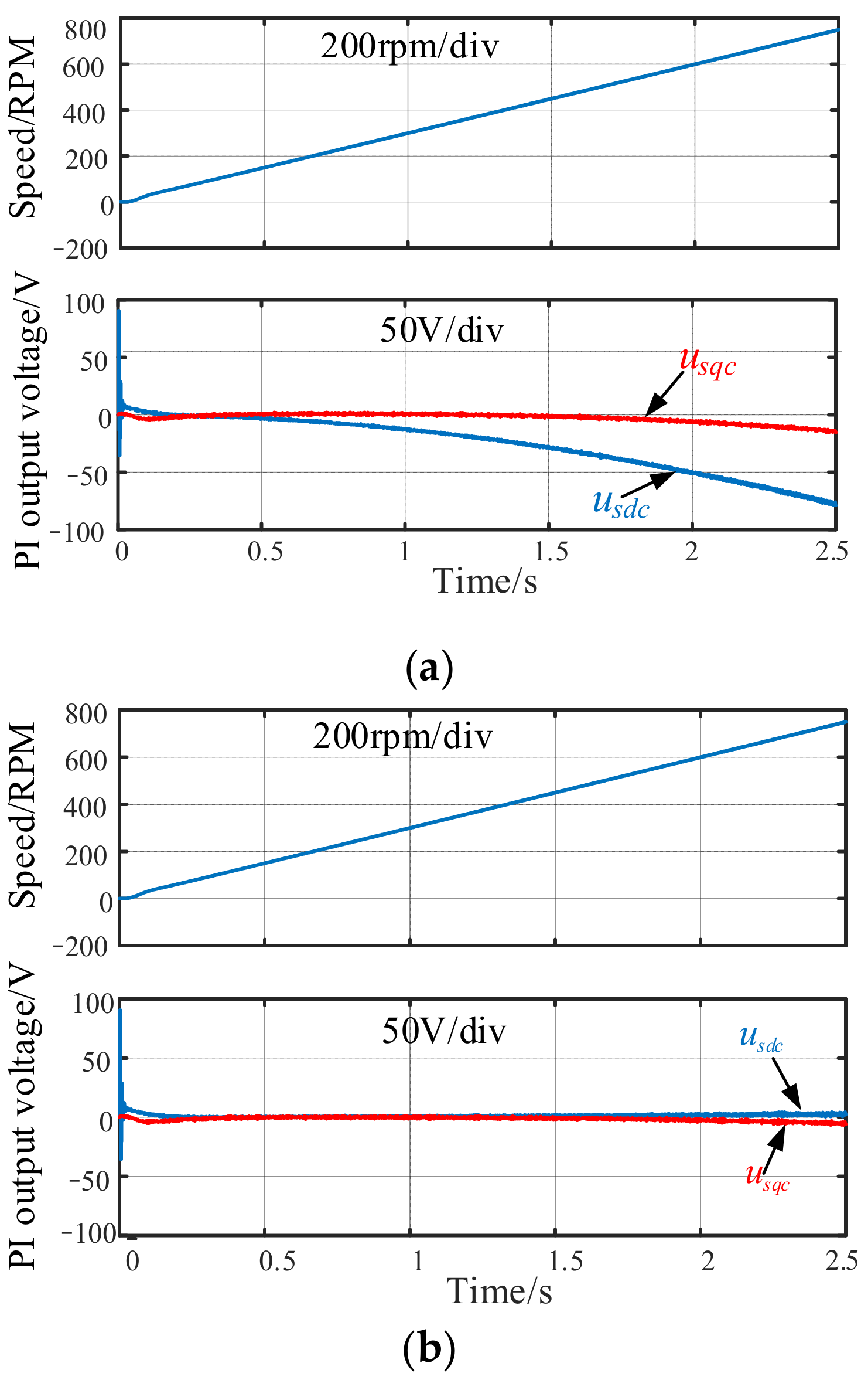
Affected by the delay, digitally controlled output voltage has specified phase lag and amplitude attenuation compared with the command voltage. This will further cause the output current amplitude attenuation and phase lag. Nevertheless, the inner current loop PI controller can adjust the amplitude and phase of the voltage vector command value so the voltage that can track its command well. That is to say, the current PI regulator compensates for the error of the voltage vector. Inspired by this, the PI controller’s outputs can be used to identify how large the error caused by the digital delay is.

Figure 16 shows the relationships of the output voltage commands of the current PI controller with regarding to the increase of the motor speed with/ without imposing the delay compensation strategy expressed in (28). In the figure, $u_{sdc}$ and $u_{sqc}$ are the d- and q-axis command components generated by the current PI controller. The larger the values of $u_{sdc}$, $u_{sqc}$ are, the more significant the voltage error caused by the delay is. Back to Figure 16a, the values get larger with the increase of the motor speed, indicating that the higher the speed is, the greater the output voltage error is. In contrast, after adopting the delay compensation strategy, both values remain near 0, as shown in Figure 16b. Hence, the delay compensation strategy adopted can effectively compensate for the voltage error caused by the digital delay.

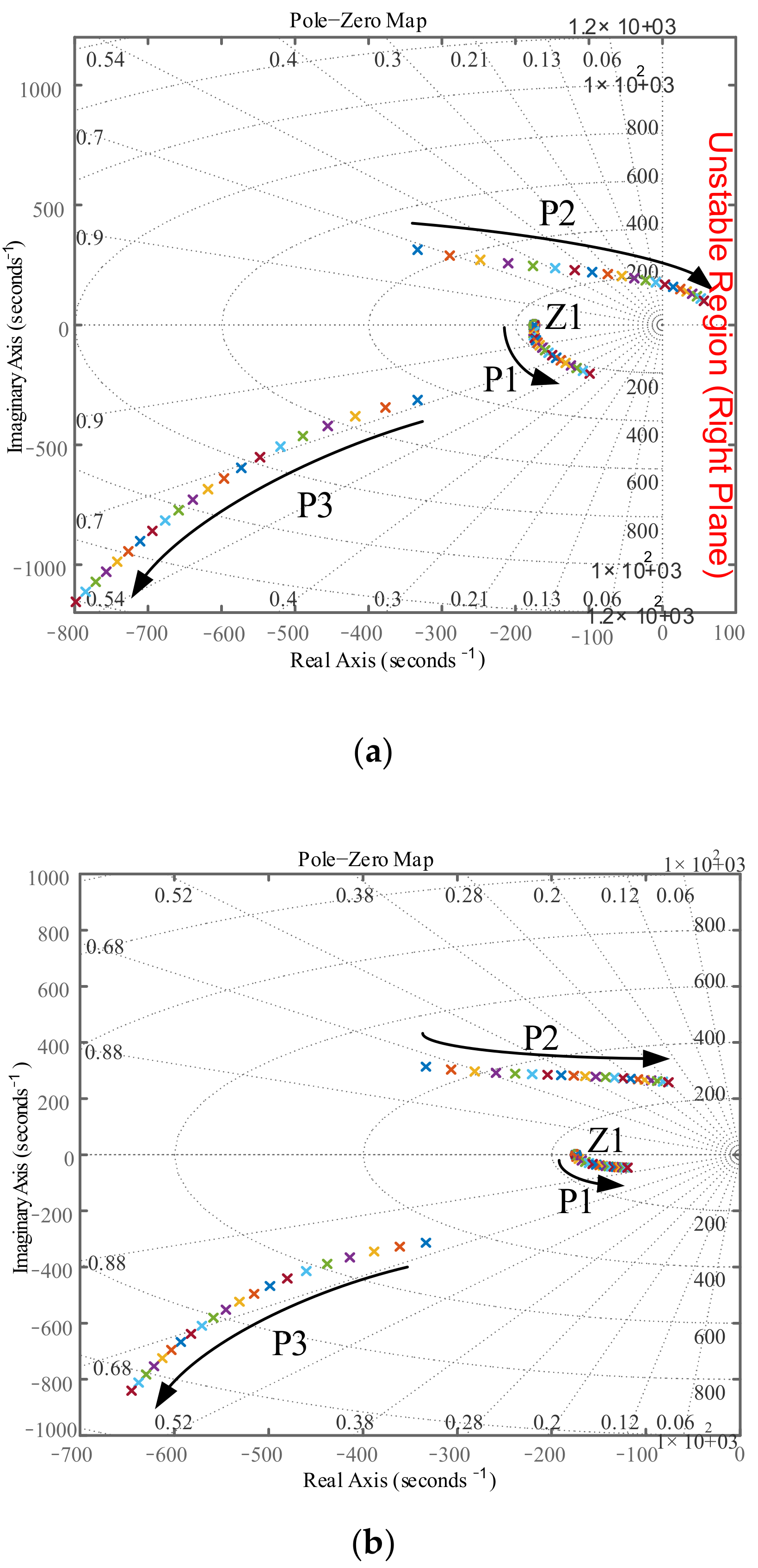
Further, Figure 17 shows the distribution of zero-pole points with/ without the delay compensation. It can be seen that before the delay compensation, some poles of the system will move to the unstable region (also the right plane of Pole-Zero Map) with the increase of synchronization frequency. In contrast, after compensating the delay, all poles are located in the left half plane. The system stability is therefore enhanced.

4.2. Improved Complex Vector Control

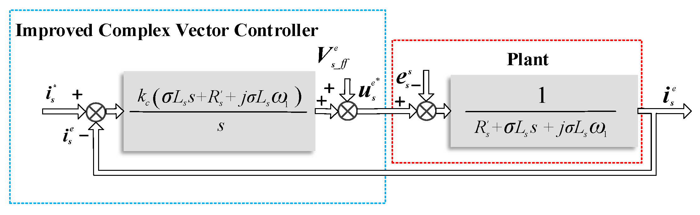
Using the delay compensation strategy to compensate for the digital control delay, the cross-coupling introduced by the digital delay can be well canceled. Thus, the control system is greatly simplified. According to the design idea of the complex vector current controller, using the zero-pole cancellation principle, the current controller can be designed in the following form:

$$G_c=\frac{k_c\left(\sigma L_{s}s+R_s^{\prime }+j\sigma L_s{\omega }_1\right)}{s}$$

(30)

Figure 18 shows the complex vector current control block diagram after delay compensation, in which the voltage compensation component ${\mathit{V}}_{\mathit{s}\_\mathit{f}\mathit{f}}^{\mathit{e}}$ is used to compensate the back-EMF coupling, and the complex vector controller is used to eliminate the control object coupling.

Thus, the closed-loop transfer function of the current loop becomes:

$$G_{clo}=\frac{{\mathit{i}}_{\mathit{s}}^{\mathit{e}}}{{\mathit{i}}_{\mathit{s}}^{\mathit{e}\ast }}=\frac{G_c{G}_p}{1+G_c{G}_p}=\frac{1}{s/k_c+1}$$

(31)

The system turns to be a real first-order inertial one, and the value of $k_c$ can be designed according to the bandwidth of the current loop. This decoupling method has strong parameter robustness of the control structure. Furthermore, it has the same form as the PI control (let $k_p=k_c·\sigma L_s$, $k_i=k_c·R_s^{\prime }$) while avoiding the complex PI tuning process.

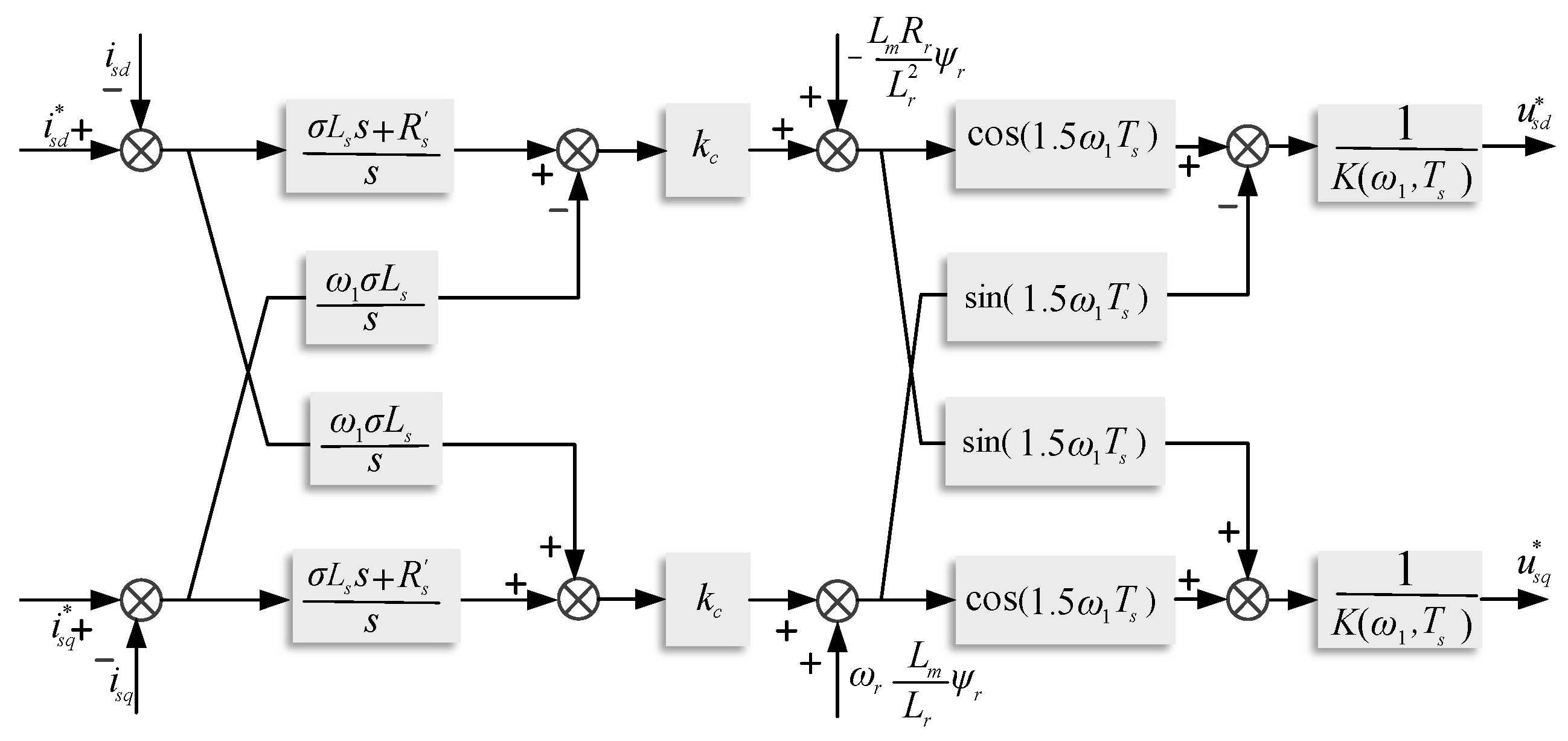
Figure 19 presents the scalar implementation loop for the proposed complex vector decoupling control. The proposed control uses offset current command value and the feed-back value of the voltage to build decoupling items. So, it achieves real-time adjustments of both feed-back and feed-forward decoupling.

5. Simulation and Experimental Verification

5.1. Simulation Results

In order to explore the performance of the proposed complex vector decoupling technique, the simulation on a MATLAB/Simulink platform is conducted. An induction motor drive system with the configuration shown in Figure 1 is applied in the simulation. Parameters of the system are summarized in

Table 1. Simulation and experimental parameters.

Symbol	Parameter	Value
Prated	Rated power	3000 W
Urated	Rated voltage	380 V
frated	Rated frequency	50 HZ
P	Pole count	3
RS	Stator resistance	11.8140 Ω
Rr	Rotor resistance	11.8429 Ω
LS	Stator leakage inductance	0.1835 H
Lr	Rotor leakage inductance	0.1835 H
Lm	Mutual inductance	0.1733 H
fSw	Switching frequency	500 Hz

.

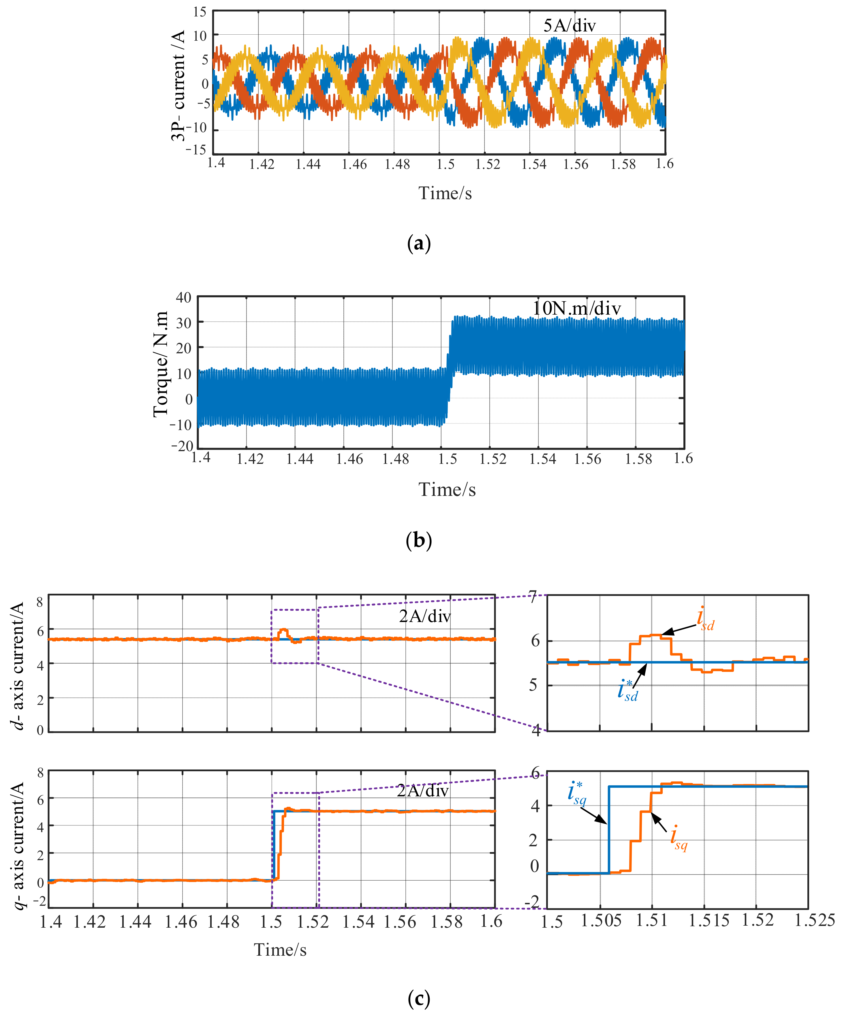
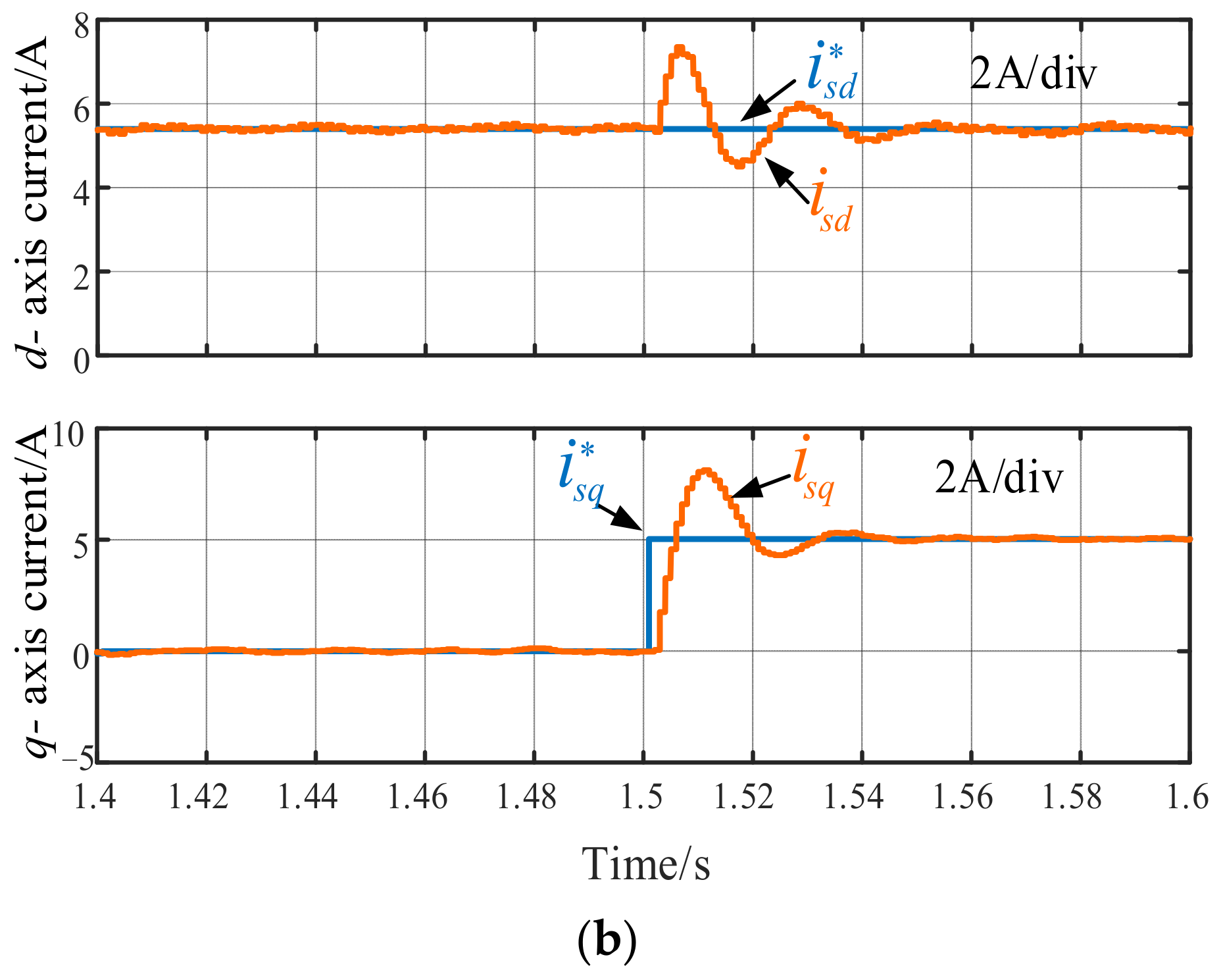
Figure 20 shows waveforms of the proposed decoupling with exact motor parameter values known in the control, i.e. $\widehat{\sigma }{\widehat{L}}_s=\sigma L_s$, and ${\widehat{R}}_s^{\prime }=R_s^{\prime }$, where $\widehat{\sigma }{\widehat{L}}_s$ and ${\widehat{R}}_s^{\prime }$ are estimation values used in the control. The waveforms from top to bottom are about three-phase currents, torque, d-axis current and q-axis current. As shown, when the q-axis current changes by step, the d-axis current is just slightly disturbed and then quickly recovers to its command value. The three-phase stator current and electromagnetic torque change steadily as well as the d-axis current. The above means the current coupling degree between d-axis and q-axis currents is significantly reduced.

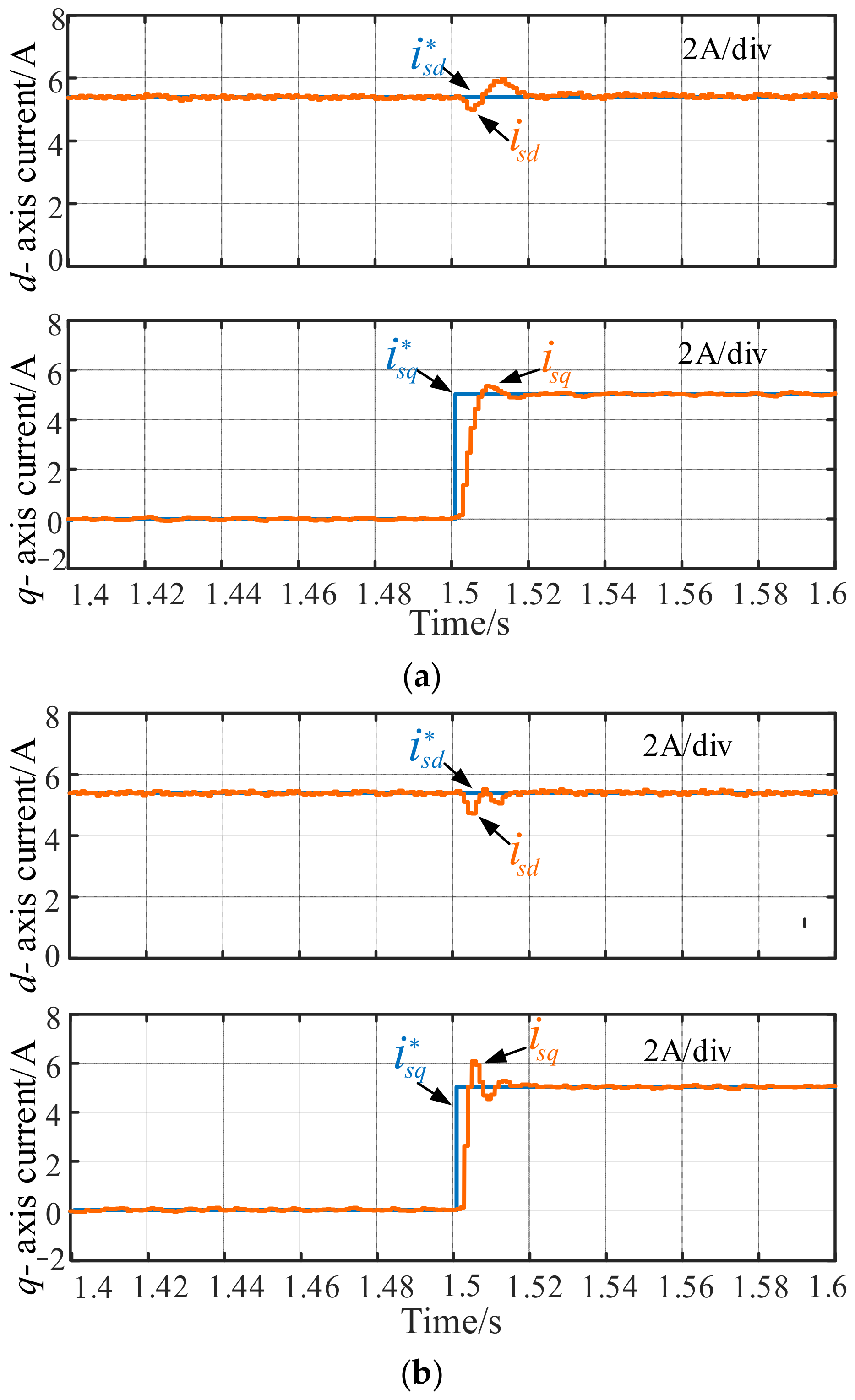
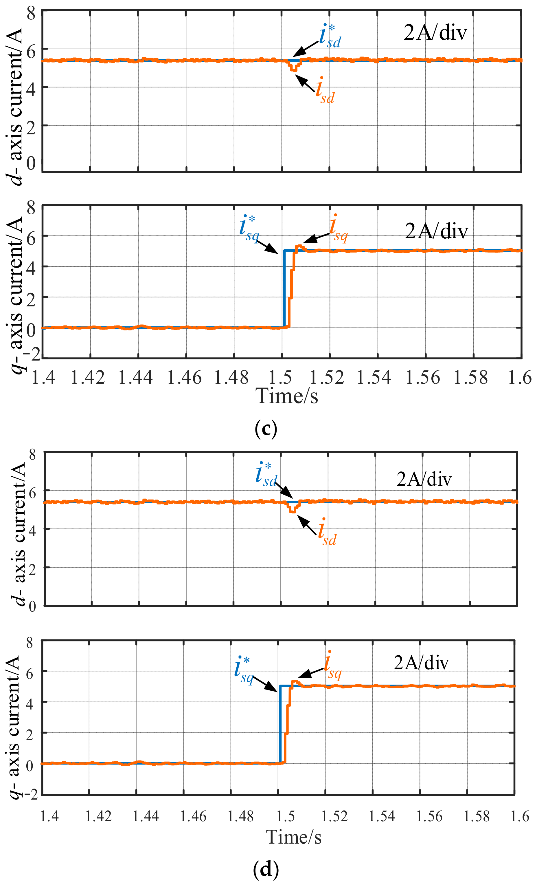
Note that, due to manufacturing differences and different environmental conditions, these IM parameter values have large or small errors with their practical values. Hence, it is very necessary to examine the parameter robustness using the proposed decoupling scheme. Consequently, four cases with reasonable parameter estimation errors are considered, i.e. $\widehat{\sigma }{\widehat{L}}_s=0.6\sigma L_s$$\widehat{\sigma }{\widehat{L}}_s=1.5\sigma L_s$, ${\widehat{R}}_s^{\prime }=0.6R_s^{\prime }$, and ${\widehat{R}}_s^{\prime }=1.5R_s^{\prime }$.

Figure 21a–d provide their corresponding dq-axis current response curves. No matter with any of the four cases, little difference can be observed compared with the accurate one in Figure 20a, which indicates these inaccurate parameter estimations do not affect the decoupling performance. Therefore, the decoupling control scheme proposed in this paper has considerable parameter robustness.

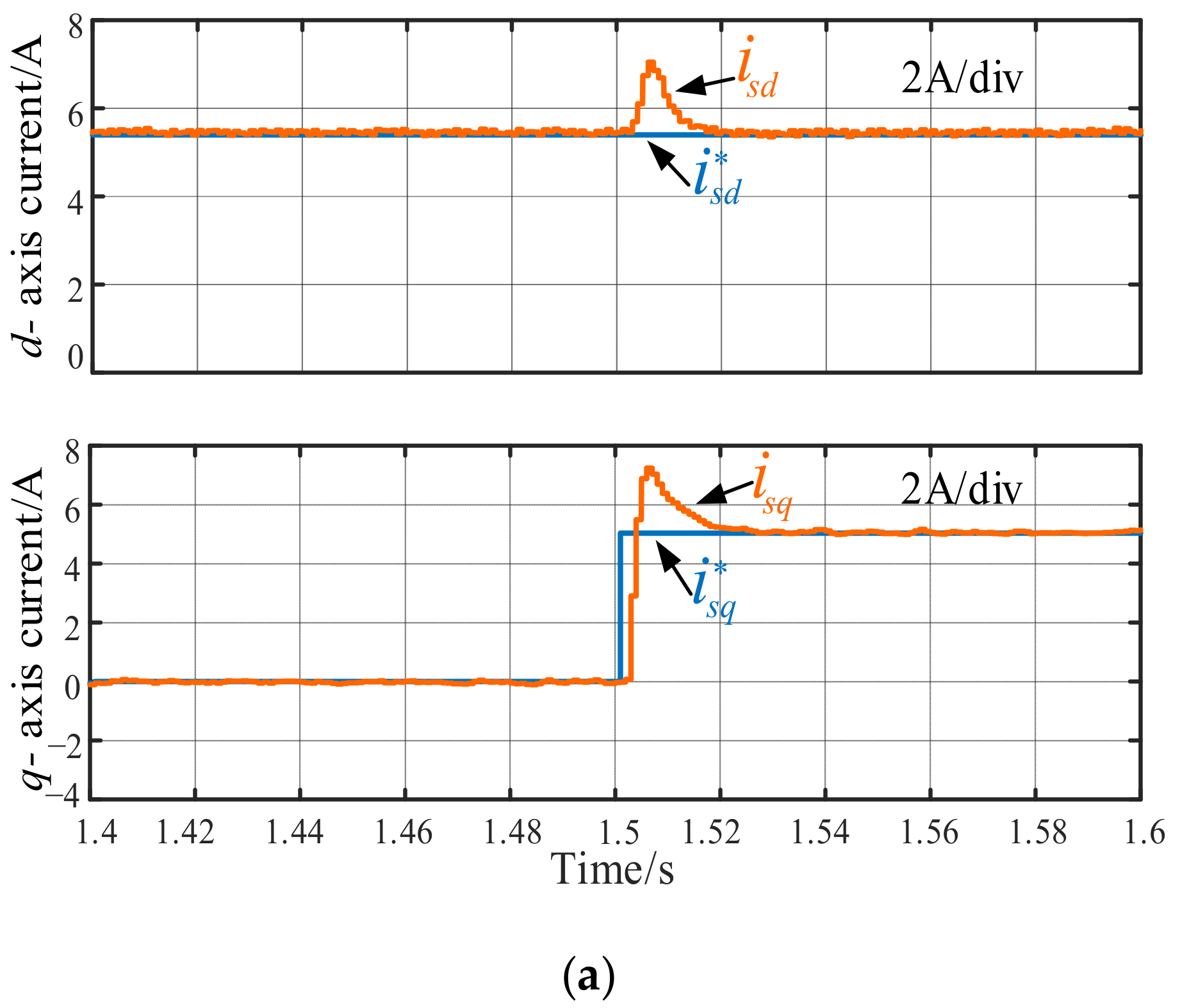
Figure 22 provides the comparison results between the feed-back decoupling and feed-forward decoupling. It can be seen that the feed-forward control shows better dynamic performance. Consequently, the feed-forward control is taken as the conventional representative to compare with our proposed scheme. The step response curves of the feed-forward decoupling control under accurate parameter conditions and estimated parameter error conditions (motor speed is 600 rpm) are provided in Figure 23. The coupling of d-q currents makes the transient d-axis current larger in the exact parameter condition than the estimated parameter error condition. The parameter robustness of feed-forward decoupling is not as good as the proposed scheme.

To further verify the validity of the proposed decoupling control, the comparison between the feed-forward decoupling control with delay compensation and the proposed complex vector controller is shown in Figure 24. After delay compensation, the coupling degree of feed-forward decoupling control is reduced to some degree. However, the degree is still high. In contrast, the proposed control shows much better decoupling performance. Till now, the parameter robustness and the decoupling effect of the proposed control is proved to be better than conventional ways.

5.2. Experimental Results

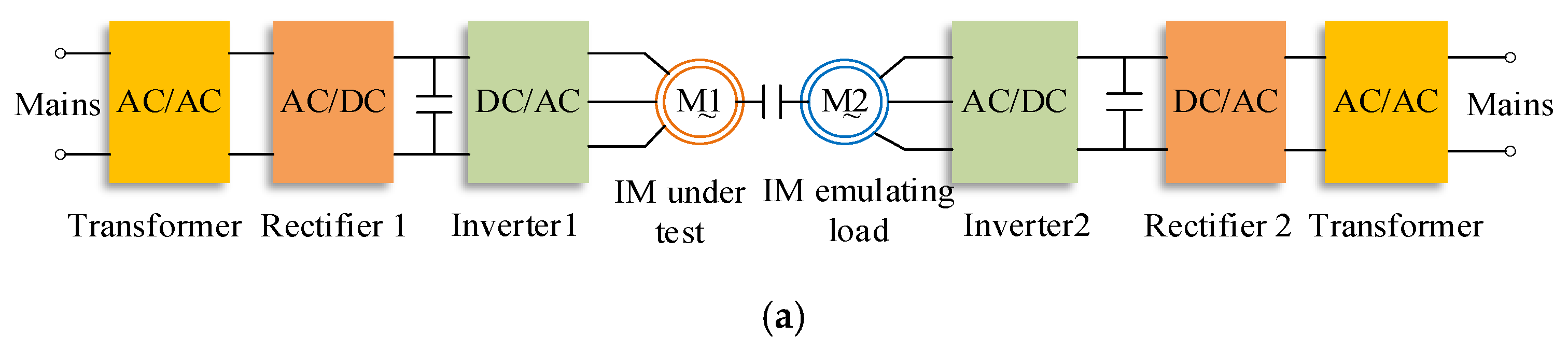
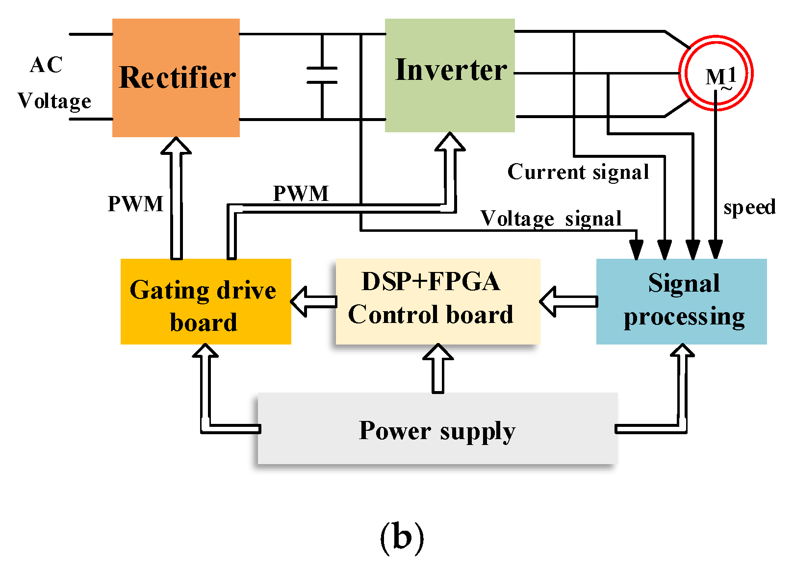
To investigate the effectiveness of the proposed control method, experiments were conducted with two 3 kW induction motors and their drive systems. Two inverter-motor systems are coaxially connected, as shown in Figure 25a. One IM (M1) serves as the motor under test. Another IM (M2) is used to emulate a load. Specifically, M2 stabilizes the speed at a constant value of 400 rpm. When the speed is stable, a command torque current of 5 A is suddenly added onto M1. Once the excitation current $i_{sq}$ reaches stable status, the torque current $i_{sd}$ changes from 0 A to 5 A in a step. Both drive systems are in a back-to-back configuration, as shown in Figure 25b and Figure 26. The Experiment parameters are the same as shown in Table 1.

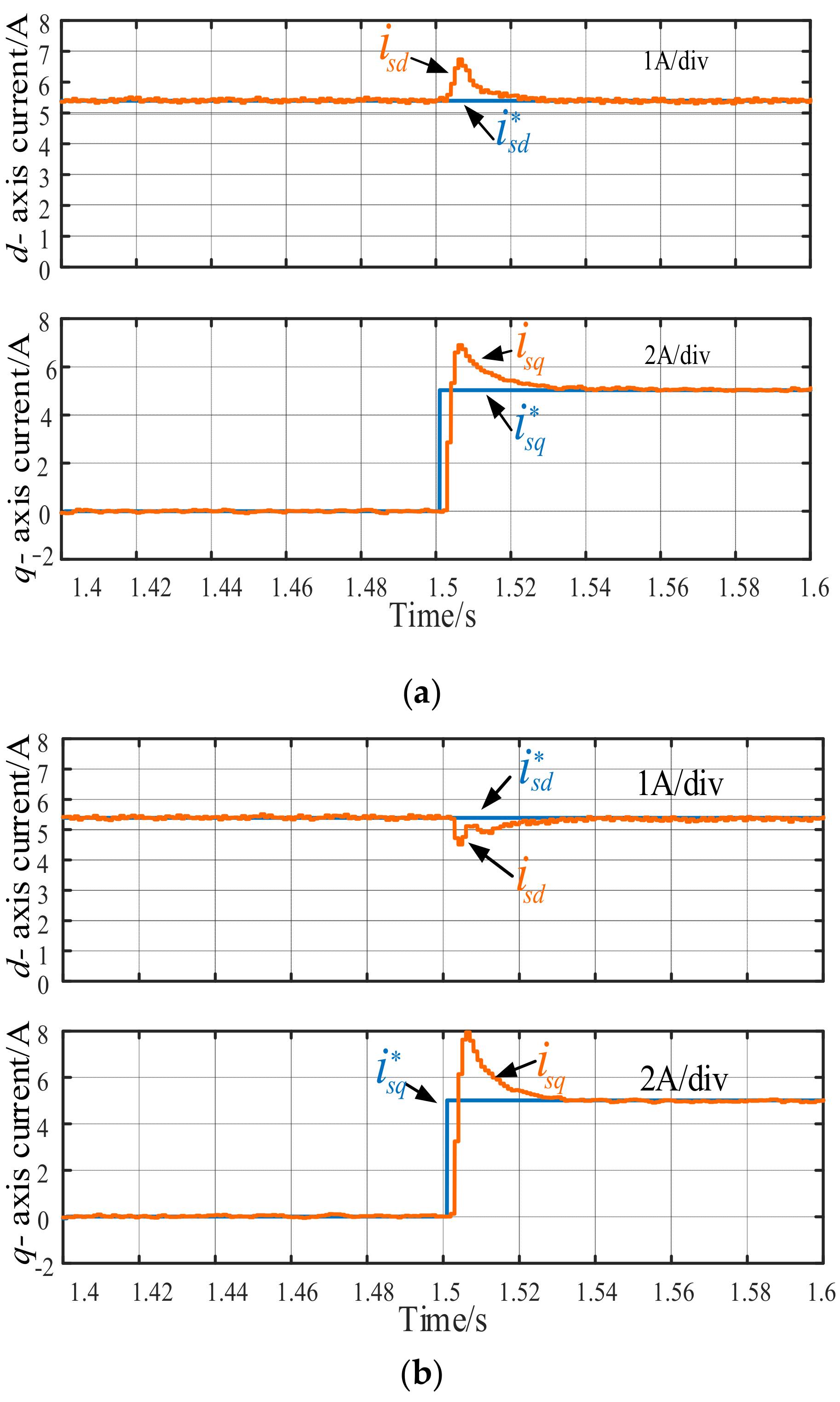
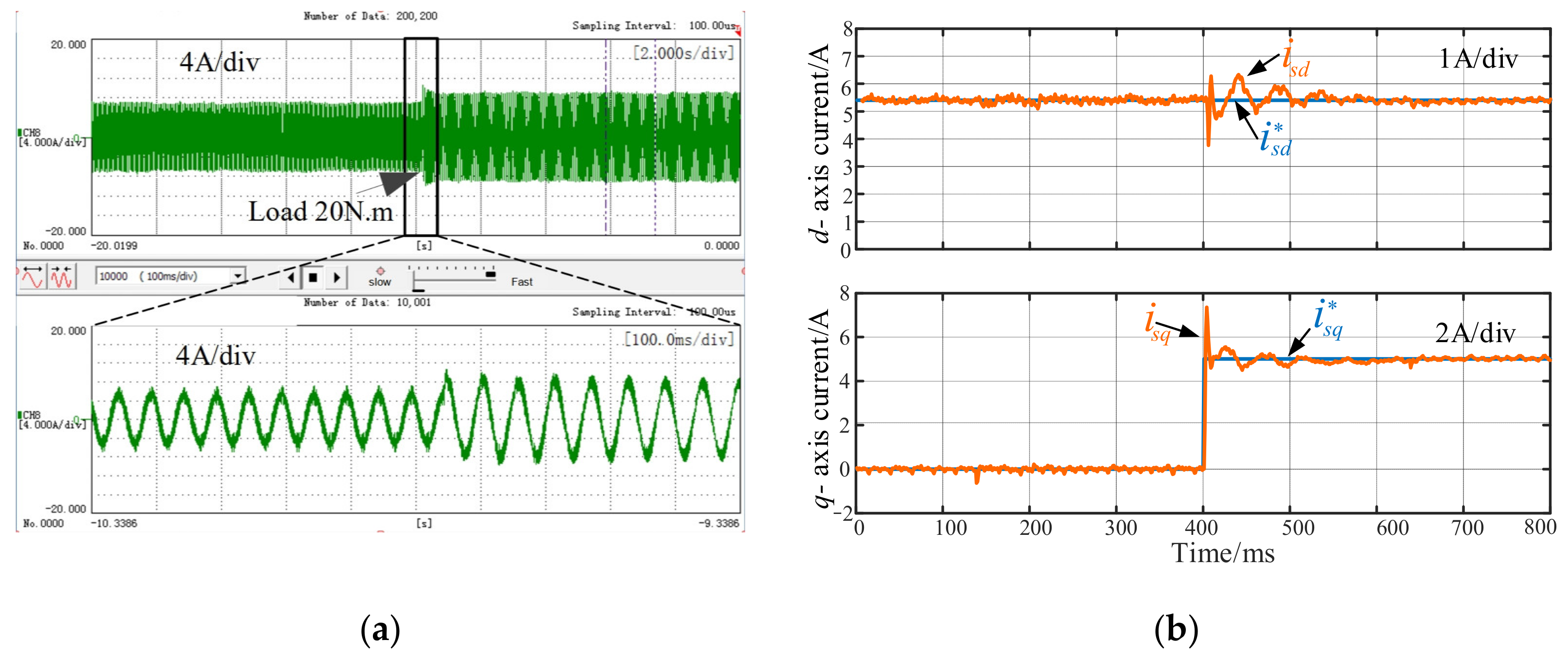
The PI control without decoupling and feed-forward decoupling control are shown in Figure 27 and Figure 28, respectively. Compared with the traditional PI control, when the q-axis current step changes, the amplitude of the current drop in the d-axis becomes smaller, indicating that the coupling degree is reduced to some extent for the feed-forward decoupling control.

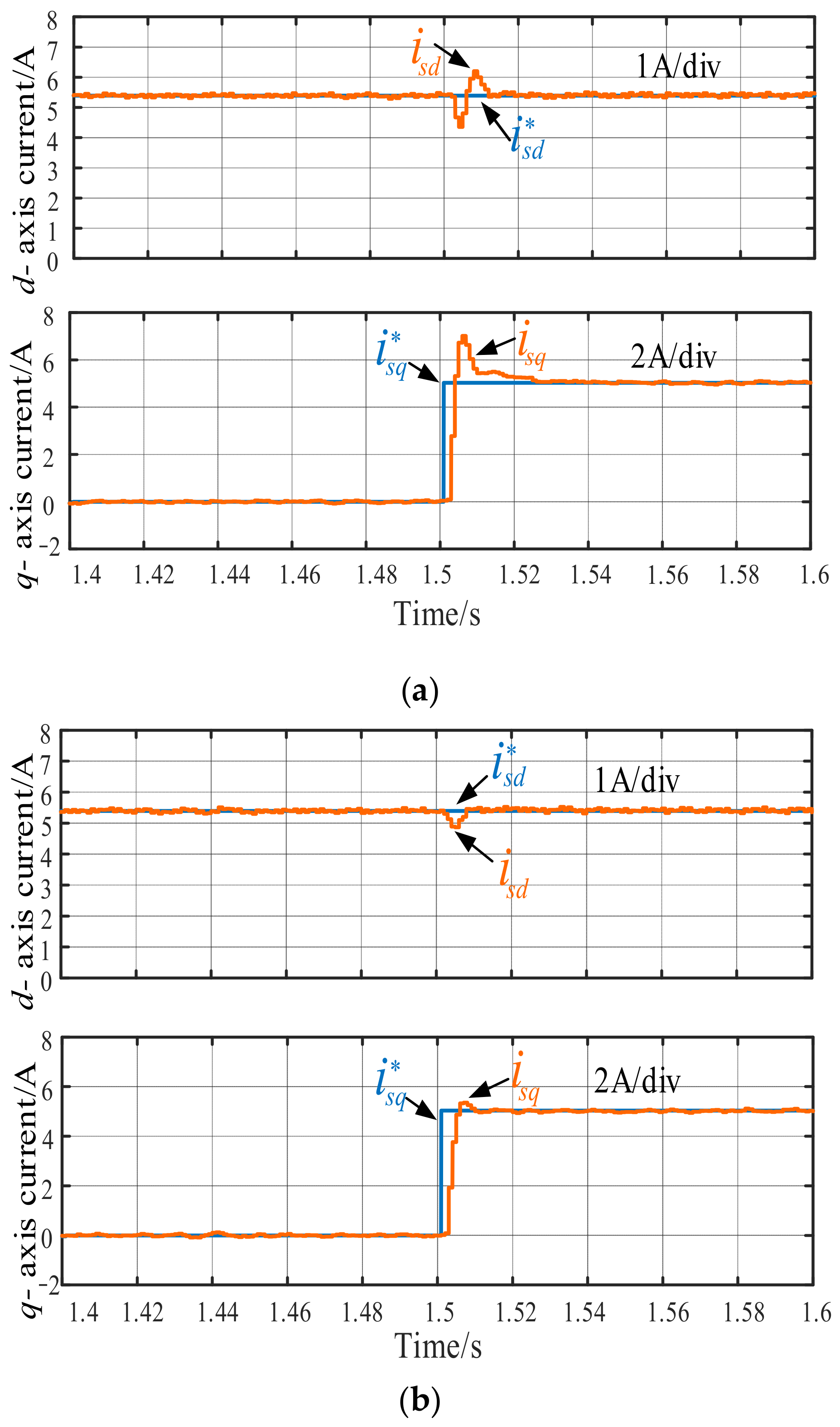
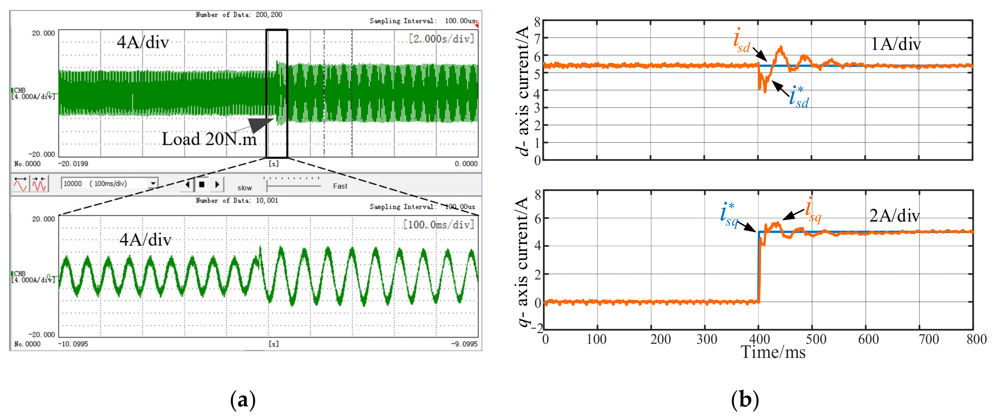
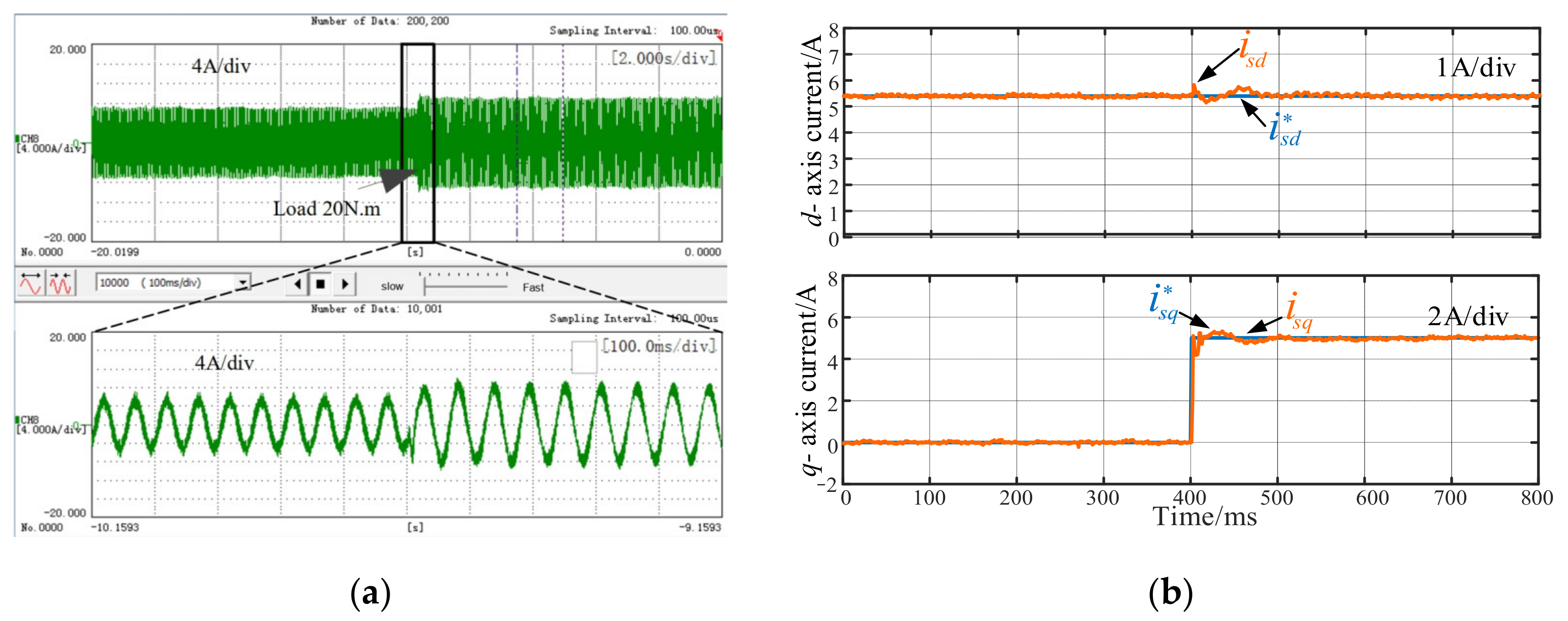
However, the q-axis current overshot is larger, indicating that the dq-axis current coupling is still serious. Finally, Figure 29 shows the experimental waveforms of the improved complex vector control scheme proposed in this paper. It can be seen that when the q-axis current step changes, the d-axis current is only slightly disturbed, and the command value is quickly tracked; there was no significant overshoot of the q-axis current either. Compared with the previous control schemes, the system response speed was faster, indicating that the complex vector control scheme has a better decoupling effect and better dynamic performance.

6. Conclusions

In this paper, a simple and effective complex vector decoupling is presented for the IM drive system at limited switching frequency conditions. In this method, the secondary effect on torque/flux coupling caused by digital control delay is specified and accurately compensated. Compared with the conventional PI current controller-based decoupling, it is immune to the digital delay and achieves optimized decoupling. Moreover, the dynamic component caused by the digital delay is canceled, which greatly simplifies the entire torque/flux decoupling process without compromising the system performance. Compared with the accurate-model-based complex vector control, the proposed decoupling has a simpler control structure and is easier to implement, making it more suitable for the actual industrial practice. The simulation and experimental results demonstrate that the decoupling control scheme proposed in this paper effectively improves the decoupling capability of the current loop and enhances the dynamic response, thus alleviating a good tradeoff between the system performance and implementation complexity.

References

- Matsuse, K.; Matsuhashi, D. New technical trends on adjustable speed AC motor drives. China J. Electron. Eng. 2017, 3, 1–9. [Google Scholar]
- Abouzeid, A.F.; Guerrero, J.M.; Endemaño, A.; Muniategui, I.; Ortega, D.; Larrazabal, I.; Briz, F. Control Strategies for Induction Motors in Railway Traction Applications. Energies 2020, 13, 700. [Google Scholar] [CrossRef] [Green Version]
- Kondo, M.; Miyabe, M.; Ebizuka, R.; Hanaoka, K. Design and Efficiency Evaluation of a High-Efficiency Induction Motor for Railway Traction. Electron. Eng. Jpn. 2015, 194, 15–23. [Google Scholar] [CrossRef]
- Mekrini, Z.; Seddik, B. Control of complex dynamical systems based on Direct Torque Control of an asynchronous machine. In Proceedings of the 2016 5th International Conference on Multimedia Computing and Systems (ICMCS), Marrakech, Morocco, 29 September–1 October 2016; pp. 537–542. [Google Scholar]
- Prieto, I.G.; Duran, M.J.; Garcia-Entrambasaguas, P.; Bermudez, M. Field-Oriented Control of Multiphase Drives With Passive Fault Tolerance. IEEE Trans. Ind. Electron. 2019, 67, 7228–7238. [Google Scholar] [CrossRef]
- Kumar, R.H.; Iqbal, A.; Lenin, N.C. Review of recent advancements of direct torque control in induction motor drives—A decade of progress. IET Power Electron. 2018, 11, 1–15. [Google Scholar] [CrossRef]
- El Moucary, C.; Mendes, E.; Razek, A. Decoupled direct control for PWM inverter-fed induction motor drives. IEEE Trans. Ind. Appl. 2002, 38, 1307–1315. [Google Scholar] [CrossRef]
- Wai, R.-J.; Lin, K.-M. Robust Decoupled Control of Direct Field-Oriented Induction Motor Drive. IEEE Trans. Ind. Electron. 2005, 52, 837–854. [Google Scholar] [CrossRef]
- Bahrani, B.; Kenzelmann, S.; Rufer, A. Multivariable-PI-Based dq Current Control of Voltage Source Converters With Superior Axis Decoupling Capability. IEEE Trans. Ind. Electron. 2010, 58, 3016–3026. [Google Scholar] [CrossRef]
- Bazzi, A.M.; Dominguez-Garcia, A.; Krein, P.T. Markov Reliability Modeling for Induction Motor Drives Under Field-Oriented Control. IEEE Trans. Power Electron. 2011, 27, 534–546. [Google Scholar] [CrossRef]
- Rodriguez, J.; Kennel, R.M.; Espinoza, J.R.; Trincado, M.; Silva, C.A.; Rojas, C.A. High-Performance Control Strategies for Electrical Drives: An Experimental Assessment. IEEE Trans. Ind. Electron. 2011, 59, 812–820. [Google Scholar] [CrossRef]
- Sergaki, E.S.; Essounbouli, N.; Kalaitzakis, K.C.; Stavrakakis, G.S. Fuzzy Logic Control for motor flux reduction during steady states and for flux recovery in transient states of Indirect-FOC AC drives. In Proceedings of the The XIX International Conference on Electrical Machines-ICEM 2010, Rome, Italy, 6–8 September 2010; pp. 1–6. [Google Scholar]
- Holmes, D.G.; McGrath, B.; Parker, S.G. Current Regulation Strategies for Vector-Controlled Induction Motor Drives. IEEE Trans. Ind. Electron. 2011, 59, 3680–3689. [Google Scholar] [CrossRef]
- Wang, K.; Ge, Q.; Li, Y.; Shi, L. An improved current regulation scheme used in indirect rotor field oriented control for AC traction applications. In Proceedings of the 2013 15th European Conference on Power Electronics and Applications (EPE), Lille, France, 2–6 September 2013; pp. 1–10. [Google Scholar]
- Shi, H.; Feng, Y.; Yu, X.; Li, L. Adaptive high-order terminal sliding modes control with decoupling stator current for induction motor. In Proceedings of the IECON 2011—37th Annual Conference of the IEEE Industrial Electronics Society, Victoria, Australia, 7–10 November 2011; pp. 3930–3935. [Google Scholar]
- Kommuri, S.K.; Rath, J.J.; Veluvolu, K.C.; Defoort, M.; Soh, Y.C. Decoupled current control and sensor fault detection with second-order sliding mode for induction motor. IET Control Theory Appl. 2015, 9, 608–617. [Google Scholar] [CrossRef] [Green Version]
- Wang, B.; Dong, Z.; Yu, Y.; Wang, G.; Xu, D. Static-Errorless Deadbeat Predictive Current Control Using Second-Order Sliding-Mode Disturbance Observer for Induction Machine Drives. IEEE Trans. Power Electron. 2017, 33, 2395–2403. [Google Scholar] [CrossRef]
- Zhou, S.; Liu, J.; Zhou, L.; Zhang, Y. DQ Current Control of Voltage Source Converters With a Decoupling Method Based on Preprocessed Reference Current Feed-forward. IEEE Trans. Power Electron. 2017, 32, 8904–8921. [Google Scholar] [CrossRef]
- Gobinath, D.; Vairaperumal, K.; Elamcheren, S. Simplified approach on feed forward vector control of induction motor with PI controller using SPWM technique. In Proceedings of the 2014 IEEE International Conference on Computational Intelligence and Computing Research, Coimbatore, India, 18–20 December 2014; pp. 1–4. [Google Scholar]
- Stojic, D.M.; Milinkovic, M.; Veinovic, S.; Klasnic, I. Stationary Frame Induction Motor Feed Forward Current Controller With Back EMF Compensation. IEEE Trans. Energy Convers. 2015, 30, 1356–1366. [Google Scholar] [CrossRef]
- Mon-Nzongo, D.L.; Ipoum-Ngome, P.G.; Flesch, R.C.; Song-Manguelle, J.; Jin, T.; Tang, J. Synchronous-frame decoupling current regulators for induction motor control in high-power drive systems: Modelling and design. IET Power Electron. 2020, 13, 669–679. [Google Scholar] [CrossRef]
- Ozturk, S.B.; Kivanc, O.C.; Atila, B.; Rehman, S.U.; Akin, B.; Toliyat, H.A. A simple least squares approach for low speed performance analysis of indirect FOC induction motor drive using low-resolution position sensor. In Proceedings of the 2017 IEEE International Electric Machines and Drives Conference (IEMDC), Miami, FL, USA, 21–24 May 2017; pp. 1–8. [Google Scholar]
- He, L.; Xiong, J.; Ouyang, H.; Zhang, P.; Zhang, K. High-Performance Indirect Current Control Scheme for Railway Traction Four-Quadrant Converters. IEEE Trans. Ind. Electron. 2014, 61, 6645–6654. [Google Scholar] [CrossRef]
- Li, Q.; Jiang, D.; Zhang, Y.; Liu, Z. The Impact of VSFPWM on DQ Current Control and a Compensation Method. IEEE Trans. Power Electron. 2020, 36, 3563–3572. [Google Scholar] [CrossRef]
- Bae, B.-H.; Sul, S.-K. A compensation method for time delay of full-digital synchronous frame current regulator of pwm ac drives. IEEE Trans. Ind. Appl. 2003, 39, 802–810. [Google Scholar] [CrossRef]
- Yepes, A.G.; Vidal, A.; Malvar, J.; Lopez, O.; Doval-Gandoy, J. Tuning Method Aimed at Optimized Settling Time and Overshoot for Synchronous Proportional-Integral Current Control in Electric Machines. IEEE Trans. Power Electron. 2013, 29, 3041–3054. [Google Scholar] [CrossRef]
- Kim, H.; Degner, M.; Guerrero, J.M.; Briz, F.; Lorenz, R.D. Discrete-Time Current Regulator Design for AC Machine Drives. IEEE Trans. Ind. Appl. 2010, 46, 1425–1435. [Google Scholar] [CrossRef]
- Diao, L.-J.; Sun, D.-N.; Dong, K.; Zhao, L.-T.; Liu, Z.-G. Optimized Design of Discrete Traction Induction Motor Model at Low-Switching Frequency. IEEE Trans. Power Electron. 2012, 28, 4803–4810. [Google Scholar] [CrossRef]
- Wang, Y.; Tobayashi, S.; Lorenz, R.D. A Low-Switching-Frequency Flux Observer and Torque Model of Deadbeat–Direct Torque and Flux Control on Induction Machine Drives. IEEE Trans. Ind. Appl. 2014, 51, 2255–2267. [Google Scholar] [CrossRef]
- Briz, F.; Díaz-Reigosa, D.; Degner, M.W.; García, P.; Guerrero, J.M. Current sampling and measurement in PWM operated AC drives and power converters. In Proceedings of the 2010 International Power Electronics Conference—ECCE ASIA, Sapporo, Japan, 21–24 June 2010; pp. 2753–2760. [Google Scholar]
- Chen, C.; Xiong, J.; Wan, Z.; Lei, J.; Zhang, K. A Time Delay Compensation Method Based on Area Equivalence For Active Damping of an LCL-Type Converter. IEEE Trans. Power Electron. 2016, 32, 762–772. [Google Scholar] [CrossRef]
Figure 1.
Control block diagram of Flux Oriented Control system.
Figure 2.
Complex vector signal flow diagram of induction motor in dq coordinate system.
Figure 3.
The digital timing diagram for the current control loop.
Figure 4.
Time delay caused by the asymmetry sampling.
Figure 5.
Voltage complex vector expressions in different coordinate frames.
Figure 6.
Coupling effect of digital control delay in the stationary/synchronous frame.
Figure 7.
Feed-forward current controller block diagram.
Figure 8.
Closed-loop pole-zero map of feed-forward decoupling control.
Figure 9.
Feed-back decoupling control block diagram.
Figure 10.
Closed-loop pole-zero map of feed-back decoupling control.