The Control Method of Twin Delayed Deep Deterministic Policy Gradient with Rebirth Mechanism to Multi-DOF Manipulator

Abstract

As a research hotspot in the field of artificial intelligence, the application of deep reinforcement learning to the learning of the motion ability of a manipulator can help to improve the learning of the motion ability of a manipulator without a kinematic model. To suppress the overestimation bias of values in Deep Deterministic Policy Gradient (DDPG) networks, the Twin Delayed Deep Deterministic Policy Gradient (TD3) was proposed. This paper further suppresses the overestimation bias of values for multi-degree of freedom (DOF) manipulator learning based on deep reinforcement learning. Twin Delayed Deep Deterministic Policy Gradient with Rebirth Mechanism (RTD3) was proposed. The experimental results show that RTD3 applied to multi degree freedom manipulators is in place, with an improved learning ability by 29.15% on the basis of TD3. In this paper, a step-by-step reward function is proposed specifically for the learning and innovation of the multi degree of freedom manipulator’s motion ability. The view of continuous decision-making and process problem is used to guide the learning of the manipulator, and the learning efficiency is improved by optimizing the playback of experience. In order to measure the point-to-point position motion ability of a manipulator, a new evaluation index based on the characteristics of the continuous decision process problem, energy efficiency distance, is presented in this paper, which can evaluate the learning quality of the manipulator motion ability by a more comprehensive and fair evaluation algorithm.

1. Introduction

Deep reinforcement learning (DRL) is a research hotspot in the field of artificial intelligence. In 2015, its landmark achievement, deep Q learning, was published in Nature [1]. At present, DRL is a general form of artificial intelligence learning. Its advantage is that it combines the perception ability of deep learning (DL) with the decision-making ability of reinforcement learning (RL), and realizes the direct control from the original input to the output through the end-to-end learning [2]. The basic idea of deep learning is to form abstract high-level features by extracting low-level features through multi layer network structure and nonlinear transformation, so as to represent the distributed features of data [3]. The basic idea of RL is to get the highest cumulative reward value through the interaction between agent and environment, so as to get the optimal strategy to complete the task [4]. As hot issues in the field of artificial intelligence, they have shown their unique advantages in helping human beings solve complex practical problems. Deepmind, a research team of Google, combines the abstract representation ability of deep learning with the problem-making ability of reinforcement learning, forming a new research hotspot in the field of artificial intelligence-DRL.

The multi-degree of freedom (DOF) manipulator is used in industrial applications because of its flexibility to achieve high motion capacity. Traditional manipulator motion planning is based on the known kinematics model of the manipulator. The most classical method to establish the kinematics model is the D-H parameter method proposed by Denavit and Hartenberg [5]. When the position of the end of the manipulator is known, the key to successful completion of the task is to get the inverse kinematics solution of the rotation angle of each joint of the manipulator [6]. Traditional inverse kinematics solution methods include analytical and numerical methods [7]. However, the analytical method is not suitable for solving multi joint manipulators with complex structures, and the numerical method of iterative evaluation is not suitable for real-time control of manipulators [8]. When completing the task of reaching the target position with the end-effector of the manipulator, the accuracy of reaching target position depends on the modeling accuracy of the kinematics model of the manipulator. In general, there are two necessary conditions for the manipulator to plan its kinematics capability with the known kinematics model. Even if the working environment is known, all modern manipulators use closed loop control, based on kinematic or dynamic model. The position accuracy that a manipulator can reach depends on the accuracy of its own kinematics model and the measurement accuracy of the position it reaches. Second, the nature of the task is mostly static, that is, when the base and target position of the manipulator are relatively static, the manipulator uses the kinematics model to plan the motion to reach the target position.

Many researchers are seeking for solutions in many different areas, as well as a way to break through the current limitations through different areas. As an important resource in modern society, data has also become an important factor to promote the development of control theory. Roman et al. [9] used a 3DOF tower crane to verify the effectiveness of the hybrid data-driven fuzzy active disturbance rejection control(ADRC) algorithms and this algorithms are validated as controllers in terms of real-time experiments. Haibo et al. [10] used data-driven technology to build an intelligent transportation system based on modern control principles.Research on model-based control methods is also meaningful.Based on the accurate flexible system model, Timothy Sands designed a whiplash compensator [11]. The compensator is very suitable for flexible multibody system. This paper is also dedicated to the application of DRL theory to multi-DOF manipulators, and combines bionic technology with DRL to establish a model-free multi-DOF manipulator motion control.

DRL is a form of effective learning in high-dimensional problems that cannot be solved by traditional robotic motion technology [12]. By experiment and exploration, reward and punishment, memory and update constantly refining skill levels, high levels of knowledge and skills can be obtained. In many explorations and attempts to use deep reinforcement learning to help the manipulator learn its motion ability, many teams have gained some useful experience and knowledge. At present, most of the team’s research on deep reinforcement learning applied to the manipulator focuses on three aspects: first, due to the sparse reward problem, it is difficult for the agent to get reward under the initialization strategy, which leads to training difficulties [13], so it is necessary to design a reward function that is closer to the learning characteristics of the manipulator [14]; second, in order to improve the learning efficiency of the manipulator, various experience playback mechanisms are put forward after updating and optimizing the experience pool in the RL. New and optimized, put forward various experience playback mechanisms to improve the learning efficiency of the manipulator [15]; third, the innovational modification in network structure brings improvement, which makes the motion ability learning for high-dimensional complexity manipulator possible [16].

Kwiatkowsk et al. used DL methods to make the manipulator build self-model [17]. At first the manipulator did not know its shape and joint connection, but after 35 h of training, it was able to build a self-model with little error from the actual physical model. Levine et al. proposed a monocular vision-based hand-eye coordination method for the capture task of a manipulator. This method trains a convolution neural network, which relies on the image information collected by a real-time camera and the current status of the manipulator to learn the skills of case coordination, and uses fourteen actual manipulators to collect 800,000 attempts in two months to make the manipulator obtains grabbing ability [18]. Ichnowski et al. proposed a warm-start optimizing motion planner based on DL to reduce computation and movement time [19]. However, these beneficial attempts are generally inefficient and take longer time to train. Fujimoto et al. improved the DDPG algorithm to reduce the overestimation bias of value, proposed the Twin Delayed Deep Deterministic Policy Gradient(TD3) algorithm, and verified the TD3 algorithm’s ability through experiments [20]. Qian et al. of King’s College London combined an updated version of DDPG-TD3 with an adaptive neuro-fuzzy proportion integral derivative(PID) controller to optimize control performance, using TD3 to generate multiple parameters of the fuzzy PID controller [21]. Andrs Antos suggests that when applying reinforcement learning algorithms to time-bounded continuous decision space problems, a strategy search step, such as the Actor-Critic algorithm, is required [22]. These results show that the TD3 algorithm is suitable for solving the problem of the manipulator’s motion capability in high-dimensional continuous decision space [23]. Google Brain’s OT-Opt research has yielded a very surprising result. By using end-to-end training to control the real manipulator to grab objects in an deep learning system, Google’s researchers combined large-scale distributed optimization with a new deep learning algorithm and proposed a new algorithm called OT-Opt. The reward function is designed as follows: if the end-effector of the manipulator successfully grabs an object from the box, it gets a reward value of 1; otherwise, it gets a reward value of 0 [24]. For the sparse reward problem, Lui et al. helped the manipulator learn the ability to reach the target position by optimizing the reward function [25]. Because these studies only used the result information as the basis for reward function design, they ignored the problem that the manipulator reached the target position as a process problem.

The structure of this paper is as follows: the first part introduces the related content of deep reinforcement learning and the research status of multi-DOF manipulator control; the second part introduces the problems to be solved and the main methods to be adopted in this paper; the third part introduces the design of step-by-step reward function proposed in this paper in detail; the fourth part introduces the design of rebirth mechanism and RTD3 algorithm proposed in this paper in detail structure; the fifth part introduces the evaluation index of intelligent algorithm proposed in this paper; the sixth part describes the experimental design in detail, shows the results and discusses the experimental results; the seventh part evaluates the experimental results, analyzes the advantages and disadvantages of the experiment, and prospects the future research direction.

2. Related Work

This paper will further improve the training efficiency through two aspects. These two aspects are: one is to design a new deep reinforcement learning network structure based on TD3; the other is to design a new reward function ‘step-by-step reward function’. Therefore, this paper will improve the network structure of the TD3 algorithm for better learning of the manipulator’s motion capability, further suppress the overestimation bias of Q value, and propose a new Twin Delayed Deep Deterministic Policy Gradient with Rebirth Mechanism (RTD3) algorithm. Since the previous reward function design did not overcome the sparse reward problem well, so the multi-DOF manipulator can not better use the DRL method to obtain better motion ability. In this paper, a new reward function, step-by-step reward function, is proposed to learn the motion ability of a manipulator faster and better. The reward function evaluates each step of the manipulator motion by treating the manipulator motion as a continuous decision-making problem, which enables the manipulator to achieve a higher mobility.

Unlike previous reward scores to evaluate the learning effect of a manipulator’s motor ability, this paper presents a new criterion, the efficienct distance, as an index to measure the motion ability of a manipulator, which is based on the continuous decision-making process problem.

Firstly, the motion problem of multi-DOF Manipulator is decomposed into Markov decision process (MDP). The MDP is a mathematical model of sequential decision, which is used to simulate the randomness strategies and returns that an agent can achieve in an environment where the system state has Markovian properties [4,26]. MDP is built on a set of interactive objects, that is, agents and environments, with elements including status, actions, strategies, and rewards [26].

In this paper, the 3DOF manipulator is used as an agent of machine learning in MDP to perceive the external environment and make action decisions, and adjust the decisions through the feedback of the environment. The process of decomposing the learning of motion capability of a 3DOF manipulator into MDP is illustrated as

Table 1. Markov decision process.

Name	Symbolism	Explanation
State	$S=\{s_1,s_2,\dots ,s_T\}$	State space refers to the workspace of a manipulator and is an environment composed of continuous spatial position coordinates.
Action	$A=\{a_1,a_2,\dots ,a_T\}$	Motion is the angular increment command issued by the three corresponding joints of the manipulator arm. The action space is continuous.
Policy	$\pi \left(a\right|s)=p(a\left|s\right)$	Actions given by status.
Reward	$R=R(s_t,a_t,s_{t+1})$	When the arm moves, it is rewarded for reaching the target position, that is, the environment’s feedback to the agent.
Return	$G=\sum R_i$	Return is the accumulation of rewards over step time.

.

3. Step-by-Step Reward Function

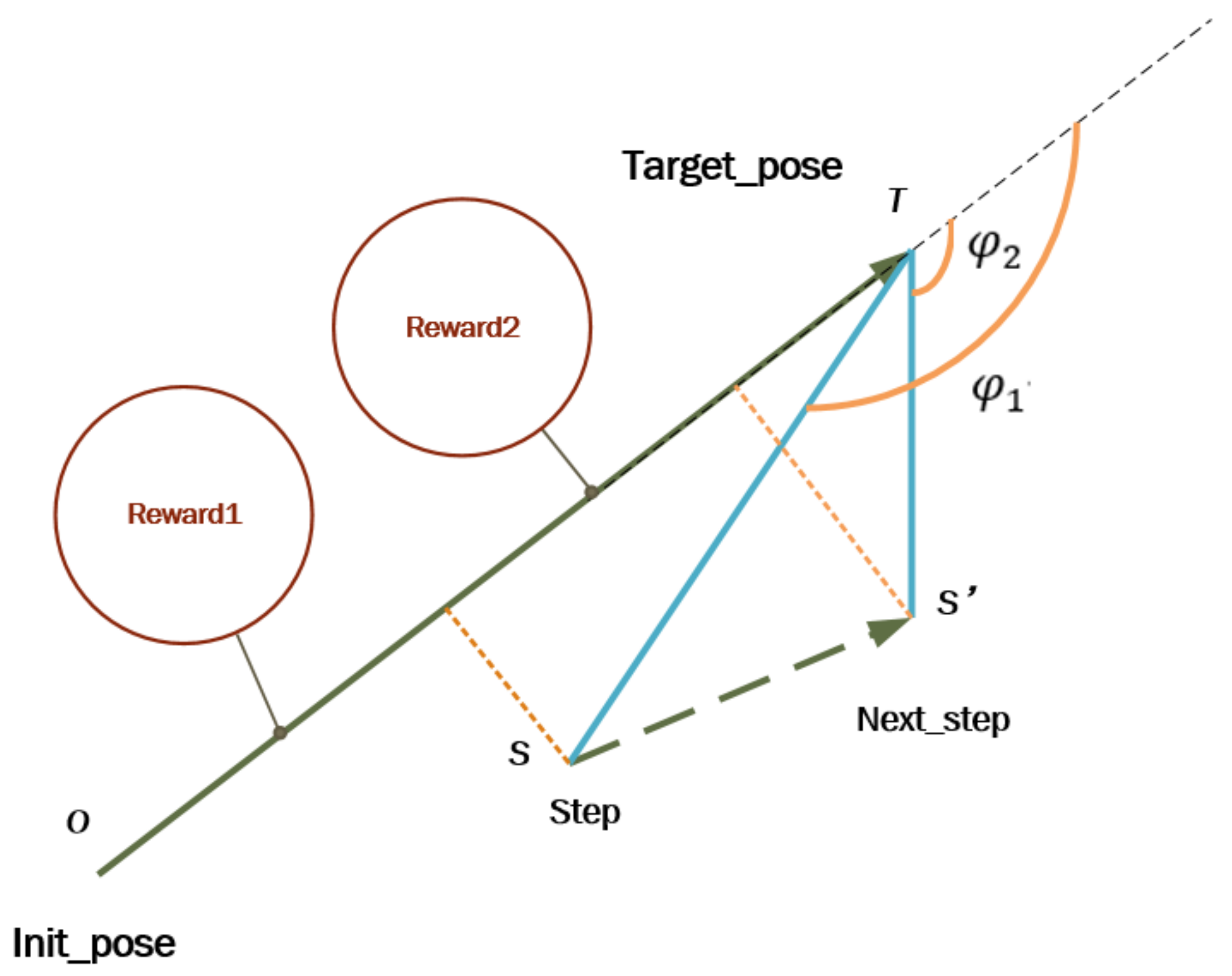
The design of the step-by-step reward function is based on the sparse reward problem and the learning ability of the manipulator. The sparse reward problem does not work well in solving continuous decision-making problems. The problem with sparse rewards is that there is a portion of the learning vacuum between being punished and being rewarded due to the discontinuity of rewards. When the manipulator is learning in this part of the learning vacuum area, it is blind and useless to spend most of its time and energy. Therefore, the sparse reward problem will cause the slow convergence of the network and the poor learning efficiency of the manipulator’s motion ability. At present, many reward functions have been designed to solve the sparse reward problem as a process problem to achieve better learning results, such as distance reward function, azimuth reward function and so on. The advantage of the reward function designed in this paper is that the process of reaching the target position of the manipulator is taken as the basis for the design of the reward function. In the design of step-by-step reward function, the positive and negative reward values are given separately for each step of the task according to the principle that effective results are encouraged. The step-by-step reward function is designed to consider the projection of the end-effector position of the manipulator on the spatial vector from the starting position to the target position, near or far from the target position, and to use the projection as the criterion to get the reward value. The calculation principle is shown in Figure 1.

The distance from the current position at the end-effector of manipulator to the target position is $L_{reward1}$, and $L_{reward1}$ is given as:

$$L_{reward1}=\left|\overrightarrow{ST}\right|.$$

(1)

The first part of the step-by-step reward function is $R_{reward1}$ as follows:

$$R_{reward1}=-{\lambda }_1{L}_{reward1},{\lambda }_1\in (0,+\infty ),$$

(2)

where $L_{reward2}$ is stepped distance as Equation (3), which could represent the effect of $\overrightarrow{S{S}^{\prime }}$ approaching the target in the current step.

$$L_{reward2}=\frac{\overrightarrow{OT}·\overrightarrow{S{S}^{\prime }}}{|\overrightarrow{OT}|}$$

(3)

Through the comparison of ${\phi }_1$ and ${\phi }_2$, the positive or negative effects of the current manipulator motion step is determined. ${\phi }_1$ and ${\phi }_2$ are defined as follows:

$${\phi }_1=\frac{\overrightarrow{OT}·\overrightarrow{TS}}{|\overrightarrow{OT}|·|\overrightarrow{TS}|},$$

(4)

$${\phi }_2=\frac{\overrightarrow{OT}·\overrightarrow{T{S}^{\prime }}}{|\overrightarrow{OT}|·|\overrightarrow{T{S}^{\prime }}|}.$$

(5)

The second part of the step-by-step reward function is $R_{reward2}$ as Equation (6).

$$R_{reward2}={\lambda }_2{L}_{reward2}$$

(6)

The step-by-step reward function R is defined as:

$$R=R_{reward1}+R_{reward2}.$$

(7)

where ${\lambda }_1$ is a normal number and is the gain coefficient for the first part of the reward. ${\lambda }_2$ is the gain coefficient for the second part of the reward, which is discussed in six cases.

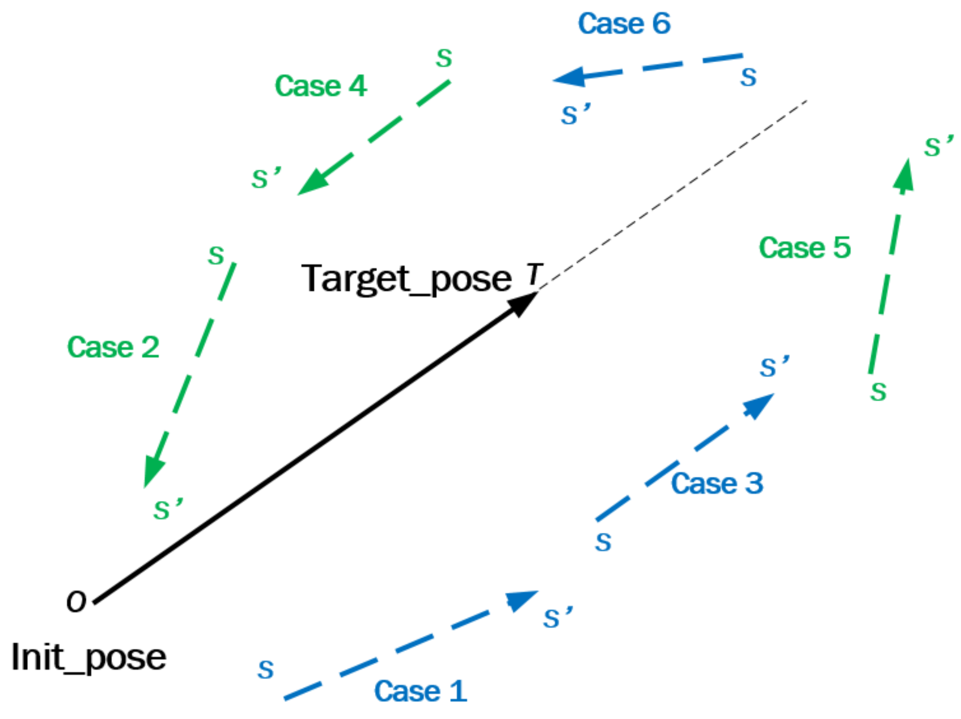
The movement process of the manipulator’s end-effector from the initial position to the target position is classified into six cases. As shown in Figure 2, through the analysis of the six cases, the six cases are divided into two categories: the proximity to get positive reward and the distance to get negative reward.

$$case1:\frac{\pi }{2}<{\phi }_2<{\phi }_1,$$

(8)

$$case2:\frac{\pi }{2}<{\phi }_1<{\phi }_2,$$

(9)

$$case3:{\phi }_2<\frac{\pi }{2}<{\phi }_1,$$

(10)

$$case4:{\phi }_1<\frac{\pi }{2}<{\phi }_2,$$

(11)

$$case5:{\phi }_2<{\phi }_1<\frac{\pi }{2},$$

(12)

$$case6:{\phi }_1<{\phi }_2<\frac{\pi }{2}.$$

(13)

Six cases are analyzed and divided into two categories. Corresponding to the two cases, ${\lambda }_2$ is a positive or negative constant respectively as follows.

$$\begin{array}{c}\hfill {\lambda }_2=\left\{\begin{array}{c}c,case1orcase2orcase4\hfill \\ -c,case3orcase5orcase6\hfill \end{array}\right.,c\in (0,+\infty ),\end{array}$$

(14)

where $case1\to case6$ represents six stepping cases.

4. Rebirth Mechanism of Target Critic Network to Suppress Overestimation Bias

The Q value represents the agent’s expectation of choosing this action until the sum of the final status rewards. The Q value for policy $\pi \left(a\right|s)$ at state s is given as:

$$Q_{\pi }(s,a)=E\left[\sum _{k=0}^{\infty }{\gamma }^k{r}^{t+k+1}\right|s^t=s,a^t=a]$$

The structure of TD3 network is a beneficial attempt and improvement to solve the problem of slow learning convergence and poor learning performance due to over estimation of Q value. In gym tests, TD3 network can achieve better results than other algorithms, which should owe to the suppression of overestimation bias of Q value.

Faced with the problem of overestimation bias of Q values, TD3 networks can use smaller Q estimates from two target critic networks as data sources for update iteration. The fixed objective y over multiple updates:

$$y=r+\gamma mi{n}_{i=1,2}{Q}_{{\theta }_i^{\prime }}(s^{\prime },{\pi }_{{\varphi }^{\prime }}\left(s^{\prime }\right)+ϵ).$$

(15)

where r is a reward and $s^{\prime }$ is the new state of environment when the agent selects actions with respect to its policy. $\gamma$ is a discount factor determining the priority of short-term reward. ${\pi }_{{\varphi }^{\prime }}\left(s^{\prime }\right)$ is the action selected from a target actor network. $ϵ$ is a random noise with a normal distribution.

The problem is that the generation of network nodes has a lot of randomness. If a randomly generated target critic network always can not achieve good evaluation results during training process, the problem of overestimation bias of Q value can only depend on another target critic network, and the effect of suppressing overestimation bias of Q value can only depend on the evaluation results of the target critic network.

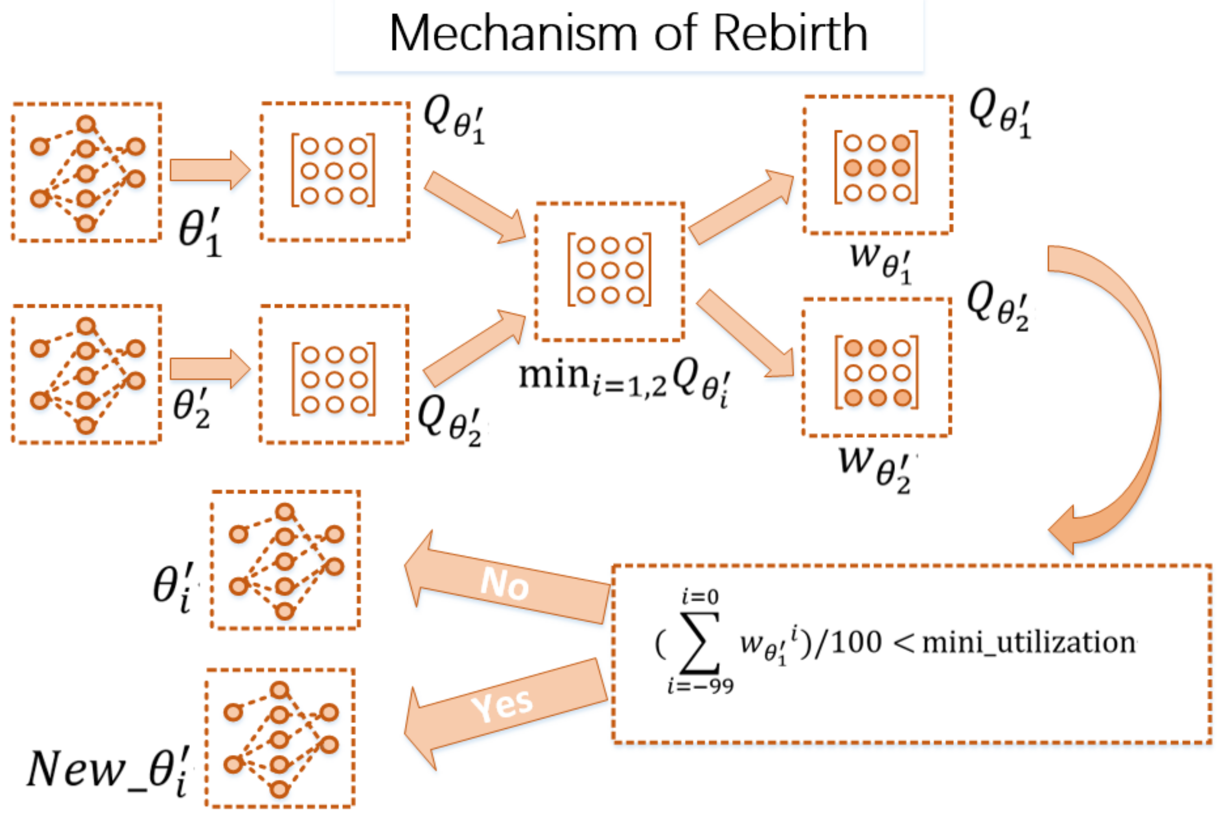
In order to build a better target critic network, this paper designs and establishes an target critic network elimination and rebirth mechanism to suppress overestimation bias of Q value. This mechanism is based on the ability to eliminate poor target critic networks when the elimination conditions are met, and rebuild a new set of network nodes to continue to be used for the evaluation mechanism of actor networks. 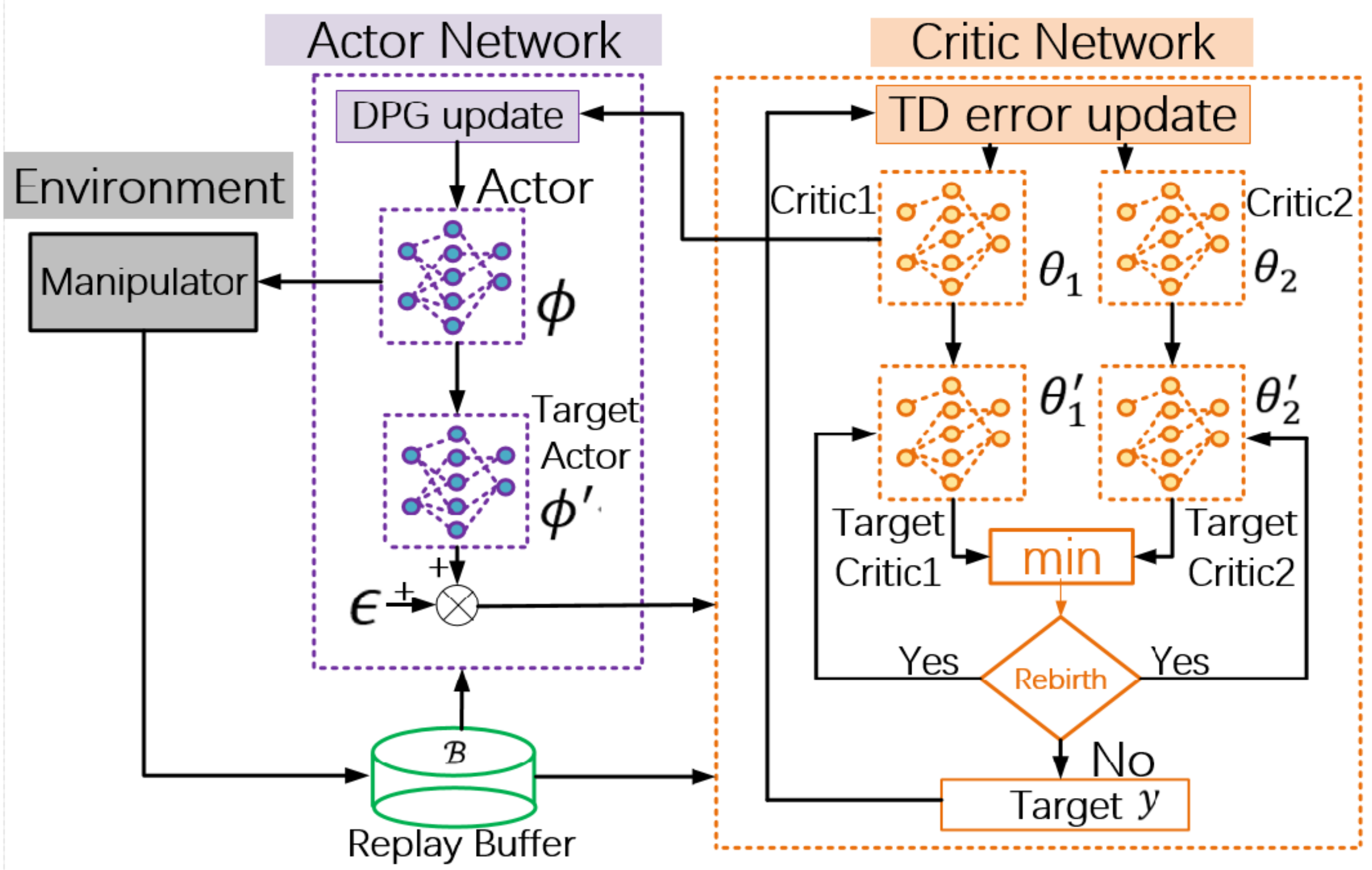Figure 3 shows the RTD3 network structure and shows RTD3 pseudocode through Algorithm 1, where the Rebirth Target Networks section is detailed by pseudocode in the Figure 4 Mechanism of Rebirth and Algorithm 2 Rebirth Target Networks.

In practice, RTD3 network structure diagram uses selecting the source of smaller Q value and evaluating the proportion of network as the condition to rebuild the target critic network. By calculating the utilization percentage of the first 100 Q-values selected for the network, the goal target critic network which is less than the minimum utillization rate $W_{\min }$ will be rebuilt. In order to ensure that the goal target critic network after rebirth has time for learning and adapting, the goal target critic network after rebirth will be protected for a certain time. During the protection time, the rebirth goal target critic network no longer accepts the rebirth mechanism operation.

$$\overline{w_{{\theta }_1^{\prime }}}==\left(\sum _{i=-99}^{i=0}{w}_{{\theta }_1^{\prime }}^i\right)/100,$$

(16)

$$\overline{w_{{\theta }_2^{\prime }}}==\left(\sum _{i=-99}^{i=0}{w}_{{\theta }_2^{\prime }}^i\right)/100,$$

(17)

where $w_{{\theta }_1^{\prime }}^i,w_{{\theta }_2^{\prime }}^i$ means totally 100 Q values using percentage, form $i=0$ at the current training moment to $i=-99$ at the current 99 training moments. $w_{{\theta }_1^{\prime }},w_{{\theta }_2^{\prime }}$ represent the average utilization percentage of the Q values given by the two Target Cirtic Networks at the current time $i=0$, respectively.

Algorithm 1 Algorithm RTD3.

1: Initialize critic networks $Q_{{\theta }_1},Q_{{\theta }_2}$ and actor network ${\pi }_{\varphi }$ with random parameters ${\theta }_1,{\theta }_2,\varphi$; 2: Initialize target networks $Q_{{\theta }_1^{\prime }},Q_{{\theta }_2^{\prime }},{\pi }_{{\varphi }^{\prime }}$; 3: Target network node assignment ${\theta }_1\to {\theta }_1^{\prime },{\theta }_2\to {\theta }_2^{\prime },\varphi \to {\varphi }^{\prime }$; 4: Initialize replay buffer $\mathcal{B}$; 5: for t = 1 to T do 6:   Select action with exploration noise $a\sim {\pi }_{\varphi }+ϵ,ϵ\sim N(0,\sigma )$; 7:   Store transition tuple (s, a, r, s’) in $\mathcal{B}$; 8:   if${ Sum}_{\mathcal{B}}<mini\_batch$then 9:     Return; 10:   end if 11:   Sample mini-batch of N transition (s, a, r, s’) from $\mathcal{B}$; $$\begin{array}{c}\tilde{a}\leftarrow {\pi }_{{\varphi }^{\prime }}\left(s^{\prime }\right)+ϵ,ϵ\sim clip(N(0,\tilde{\sigma }),-c,c);\hfill \\ y=r+\gamma {min}_{i=1,2}{Q}_{{\theta }_i^{\prime }}(s^{\prime },\tilde{a});\hfill \end{array}$$ 12:   Statistical calculation of Q value utilization ratio $w_{{\theta }_1^{\prime }},w_{{\theta }_2^{\prime }}$; 13:   if$\overline{w_{{\theta }_1^{\prime }}}<mini\_utilization$then 14:     Rebirth target networks ${\theta }_1^{\prime }$; 15:   end if 16:   if$\overline{w_{{\theta }_2^{\prime }}}<mini\_utilization$then 17:     Rebirth target networks ${\theta }_2^{\prime }$; 18:   end if 19:   Update critics ${\theta }_i\leftarrow {argmin}_{{\theta }_i}{N}^{-1}\sum {(y-Q_{{\theta }_i}(s,a))}^2$; 20:   if$tmodd$then 21:     Update $\varphi$ by the deterministic policy gradient: $$\begin{array}{c}\hfill {▽}_{\varphi }J\left(\varphi \right)=N^{-1}\sum {▽}_a{Q}_{{\theta }_1(s,a)}{|}_{a={\pi }_{\varphi }\left(s\right)}{▽}_{\varphi }{\pi }_{\varphi }\left(s\right);\end{array}$$ 22:     Update target networks: $$\begin{array}{c}\hfill {\theta }_i^{\prime }\leftarrow \tau {\theta }_i+(1-\tau ){\theta }_i^{\prime },\varphi \leftarrow \tau \varphi +(1-\tau ){\varphi }^{\prime };\end{array}$$ 23:   end if 24: end for

Through the rebirth mechanism of target critic network in Figure 4, the network that is not suitable for evaluating the learning of the manipulator can be eliminated in time continuously. The target critic network that is rebuilt can participate in the process of evaluating the learning of the manipulator.

With this scheme design, the number of target critic networks can be reduced and the requirement of computer computing ability in training process can be reduced.

Algorithm 2 Algorithm Rebirth Target Networks.

1: Initialize mini_utilization $W_{min}$ and Protection time $T_p$; 2: if Protection time $T_p>0$ then 3:   Return; 4: end if 5: Statistical calculation $\overline{w_{{\theta }_1^{\prime }}},\overline{w_{{\theta }_2^{\prime }}}$; 6: if$\overline{w_{{\theta }_1^{\prime }}}<W_{min}$then 7:   Rebirth target critic network ${\theta }_1^{\prime }$ with random parameter; 8:   Reset Protection time $T_p$; 9:   Return; 10: end if 11: if$\overline{w_{{\theta }_2^{\prime }}}<W_{min}$then 12:   Rebirth target critic network ${\theta }_2^{\prime }$ with random parameter; 13:   Reset Protection time $T_p$; 14:   Return; 15: end if 16: Update protection time $T_p\leftarrow T_p-1$.

5. Efficient Distance

In the framework of DRL, different network structures can be evaluated by setting the same reward function to give feedback on reward scores. However, there are obvious inappropriateness of this criterion for multi-DOF manipulators. For this article, through the design of a variety of reward functions, there itself exists the use of different dimensions of information, so the reward score can not fairly evaluate the effect of different forms of reward functions. Therefore, using the DRL framework to learn the motion ability of a multi-DOF manipulator requires a specially defined performance evaluation index for the multi-DOF manipulator’s motion ability.

The evaluation index designed in this paper is the efficiency distance, which is used as the evaluation index to evaluate the kinematic learning ability of the multi-DOF manipulator. This index can make a fairer comparison between the improved reward function and the learning effect of the multi-DOF manipulator’s motion ability with the DRL framework.

Efficient distance $D_e$ is defined as:

$$D_e=\frac{{\sum }_{i=1}^{N_{step\_time}}(L_{Init}-D_i)}{L_{Init}{N}_{step\_time}}.$$

(18)

The parameters in Equation (18) are explained as follows.

$L_{Init}$: Euclidean distance from initial position to generated random position;

$D_i$: Euclidean distance from the end of the real-time manipulator to the randomly generated position for the times movement in the same;

$N_{step\_time}$: Total number of decision-making times for the actual motion of a manipulator in the same.

6. Experiments and Discussions

The software and hardware configuration of this experiment is shown in

Table 2. Software and hardware configuration.

Hardware Configuration
CPU	AMD Ryzen 7 3750 H with Radeon Vega Mobile Gfx 2.30 GHz
Vision	Windows 10 64 bit
RAM	8 GB
Software Configuration
Pycharm	Community Edition 2019.3.3
Torch	1.5.0 + cpu
Torchaudio	0.7.0
Torchvision	0.6.0 + cpu

, and the configuration of network parameters is shown in

Table 3. Network parameter settings.

Parameter	Value
Actor learning rate	0.001
Critic learning rate	0.001
Target actor learning rate	0.001
Target critic learning rate	0.001
Input dims	6
DNN size	$64\times 64\times 128$
Output dims	3
Batch size	100
Optimizer	adam
Update delay	10

.

The fewer the number of network nodes, the fewer the number of network layers and the smaller the batch size, the less computational power was needed in the training process. Therefore, the following parameters were selected in this experiment. The learning rate of actor network and critical network was 0.001 according to experience. This also showed that RTD3 algorithm could use a small network to show strong expression ability.

Universal Robots introduced the first collaborative robot in 2009, UR5, with a weight of 18 kg, a load of up to 5 kg and a working radius of 85 cm. The UR5 manipulator model was used in this experiment. The kinematics model of UR5 was established by D-H parameters method, which was used as the observation method to sense the workspace position of the manipulator end-effector. In

Table 4. The D-H parameters of UR5.

Joint	a	d	$\mathit{\alpha }$	$\mathit{\theta }$
1	0	0.0892	$\pi /2$	${\theta }_1$
2	−0.4250	0	0	${\theta }_2$
3	−0.3923	0	0	${\theta }_3$
4	0	0.1092	$\pi /2$	${\theta }_4$
5	0	0.0946	$-\pi /$2	${\theta }_5$
6	0	0.0823	0	${\theta }_6$

, we show the DH parameters of UR, where a is the length of the link, d is the offset of the link, $\alpha$ is the twist angle of the link, $\theta$ is the joint angle. The units of a and d are meters, and the units of $\alpha$ and $\theta$ are radians.

By defining the link coordinate system and corresponding link parameters of UR5, the kinematic equation of UR5 could be directly established. The homogeneous transformation matrix of each link could be calculated by the value of the link parameter of UR5 as Equation (19).

$${}_i^{i-1}T=\left(\begin{array}{cccc}cos\left({\theta }_i\right)& -sin\left({\theta }_i\right)cos\left({\theta }_i\right)& sin\left({\theta }_i\right)sin\left({\alpha }_i\right)& a_{i}cos\left({\theta }_i\right)\\ sin\left({\theta }_i\right)& cos\left({\theta }_i\right)cos\left({\alpha }_i\right)& -cos\left({\theta }_i\right)sin\left({\alpha }_i\right)& a_{i}sin\left({\theta }_i\right)\\ 0& sin\left({\alpha }_i\right)& cos\left({\alpha }_i\right)& d_i\\ 0& 0& 0& 1\end{array}\right)$$

(19)

By multiplying these homogeneous transformation matrices, the homogeneous transformation matrix of the coordinate system $\left\{E\right\}$ of the end-effector of the manipulator relative to the base coordinate system $\left\{B\right\}$ of the manipulator could be obtained, which was given as:

$${}_6^{0}T={}_1^{0}T{}_2^{1}T{}_3^{2}T{}_4^{3}T{}_5^{4}T{}_6^{5}T$$

(20)

Homogeneous transformation matrix T is a function of six joint variables. With this function, the position of the end-effector of the manipulator in the Cartesian coordinate system could be calculated.

In the model, the position information of the end-effector of the manipulator was obtained by the forward kinematics solution based on the angle of each joint of the manipulator. In the workspace of UR5 manipulator, with the same initial position, the end-effector of the manipulator generates the target position randomly during the 60,000 episodes of training to train the DRL network. In the experiment, $Join{t}_4$, $Join{t}_5$ and $Join{t}_6$ were determined to keep locked state, and the 6DOF manipulator was changed into 3DOF manipulator for deep reinforcement learning. The position deviation $dx$, $dy$ and $dz$ between the end-effector of the manipulator and the target position were taken as the input of the deep reinforcement learning network, and the joint angle increments $d{\theta }_{Joint1}$, $d{\theta }_{Joint2}$ and $d{\theta }_{Joint3}$ were taken as the output.

6.1. Effect of Step-by-Step Reward Function

In order to verify the effect of the step-by-step reward function, a comparative experiment was conducted between the step-by-step reward function, distance reward and azimuth reward function. The TD3 network was used to carry out the experiment with four groups of randomly initialized network node parameters. Under the same network environment configuration, 60,000 random target locations were generated in the workspace of the 3DOF manipulator to verify the effect of the step-by-step reward function. The step-by-step reward function has been mentioned before, and the composition of the distance reward function is Equation (21). This reward value adopts negative reward function, negatively correlated with distance.

$$R_{distance\_reward}=-{\lambda }_3\left|\overrightarrow{ST}\right|,$$

(21)

where ${\lambda }_3$ is a positive constant. In the coordinate system of the base of the manipulator, the azimuth reward function was formed by comparing the angle and distance of the current position with the target position. The azimuth reward function was given as:

$$R_{azimuth\_reward}={\lambda }_4{\phi }_3-{\lambda }_5\left|\overrightarrow{ST}\right|$$

(22)

where ${\phi }_3=\frac{\overrightarrow{OT}·\overrightarrow{OS}}{|\overrightarrow{OT}|·|\overrightarrow{OS}|}$, ${\lambda }_5$ is a positive constant. In different angle intervals, ${\lambda }_4$ had a different constant.

In this paper, the above three reward functions were combined into reward function(1) to reward function(4) by combination form as

Table 5. Four reward functions.

	Distance Reward	Step-by-Step Reward Function	Azimuth Reward
reward function(1)		✓
reward function(2)	✓
reward function(3)			✓
reward function(4)		✓	✓

. The improvement effect was proved by comparative experiments.

Four lots of random initialization of network node parameters were used for comparative experiments, namely Network(1) to Network(4). The effectiveness of the improved algorithm was proved by several experiments of random initialization of network node parameters. It should be noted that Network(1) to Network(4) in different comparative tests had different initialization network node parameters.

The comparison experiment shows that the step-by-step reward function had a better efficient distance than the distance reward function in

Table 6. The efficient distances of reward function(1) and reward function(2) for four times of randomly initialized network node parameters.

Reward Function Category	Network(1)	Nework(2)	Network(3)	Network(4)
Reward function(1)	91.76 %	91.08%	88.98%	84.88%
Reward function(2)	85.01 %	76.04%	75.54%	77.59%

and Figure 5. The average efficient distance obtained by the four-time random initialization of the step-by-step reward function was 89.18%, while the distance reward function just had an average efficient distance of 78.66%. In the TD3 network structure, the step-by-step reward function could improve the motion ability of the 3DOF manipulator by 10.63% compared with the distance reward function.

The comparison experiment shows that the composite reward function with the step-by-step reward function had a better efficient distance than the azimuth reward function in

Table 7. The efficient distances of reward function(3) and reward function(4) for four times of randomly initialized network node parameters.

Reward Function Category	Network(1)	Network(2)	Network(3)	Network(4)
Reward function(3)	58.23%	79.31%	75.35%	−165.02%
Reward function(4)	91.71%	91.14%	90.44%	91.26%

and Figure 6. The average efficient distance obtained with the four-time random initialization of the composite function (step-by-step reward function + azimuth reward function) was 91.14%, while the corresponding average efficient distance of the azimuth reward function was 11.97%. Excluding the Network(4) data of network divergence, the average efficient distance of the composite function (step reward function + azimuth reward function) was 91.10%, and that of the azimuth reward function was 70.96%. In the TD3 network structure, a step-by-step reward function was added to improve the motion ability of the 3DOF manipulator by 20.13%.

6.2. Comparison of Experimental Effects between RTD3 and TD3

This part of the experiment compared the difference in learning ability between TD3 and RTD3 which further suppressed the overestimated bias of Q value. The experiment was carried out with through four random initialization of network node parameters. Under the settings of four reward functions, the network training was conducted with the use of 60,000 random generated target locations.

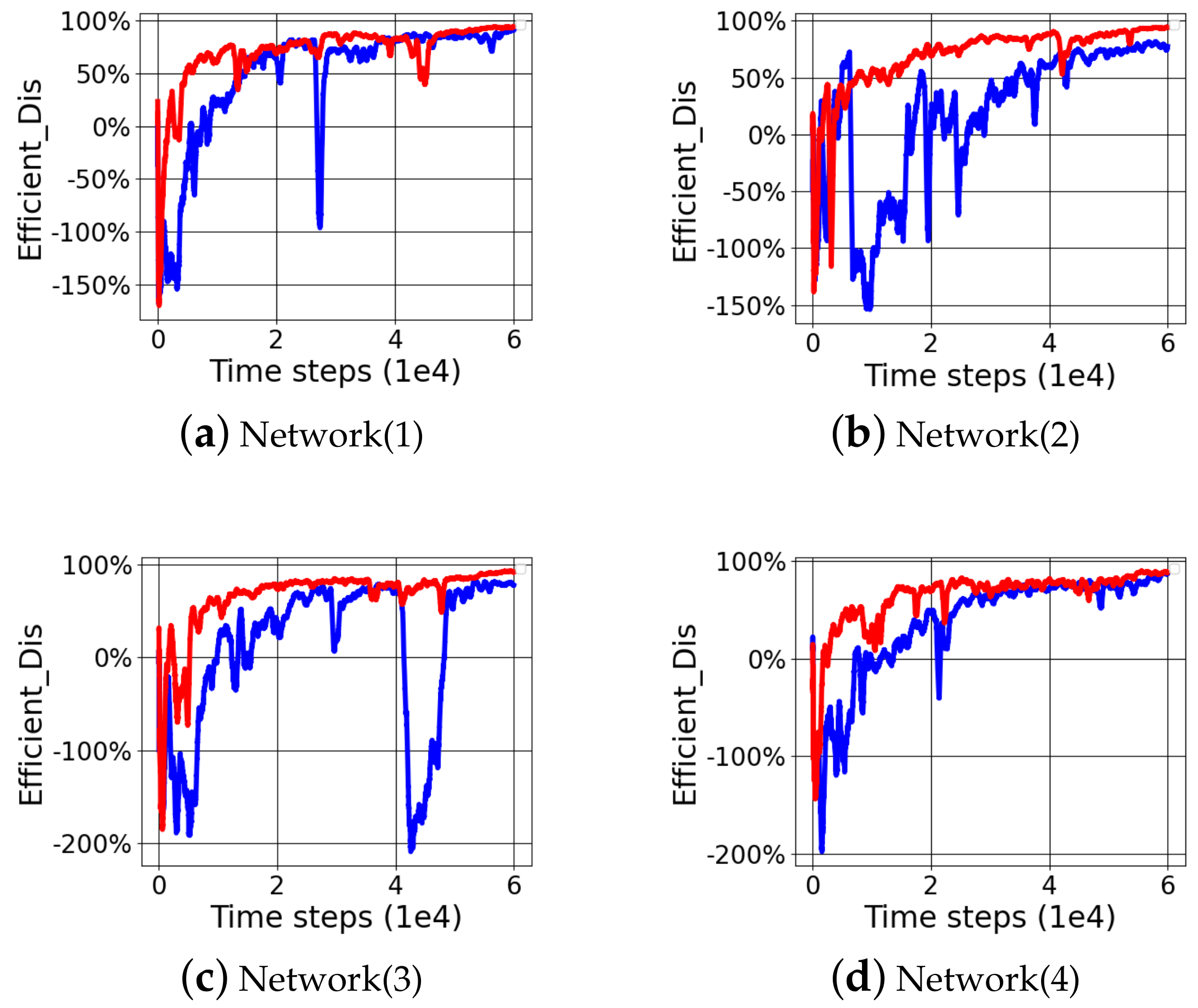
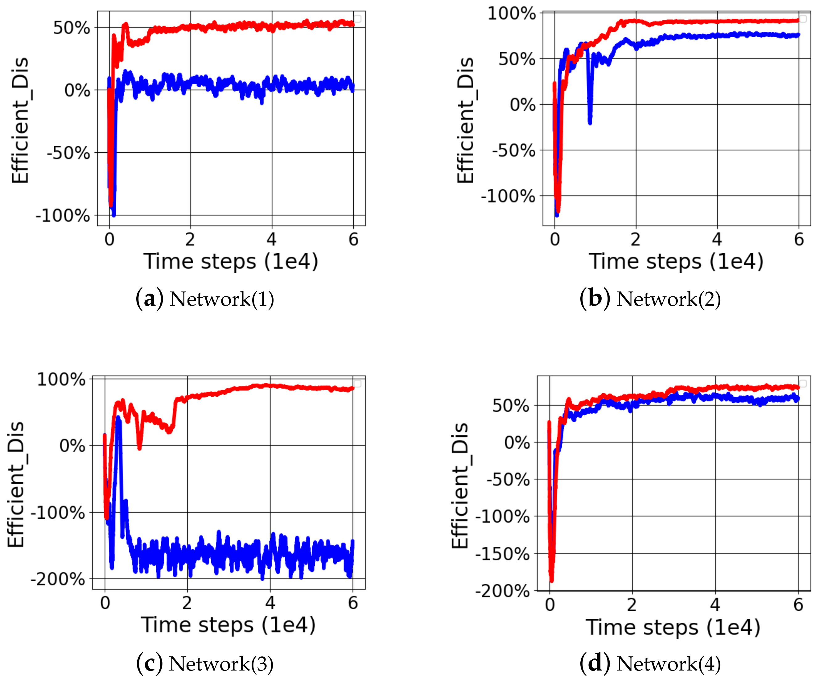
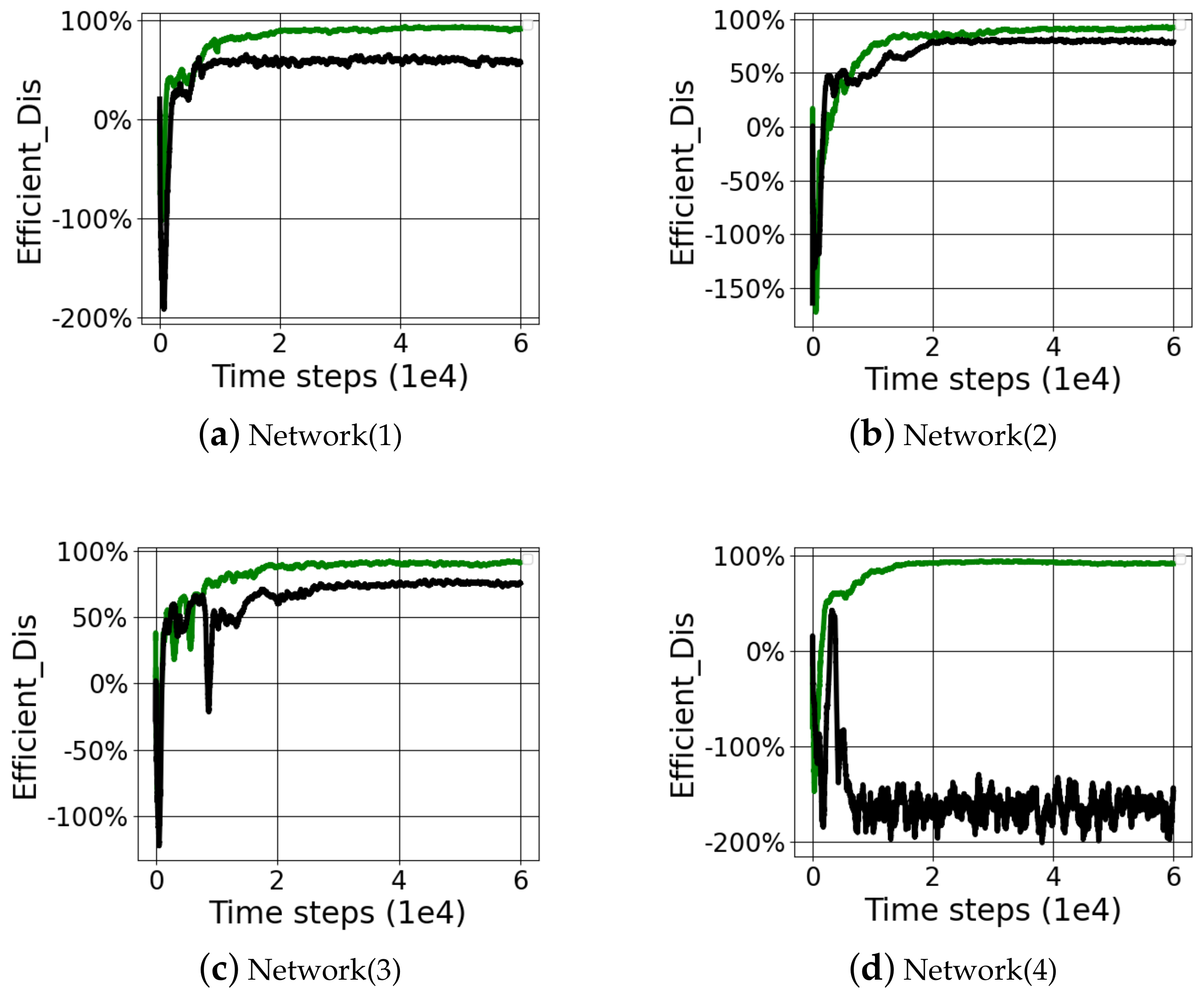
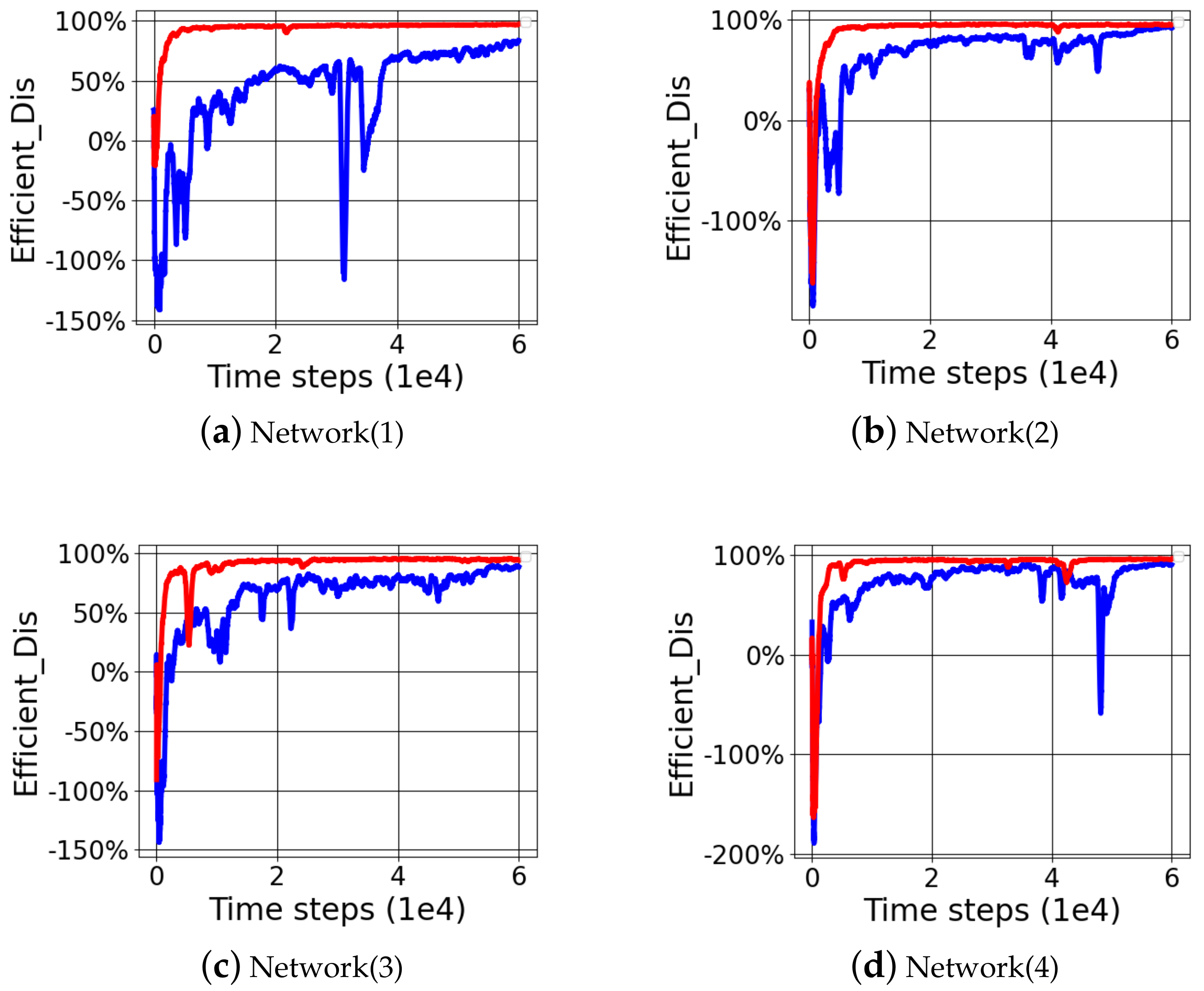
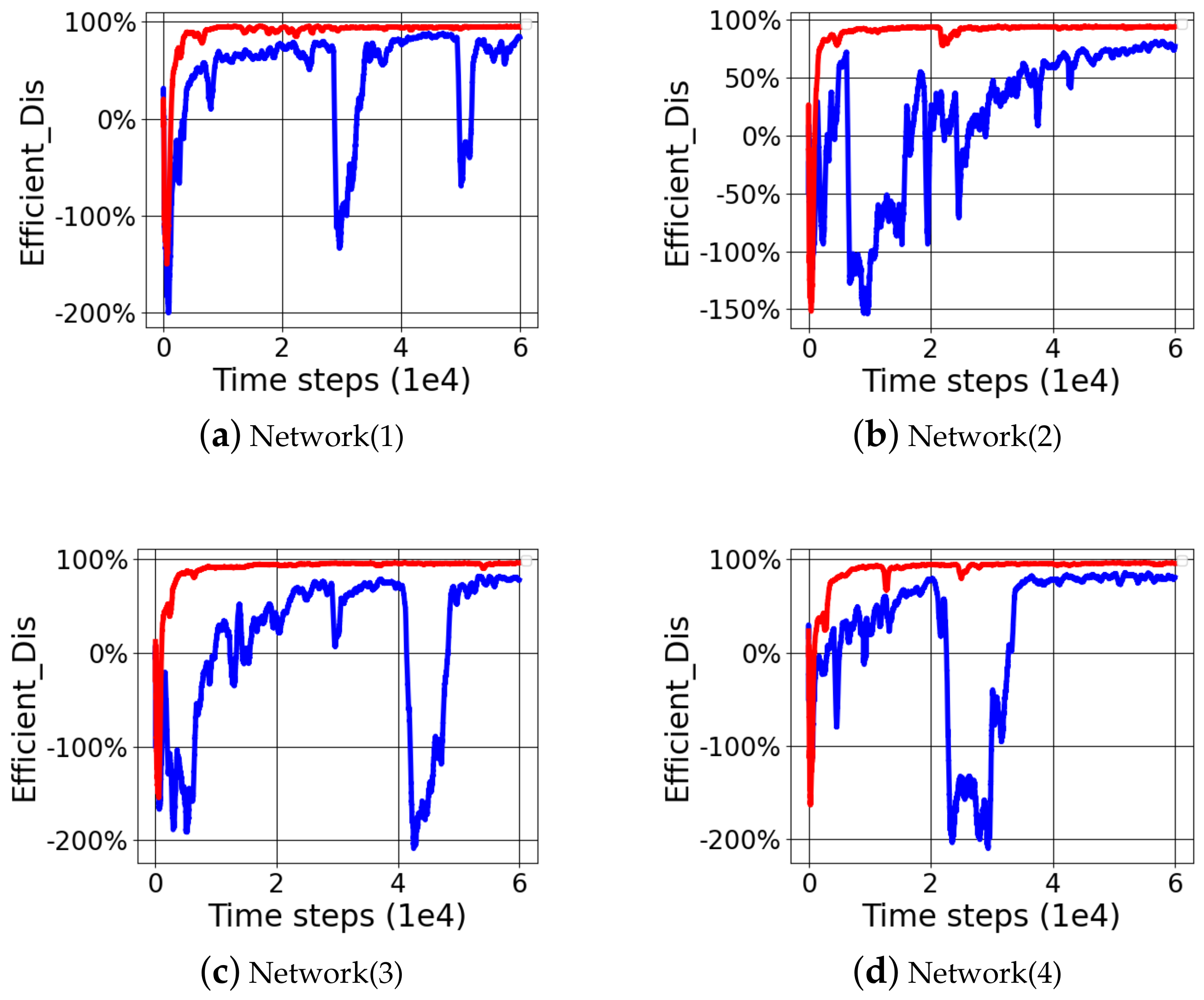
The results of four random network generations for RTD3 and TD3 networks under the same initial network conditions showed that the improved RTD3 network structure could achieve better learning results. Through Figure 7, under the condition of reward function(1), RTD3 achieves higher efficient distance and more stable convergence compared with TD3. Especially for the reward function(2) and reward function(3), which could not help the manipulator to learn better by setting appropriate reward function, the improved RTD3 could significantly improve the efficient distance. 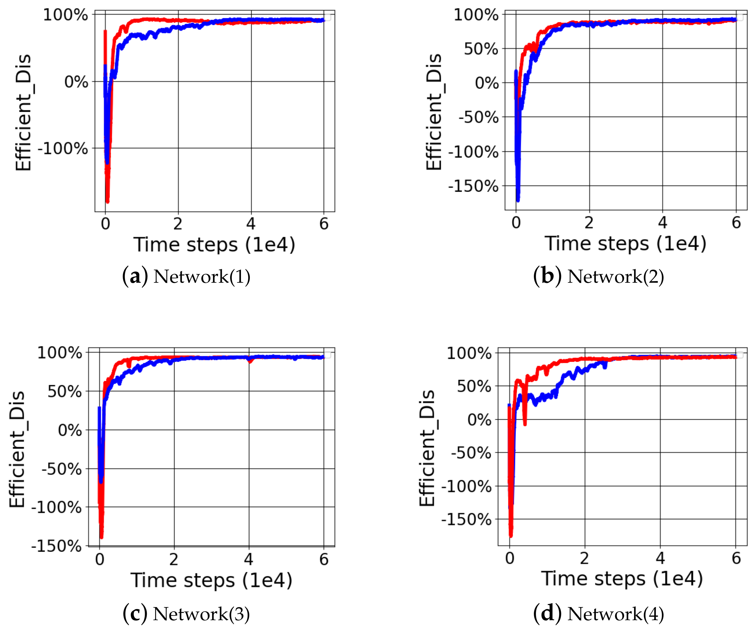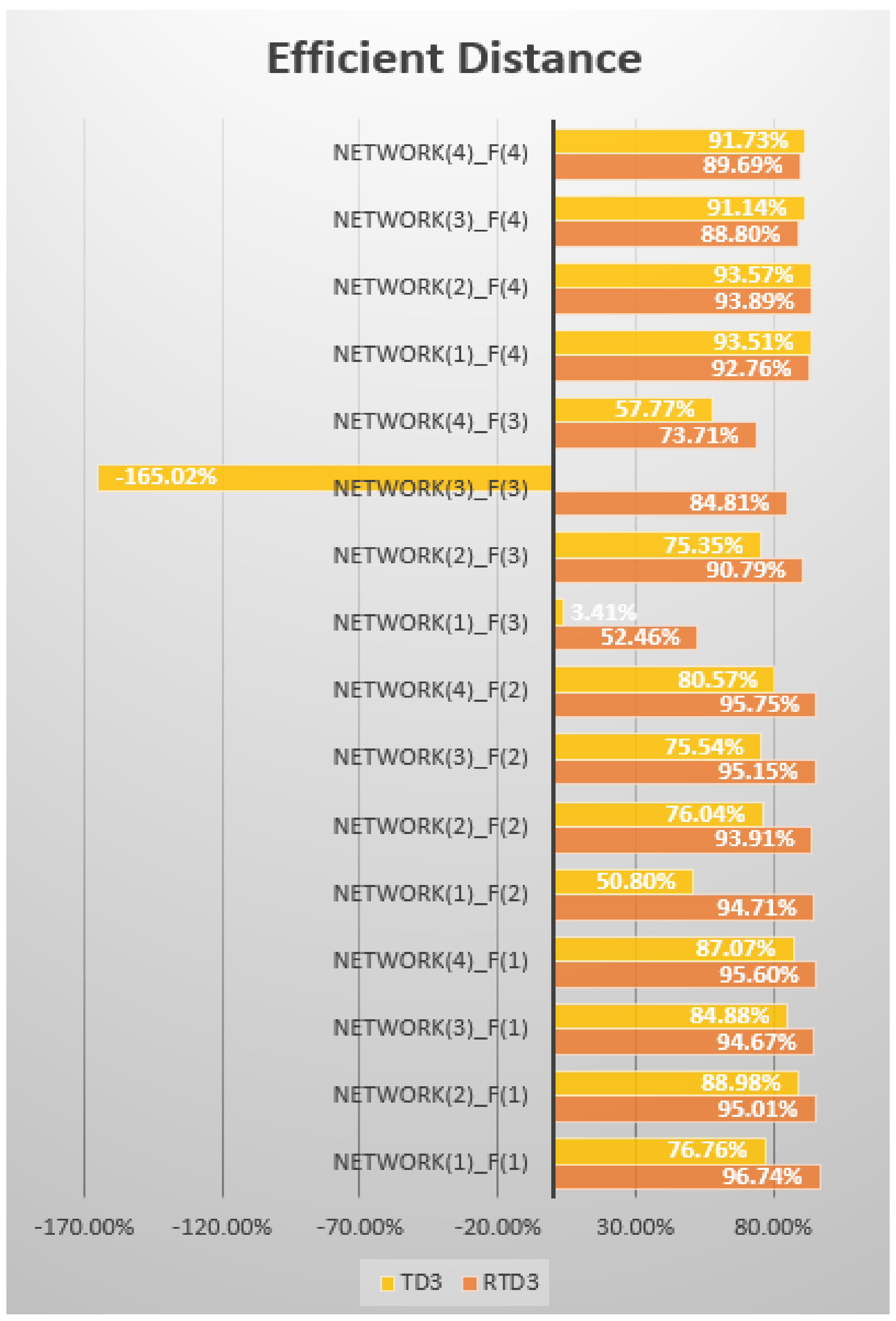Especially when the initial network node parameters could not learn better, such as reward function(3), randomly generated Network(1) and Network(3), the improved RTD3 could greatly improve the learning effect in Figure 8 and Figure 9. The average efficient distance of RTD3 was 89.28%, which was higher than 60.13% of TD3. RTD3 improved learning efficiency by 29.15%. When wiping out the controversial Network(3)_F(3) comparative experiment data, the average efficient distance index of RTD3 was 89.58%, which was higher than 75.14% of TD3. RTD3 improved learning efficiency by 14.44%. Although both RTD3 and TD3 can get same results under the condition of well-designed reward function, RTD3 is better than TD3 in convergence speed in Figure 10. We can compare all the experiments and see the comparison results intuitively through

Table 8. Under the four reward function settings, the average efficient distance of RTD3 and TD3 for four times of randomly initialized network node parameters when episode is in the range of 50,000 to 60,000.

Network Structure and Reward Function Categories	Network(1)	Network(2)	Network(3)	Network(4)
RTD3(1)	96.74%	95.01%	94.67%	95.60%
TD3(1)	76.76%	88.98%	84.88%	87.07%
RTD3(2)	94.71%	93.91%	95.15%	95.75%
TD3(2)	50.80%	50.80%	75.54%	80.57%
RTD3(3)	52.46%	90.79%	84.81%	73.71%
TD3(3)	3.41%	75.35%	−165.02%	57.77%
RTD3(4)	92.76%	93.89%	88.80%	89.69%
TD3(4)	93.51%	93.57%	91.14%	91.73%

and Figure 11.

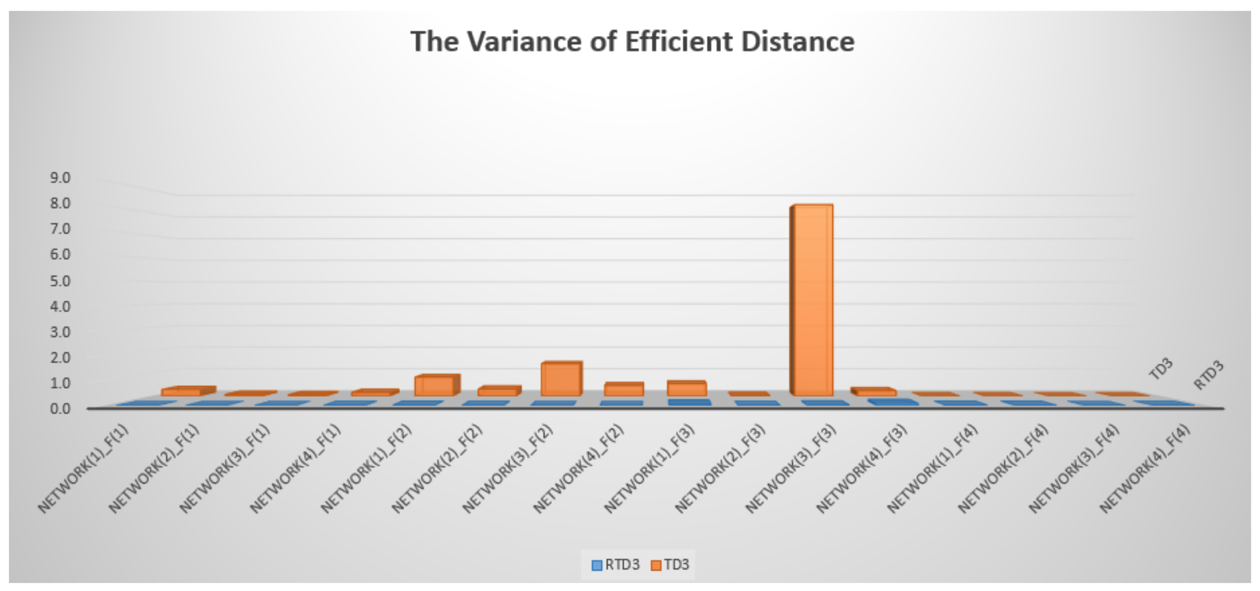
Through the comparison of learning process, we can see that the improved RTD3 network structure could achieve a more robust learning process than the TD3 network structure, and there was no severe network oscillation in the overall process. By comparing the variances of efficient distances when episode ranged from 30,000 to 60,000, the differences in learning robustness of network structures could be characterized.

By comparing the variances, we can see that RTD3 was better in learning ability and better in robustness in learning process in

Table 9. Under four reward function settings, the variances of efficient distances of RTD3 and TD3 for four times of randomly initialized network node parameters when episode varies from 30,000 to 60,000.

Network Structure and Reward Function Categories	Network(1)	Network(2)	Network(3)	Network(4)
RTD3(1)	0.001159	0.003495	0.002349	0.007059
TD3(1)	0.291893	0.075529	0.060792	0.162559
RTD3(2)	0.015039	0.006725	0.003478	0.001854
TD3(2)	0.823852	0.308610	1.408862	0.463721
RTD3(3)	0.071677	0.006649	0.026182	0.090065
TD3(3)	0.542213	0.032461	8.347054	0.238845
RTD3(4)	0.016182	0.012684	0.002566	0.006161
TD3(4)	0.008251	0.008009	0.003014	0.005266

and Figure 12. Compared with the TD3 network structure, the average efficient distance variance of RTD3 was 0.0171, while that of TD3 was 0.7988, which was 46.71 times that of RTD3. When wiping out the controversial Network(3)_F(3) comparative experimental data, the average efficient distance variance of RTD3 was 0.0165, that of TD3 was 0.2956, which was 17.94 times that of RTD3. In some comparative experiments, the variance of efficient distance of RTD3 was even hundreds of times better than that of TD3. It also showed that RTD3 network structure could show better stability in the middle and late learning stages of multi-DOF manipulator learning.

7. Conclusions

Through a series of comparative experiments, the step-by-step reward function proposed in this paper can better reflect the learning characteristics of the multi-DOF manipulator, and the deep reinforcement learning method can make the multi-DOF manipulator obtain better motion ability. The RTD3 algorithm proposed in this paper achieves higher learning efficiency and mobility than the TD3 algorithm in the experimental environment of multi-DOF manipulators. Especially when the parameters of randomly initialized network nodes are not good, TD3 can not show a good effect of exploring and attempting training, while RTD3 can still obtain a better promotion of the learning efficiency and mobility of multi-DOF manipulators. Through all of the above experiments, it is verified and illustrated that the two improvements proposed in this paper have achieved the expected results in improving and helping the learning of the motion ability of the multi-DOF manipulator. The two improvements are in conformity with the motion characteristics and rules of the multi-DOF manipulator.

Through the research work of this paper, our team found that RTD3 algorithm can use smaller models to complete some learning tasks that can only be completed by larger models. Compared with the large model of deep learning, RTD3 algorithm can use the smaller model on the premise of effective learning. RTD3 algorithm effectively improves the perception ability of small model.

Through the analysis of the experimental results, RTD3 algorithm can continuously detect the proportion of Q value predicted by two target critical networks in the early training period. RTD3 algorithm can regenerate the target critical network which always produces high overestimation bias of Q values in a certain period of time by further analysis and setting the occupancy ratio threshold. This paper also finds that the method of restraining the overestimation bias of Q value has a significant improvement effect on the deterministic policy gradient method. It is found that the threshold of occupancy ratio is sensitive to the learning ability of the deterministic policy gradient method. This can be used as a direction for further research in the future.

Aiming at the motion ability of static manipulator, it is mostly open-loop control in the current application of real life and production activities, that is, firstly, the kinematics model of the manipulator is established, then the target position is detected by sensors, and then the kinematics inverse solution of the target position is carried out in the kinematics model of the manipulator, and finally the trajectory of the manipulator is obtained through the planning algorithm similar to spline interpolation to reach target position. In this paper, we no longer look for a network structure to represent the kinematics model of the manipulator through intelligent algorithm training, that is, we no longer regard the manipulator end-effector reaching the target position as a process of motion path. In this paper, the current state of the manipulator (the angle of each joints of the manipulator) and the position deviation between the end-effector and the target position of the manipulator are taken as the input information to maximize the use of the cooperation between human arm and human eyes. Through bionics, the RTD3 algorithm is further used to represent a more advanced level of intelligence. In this aspect, in the future, a camera will be placed at the end of the manipulator to imitate human eyes, so as to realize the cooperation between the arm and the eyes in a more biological sense.

Of course, there are still many aspects worthy of study and promotion in the current research work. Compared with the mature control method based on manipulator motion model, the current RTD3 algorithm can not be applied in practical application, and its performance needs to be improved. In the future, we need to achieve more in-depth research on the high-precision capture task of dynamic target.