Trajectory Planning Algorithm of UAV Based on System Positioning Accuracy Constraints

Abstract

This paper describes a novel trajectory planning algorithm for an unmanned aerial vehicle (UAV) under the constraints of system positioning accuracy. Due to the limitation of the system structure, a UAV cannot accurately locate itself. Once the positioning error accumulates to a certain degree, the mission may fail. This method focuses on correcting the error during the flight process of a UAV. The improved genetic algorithm (GA) and A* algorithm are used in trajectory planning to ensure the UAV has the shortest trajectory length from the starting point to the ending point under multiple constraints and the least number of error corrections.

1. Introduction

An unmanned aerial vehicle (UAV) is an aircraft capable of completing missions with the autonomous flight capability. UAVs are currently widely used in vision systems, such as cargo transfer [1], object detection [2,3,4], and vision-assisted navigation [5,6,7].

The idea for scientists to develop UAVs is to fly autonomously and accomplish specific tasks. In modern warfare, the air defense system is constantly improving, and air defense technology is becoming more and more advanced. Thus, improving the autonomy of unmanned aerial vehicles is an important trend for the future. Trajectory planning is a key technology to improve the autonomy of a UAV and an effective means to implement flight missions. It has important significance in both theoretical and practical applications. The aircraft path planning can effectively ensure the operational performance of a UAV, which provides technical support for a UAV to successfully complete the flight mission, realize the autonomous control of a UAV, and to complete the autonomous flight.

Trajectory planning refers to the planning of an optimal flight path of the aircraft between the starting point and the ending point, considering factors such as fuel consumption, maneuverability, arrival time, flight area, and threat level. Trajectory planning is an important guarantee for the successful completion of a UAV and one of the key technologies for mission planning systems.

Due to technical limitations, in the early 1980s, trajectory planning relied heavily on manual operations by technicians. With the continuous development and improvement of the prevention and control system and technology, the accuracy requirements of a UAV for planning the trajectory are getting higher and higher, and artificial path planning has become more and more difficult to meet the requirements. With the rapid development of communication technology, various methods for detecting flight environment information have emerged endlessly, which makes the information obtained by the trajectory planners more and more abundant. In order to improve flight accuracy, the planned trajectory should satisfy the requirements of terrain following, terrain avoidance, and threat avoidance while satisfying the performance constraints of the aircraft. Due to the complexity and variety of these constraints, it is difficult to handle and complete such complex tasks in manually.

In order to realize the autonomous trajectory planning under different planning environments, scientists have carried out in-depth research on the trajectory planning of an UAV, and proposed various algorithms, such as the Voronoi diagram method [8,9,10,11], A* algorithm [12,13,14], particle swarm optimization (PSO) algorithm [15,16,17], genetic algorithm [18,19,20], neural network algorithm [21,22], artificial potential field method [23,24,25], simulated annealing algorithm [26], and so on.

The process of finding the best trajectory includes consideration of constraints. The optimal path must produce an optimal objective function and satisfy multiple constraints. However, conventional methods can only handle one objective function at a time, and they cannot handle optimization problems involving two or more objective functions. Thus, a combined objective function is formed by mathematically aggregating two or more separate objective functions. The weighted values are introduced into the combined objective function formula to reflect its relative importance. In this work, we propose a trajectory path planning algorithm of a UAV based on genetic algorithm and A* algorithm under multiple constraints, and then satisfied the system positioning accuracy conditions.

The paper is organized as follows: Section 2 provides the necessary background: problem statement, model assumptions, and multiple constraints. Section 3 describes in detail an UAV trajectory planning Problem 1 based on positioning accuracy constraints, and uses an improved genetic algorithm to design a trajectory planning algorithm, and finally get the results of the trajectory planning. Section 4 describes in detail an UAV trajectory planning Problem 2 based on Problem 1, and uses an improved A* algorithm to design a trajectory planning algorithm, and finally get the results of the trajectory planning. Section 5 presents the performance comparison of the proposed algorithm with the traditional swarm intelligence algorithm. Section 6 concludes the paper and gives the further work.

2. Background

2.1. Problem Statement

In practical applications, the planning scope is often up to one million square kilometers, and the planning area environment is very complicated. In addition to the topographical factors, the planning process needs to consider various constraints such as aircraft maneuverability, penetration requirements, and flight missions. This research is a simplified version of the actual problem, without considering the aircraft’s maneuverability, penetration requirements, threats, and many other factors. However, there are multiple constraints.

In this research, we mainly consider the trajectory error correction problem of an UAV based on system positioning accuracy constraints. Due to system structure limitations, the positioning system of such aircraft cannot accurately locate itself. Once the positioning error accumulates to a certain extent, the task may fail. Therefore, correcting the positioning error during flight is an important task in UAV trajectory planning. The trajectory planning problem of an UAV is a complex multi-constrained optimization problem. UAV trajectory planning refers to considering the positioning error during the flight due to a series of factors such as the environment and weather during the flight. Therefore, some safe positions are assumed in the flight area (called correction points) for safety correction. In order to enable a UAV to follow the original trajectory planning from the starting point to the ending point, several correction points are needed in the flight area to correct the trajectory error of an UAV.

Under the premise of many constraints, the correct point is selected to correct the error of a UAV, and the best flight path from the starting point to the ending point is planned for an UAV, so that the number of times a UAV is corrected by the correct points during the flight is as small as possible, and the trajectory length is as small as possible. How to ensure that a UAV meets the various constraints and the optimal trajectory requirements, and to quickly and accurately obtain the true flight trajectory is the problem that needs to be solved urgently. In the aircraft trajectory planning problem, the standard planning problem is usually to establish a flight trajectory with the optimal cost function value through a pre-set cost function.

2.2. Model Assumptions and Multiple Constraints

The aim of this study is to find the best optimal trajectory planning for an UAV under the limit of the positional accuracy of a UAV system, which is a multi-constraint combinatorial optimization problem.

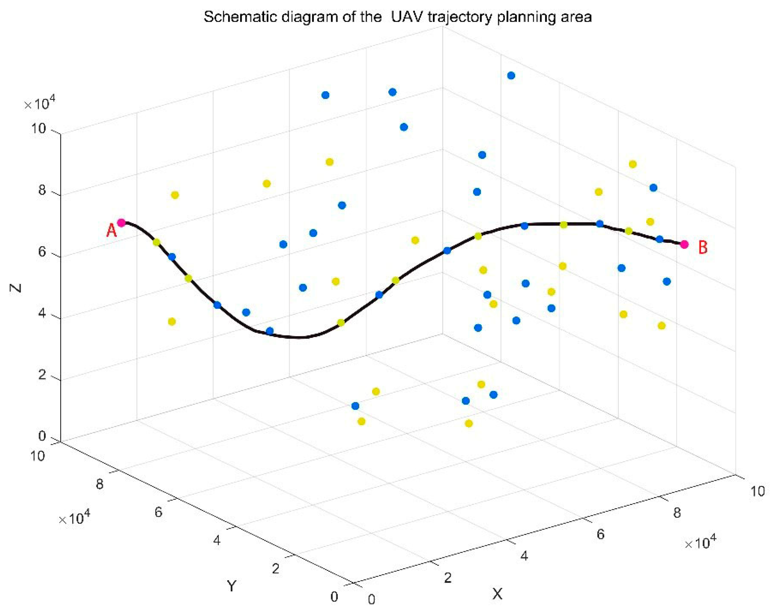
Assume that the flight area of an UAV and the safe positions is as shown in Figure 1. The starting point is A and the ending point is B. The constraints of its trajectory are as follows:

(1) A UAV needs real-time positioning during flight, and its positioning error includes vertical error and horizontal error. For every 1m flight, the vertical error and horizontal error will be increased by δ dedicated units, respectively. The vertical error and horizontal error should be less than θ units when reaching the ending point, and for the sake of simplification, assume that when the vertical error and the horizontal error are both less than θ units, an UAV can still follow as the planned trajectory to fly.

(2) A UAV needs to correct the positioning error during flight. There are some safety positions in the flight area (called correction points) can be used for error correction. The type of the correction point includes horizontal and vertical correction points. If a UAV reaches the correct point, the error can be corrected based on the type of the correct points, assuming that the safety positions in the flight area (i.e., the position of the correction points) is determined before flight trajectory planning. Figure 1 is a schematic diagram of a certain trajectory. If the vertical error and the horizontal error can be corrected in time, a UAV can fly according to the predetermined trajectory, and finally reaches the destination.

(3) At the starting point A, the vertical and horizontal error of an UAV are both zero.

(4) After the correction of the vertical error correction point, the vertical error will become zero and the horizontal error will remain unchanged.

(5) After the correction of the horizontal error correction point, the horizontal error will become zero and the vertical error will remain unchanged.

(6) Vertical error correction can be performed when the vertical error of the aircraft is not greater than ${\alpha }_1$units and the horizontal error is not greater than ${\alpha }_2$ units.

(7) Horizontal error correction can be performed when the vertical error of the aircraft is not greater than ${\beta }_1$units and the horizontal error is not greater than ${\beta }_2$units.

(8) An UAV is limited by the structure and control system during the turn and cannot complete the immediate turn (i.e., the direction of an UAV cannot be changed abruptly), if the minimum turning radius of an UAV is 200 m [27].

3. Problem 1

To plan a trajectory for an UAV from point A to point B, for the above-mentioned conditions (1) to (7), and comprehensively consider the following optimization goals: (A) the trajectory length is as small as possible; (B) the number of corrections through the correct points is as small as possible.

If the above-mentioned parameters of the data are:

${\alpha }_1$ = 25, ${\alpha }_2$ = 15, ${\beta }_1$ = 20, ${\beta }_2$ = 25, θ = 30, δ = 0.001.

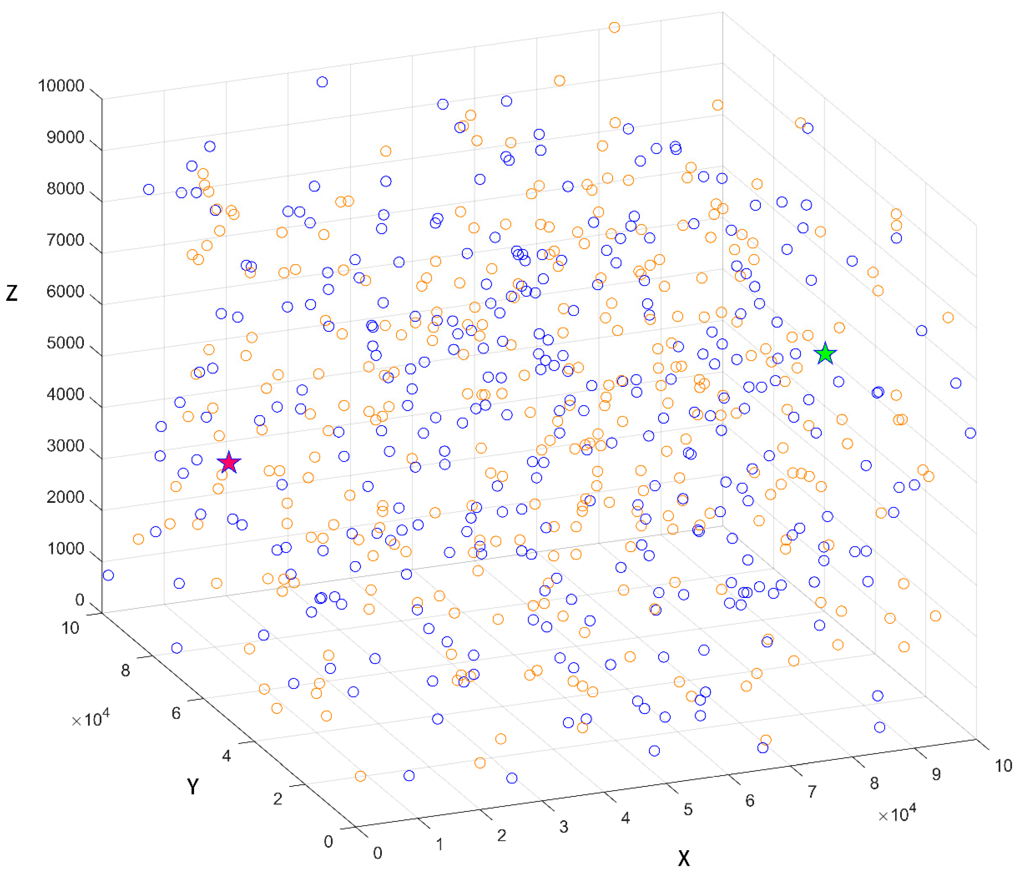
A data set contains the location and type of correction points.

Table 1. Some data of the data set [27].

The Number of the Correction Points	X-Coordinate	Y-Coordinate	Z-Coordinate	The Type of the Correction Points
0	0.00	50,000.00	5000.00	The Starting Point
1	33,070.83	2789.48	5163.52	0
2	54,832.89	49,179.22	1448.30	1
3	77,991.55	63,982.18	5945.82	0
4	16,937.18	84,714.34	5360.29	0
5	339.69	14,264.46	3857.85	1
6	3941.93	74,279.86	9702.92	1
7	45,474.01	26,849.48	6411.72	1
8	86,806.90	5351.31	4409.85	0
9	23,602.88	68,460.10	88.47	0
……	……	……	……	……
610	14,870.60	95,939.17	8248.84	0
611	93,009.57	4549.33	7882.61	1
612	100,000.00	59,652.34	5022.00	The Ending Point

shows some data of the data set. The unit of the coordinate is meter. There are 613 points in the data set. The number 0 is the starting point, the number 612 is the ending point, and the rest is correction points. The spatial position of each correction point is determined by the three-coordinate information of x, y, and z. For the type of the correction points, 0 represents the horizontal error correction point and 1 represents the vertical error correction point.

3.1. Multi-Constraints Optimization Problem

The focus of this research is to plan a trajectory for an UAV from the starting point to the ending point, and finding the optimal trajectory satisfied with the multi-constraints in Problem 1, so we build mathematical models of the problem.

3.1.1. Correction Area

The trajectory planned by a UAV is three-dimensional, and it is a space with many correction points. $\left(x,y,z\right)$is defined as the coordinates of correction point in the correction area, where x is the error in the horizontal direction, y is the error in the vertical direction, and z indicates the altitude. The physical space of the trajectory planning can be expressed as a set:

$$S=\left\{\left(x,y,z\right)\right|0\le x\le X_{\max },0\le y\le Y_{\max },0\le z\le Z_{\max }\}$$

(1)

where $X_{\max }$,$Y_{\max }$ and $Z_{\max }$ refer to the maximum values of the corresponding coordinates, which can be obtained from the data set. Moreover, from the data set, we can dram the vertical error correction point and the horizontal error correction point in three-dimensional space. Figure 2 is the result we have drawn with MATLAB.

3.1.2. Objective Function

Two objective optimization functions are proposed for minimizing the trajectory length of a UAV and the number of times an UAV has been corrected:

$$F_1=\min ({\displaystyle \sum }_{i=1}^m\left({\eta }_i+{\lambda }_i+h_i\right))$$

(2)

$$F_2=\min ({\displaystyle \sum }_{i=1}^m\left(a_i+b_i\right))$$

(3)

where F₁ represents the trajectory length of an UAV from the starting point A to the ending point B, F₂ represents the number of times an UAV has been corrected through the correction area, m represents the total number of corrections of an UAV throughout the flight, ${\eta }_i$ represents the distance of an UAV’s i-th flight, ${\lambda }_i$ represents the correction distance of the i-th flight to the vertical error correction point, $h_i$ represents the correction distance of the i-th flight to the horizontal error correction point, $a_i$ represents an UAV’s i-th flight reaches the vertical error correction point, and b_i represents a UAV’s i-th flight at the horizontal error correction point.

3.1.3. Multi-Constraints

The vertical and horizontal errors will increase by $\delta$ units when a UAV flies one meter each time. The vertical and horizontal errors should be less than $\theta$ units when the ending point is reached. Therefore, the total value of the vertical and horizontal errors of an UAV during the entire flight must be less than $\theta$, and the distance ${\eta }_i$ of each flight of a UAV will not exceed the displacement $l_{AB}$ of the entire trajectory:

$${\displaystyle \sum }_{i=1}^m{a}_i{\eta }_i\delta <\theta$$

(4)

$${\displaystyle \sum }_{i=1}^m{b}_i{\eta }_i\delta <\theta$$

(5)

$$0\le {\eta }_i\le l_{AB}$$

(6)

For the correction distance ${\lambda }_i$ meters of a UAV’s i-th flight to the vertical error correction point, when a UAV reaches the vertical error correction point, it is assumed that a UAV’s i-th flight,${\eta }_i$ meters will increase its vertical error by $\delta {\eta }_i$ units:

$${\lambda }_i=a_i{\eta }_i\delta ,i=1,\dots ,m$$

(7)

For the correction distance $h_i$meters of an UAV’s i-th flight to the vertical error correction point, when a UAV reaches the horizontal error correction point, it is assumed that a UAV’s i-th flight,${\eta }_i$ meters will increase its horizontal error by $\delta {\eta }_i$ units:

$$h_i=b_i{\eta }_i\delta ,i=1,\dots ,m$$

(8)

During the flight, a UAV is either corrected after reaching the vertical error correction point or reaching the horizontal error correction point. In order to perform error correction more accurately according to the type of error correction of the correction point, for the i-th flight, the binary variables $a_i$ and $b_i$ are introduced. The vertical error correction can be performed when a UAV’s vertical error is not greater than ${\alpha }_1$ units and the horizontal error is not greater than ${\alpha }_2$ units. The horizontal error correction can be performed when a UAV’s vertical error is not greater than ${\beta }_1$ units and the horizontal error is not greater than ${\beta }_2$ units. The binary variables $a_i$ and $b_i$ can be expressed as follows:

$$a_i=\{ \begin{array}{c}1, when UAV reaches the vertical error correction point,\\ 0, when UAV does not reach the vertical error correction point,\end{array}$$

(9)

$$b_i=\{ \begin{array}{c}1, when UAV reaches the horizontal error correction point,\\ 0, when UAV does not reach the horizontal error correction point,\end{array}$$

(10)

Then, the objective function should also meet the following constraints, which must be satisfied when an UAV performs vertical error correction:

$${\lambda }_i\le {\alpha }_1,h_i\le {\alpha }_2$$

(11)

Further, the objective function must be satisfied when an UAV performs horizontal error correction:

$${\lambda }_i\le {\beta }_1,h_i\le {\beta }_2$$

(12)

where ${\lambda }_i$ is the corrected distance of an UAV to the vertical correction point on the i-th flight, $h_i$ is the corrected distance of an UAV to the horizontal correction point on the i-th flight, ${\alpha }_1$, ${\beta }_1$ is the vertical error of an UAV, and ${\alpha }_2$, ${\beta }_2$ is the horizontal error of an UAV.

For Problem 1, the objective function is to make the times of corrections through the correction area as small as possible while the trajectory length is as small as possible.

In summary, we get a two-objective optimization model with multiple constraints:

$$\begin{gathered} F_1=\min ({\displaystyle \sum }_{i=1}^m\left({\eta }_i+{\lambda }_i+h_i\right)) \\ {F}_2=\min ({\displaystyle \sum }_{i=1}^m\left(a_i+b_i\right)) \\ s.t.\{\begin{array}{c}{\displaystyle {\displaystyle \sum }_{i=1}^m}{a}_i{\eta }_i\delta <\theta \\ {\displaystyle {\displaystyle \sum }_{i=1}^m}{b}_i{\eta }_i\delta <\theta \\ 0\le {\eta }_i\le l_{AB}\\ {\lambda }_i=a_i{\eta }_i\delta ,\\ h_i=b_i{\eta }_i\delta ,\\ a_i,b_i=0,1,\\ a_i+b_i=1,\\ {\lambda }_i\le {\alpha }_1,h_i\le {\alpha }_2,\\ {\lambda }_i\le {\beta }_1,h_i\le {\beta }_2,\end{array},i=1,\dots ,m \end{gathered}$$

(13)

3.2. Trajectory Planning Algorithm for the Problem 1

In order to solve the two-objective optimization model, it should be transformed into a single-objective programming model. In order to weigh the optimization goals of $F_1$ and $F_2$, we can choose a combination that takes into account both of them. The two are given a weight $\alpha \left(\alpha \le 1\right)$, and $\alpha$ is called a preference coefficient. So, the objective function $F$ can be expressed as:

$$F=\min (\alpha {\displaystyle \sum }_{i=1}^m\left({\lambda }_i+{\eta }_i+h_i\right)+\left(1-\alpha \right){\displaystyle \sum }_{i=1}^m\left(a_i+b_i\right)),\alpha \le 1$$

(14)

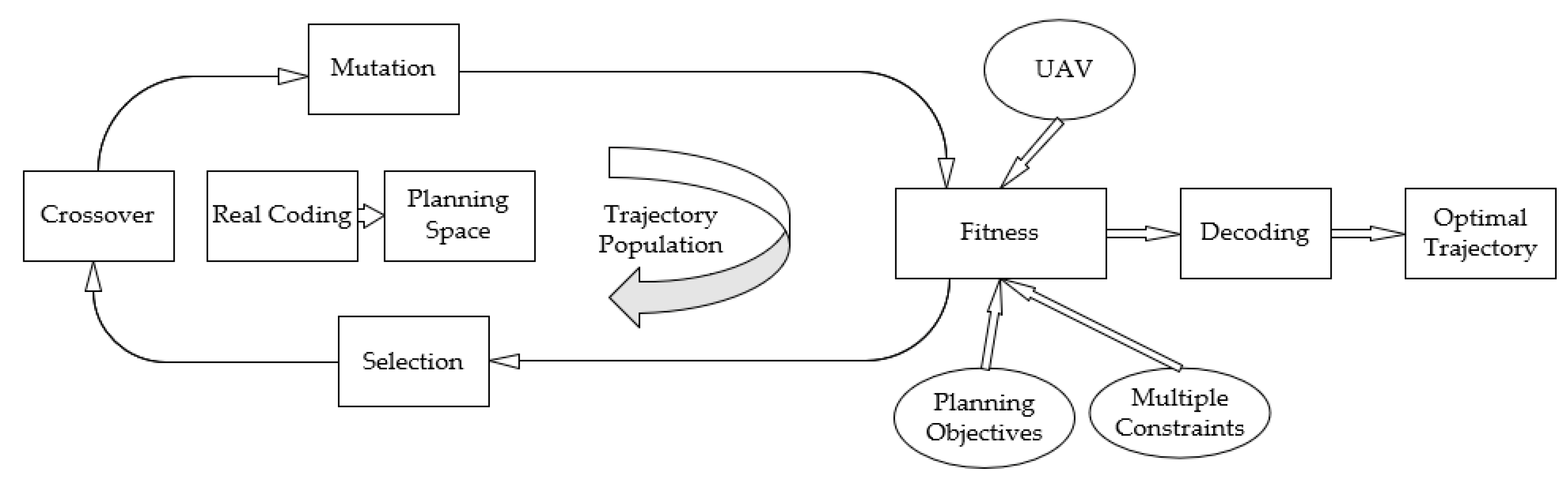
We have successfully established the objective function and constraints for Problem 1, and we will begin to solve it. The trajectory planning problem is a nonlinear programming problem with multiple constraints, which needs to consider the overall optimization, and to minimize the calculation amount while avoiding falling into a local optimum, and our study is to find the optimal flight path of an UAV from the starting point to the destination in three-dimensional space. Then we use the genetic algorithm. The basic idea of a genetic algorithm is to simulate the evolutionary process of biological genetics. Based on the principles of “survival of the fittest”, with the help of selection, crossing, and mutation, the problem to be solved approaches the optimal solution step by step from the initial solution. In trajectory planning, each chromosome (individual) of a genetic algorithm represents the trajectory of a UAV. The coding method of genes is also the coding method of trajectory nodes. The fitness function is changed by the cost function.

In this research, a UAV trajectory planning problem is combined with the idea of the genetic algorithm, and the real number gene coding method and specific genetic operator are used to meet the flight path trajectory of various constraint parameters to achieve the approximate optimal solution. The specific operation process is as follows:

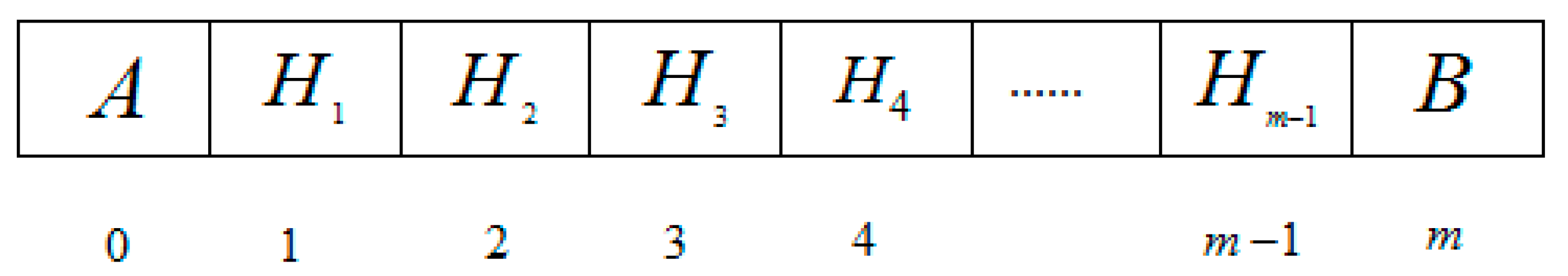
The first step: using the real number gene coding. Use the fixed-length real number gene coding method showed in Figure 3 to convert the position information of an UAV in three-dimensional space into the chromosomal gene structure (as shown in Figure 4). Each gene of the chromosome contains the three-dimensional spatial coordinate $\left(x,y,z\right)$ information of the gene, which records the following information of the spatial gene: one is whether the gene is feasible, and the other is whether the connecting line segment between the gene and the next gene is feasible. This gene sequence is only feasible if the above conditions are acceptable.

As can be seen from Figure 3, fixed-length real number gene coding is used to convert the position information of a UAV in three-dimensional space into the chromosomal gene structure, and the advantages of the fixed-length real number gene coding method are: one is to avoid increasing the number of the error correction points which let the coding length is too long, and the second is that in the genetic process, high frequency encoding and decoding operations are not required, the calculated amount is reduced, and the search efficiency of the algorithm is improved.

As for a UAV trajectory planning problem, each chromosome represents a complete sequence of trajectory points of a UAV, and this point sequence may or may not be feasible. Therefore, from the chromosome structure diagram of Figure 4, each chromosome contains information on the start and end positions, plus the gene composition H₁, H₂, H₃, …, H_n that does not repeat.

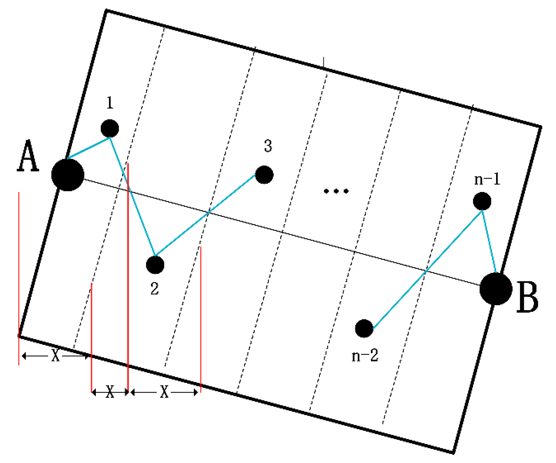
The second step: the initialization of the population. During the conversion of trajectory nodes to genetic algorithm chromosomes, in order to make the generated random nodes as close as possible to the planning area, the generated nodes can be evenly and effectively distributed in the planning space. In this research, we use a specific initialization method to complete the initialization work. It mainly uses a starting point and an ending point as the center of symmetry as a rectangular area, and the length of the rectangle is the length of the line connecting the starting point and the ending point, and the width is the length of the rectangle, and the rectangular area is the planning area. The planning area is evenly divided into m grids, and the trajectory nodes are uniformly generated in the planning area using a loop statement as shown in Figure 5:

Figure 5 shows the generation process of the trajectory node when i = 0: the starting point A to the ending point B can determine the slope of the line, and then find the function equation of the four sides of the area, use the Random function to generate the random number x of the specific area, and then in the three cases, the Random function is used again to combine the functions of the four sides to generate y, and then the height z of a UAV is generated within a specific range, thereby obtaining the first gene of the trajectory, which is calculated in turn, and will be obtained at that time. For the last gene of the trajectory, we save these genes one by one and form the gene sequence of the trajectory, then the gene sequence is a chromosome. In the next work, this method is used to cycle through, thus completing the entire trajectory initialization work.

The third step: determine the trajectory fitness function. Suppose that A can determine that the trajectory of B is represented by z₁, and its cost function is composed of optimization item $f_1\left(z_1\right)$ and penalty item $f_2\left(z_1\right)$, so:

$$f\left(z_1\right)=f_1\left(z_1\right)+f_2\left(z_1\right)$$

(15)

Among them, the optimization term of the trajectory cost function:

$$f_1\left(z_1\right)={\omega }_1\left[g_1\left(z_1\right)\right]+{\omega }_2\left[g_2\left(z_1\right)\right]$$

(16)

where $g_1\left(z_1\right)$ denotes the cost function value of the horizontal error on the arc of the trajectory A to B, $g_2\left(z_1\right)$denotes the cost function value of the vertical error on the arc of the trajectory A to B, ${\omega }_1$ represents the weight of the horizontal error in the total cost of the horizontal error and the vertical error, w₂ represents the weight of the vertical error in the total cost of the horizontal error and the vertical error, they should satisfy ${\omega }_1+{\omega }_2=1$ and the weight distributions of ${\omega }_1$and ${\omega }_2$ are similar.

The penalty of the trajectory cost function:

$$f_2\left(z_1\right)={\omega }_1\left[p_1\left(z_1\right)\right]+{\omega }_2\left[p_2\left(z_1\right)\right]$$

(17)

where $p_1\left(z_1\right)$ denotes the trajectory which the flight height of an UAV exceeds the maximum flight altitude of an UAV, $p_2\left(z_1\right)$ denotes the trajectory which an UAV trajectory length is greater than the maximum range of an UAV, $p_i$ denotes a penalty function for the i-th term, and ${\omega }_i$ denotes a penalty factor for the i-th term, i = 1, 2.

Take the trajectory fitness function:

$$fitness\left(z_1\right)=\frac{1}{f\left(z_1\right)}$$

(18)

where $f\left(z_1\right)$ represents the cost of the trajectory chromosome $z_1$, that is to say, the trajectory planning problem will be transformed from the cost minimization problem to the trajectory fitness maximization problem in genetic evolution.

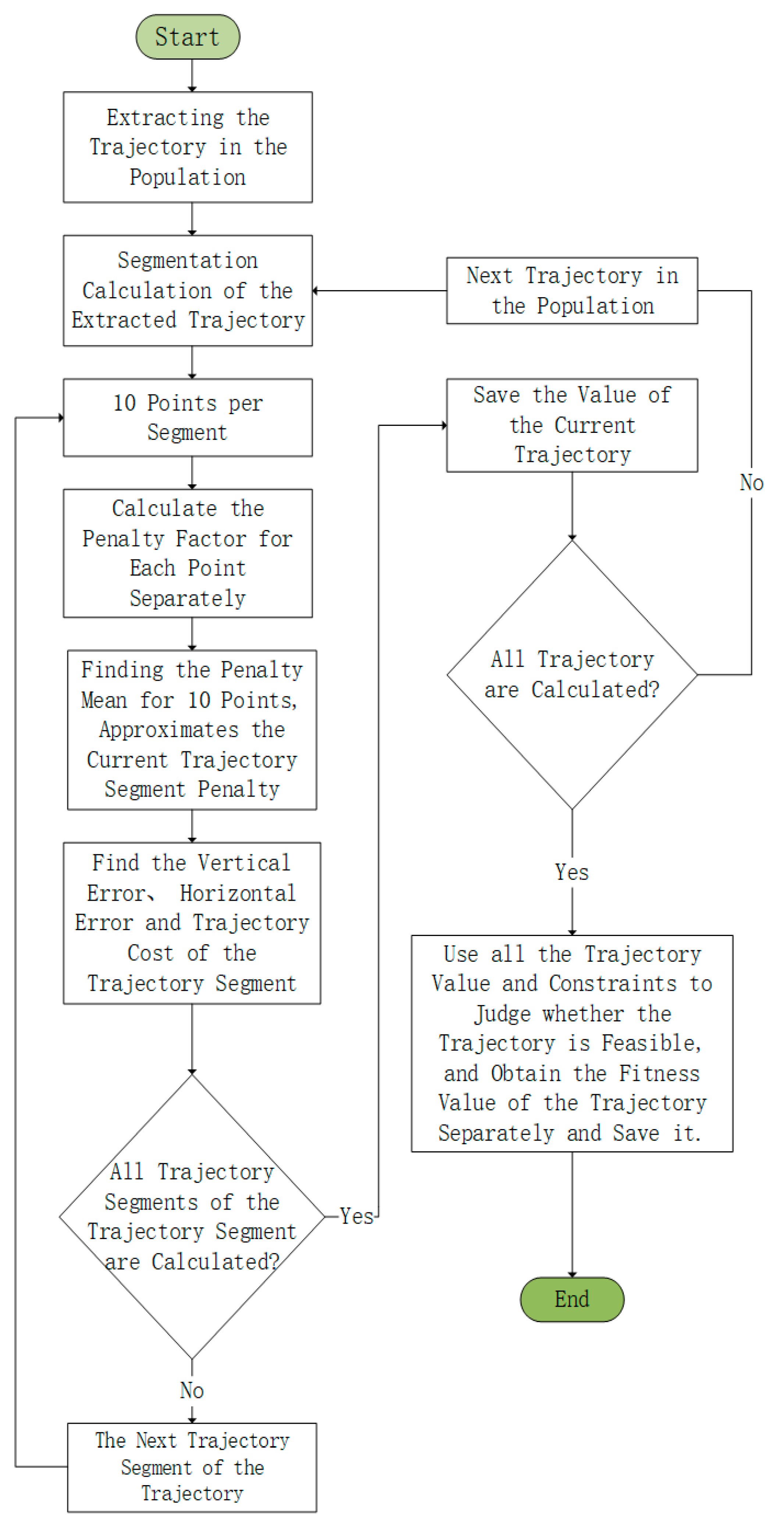
The fourth step: Solve the fitness value of the formula of the fitness function, as shown in Figure 6.

Figure 6 shows the process of solving the fitness value of the trajectory population. First, each trajectory in the population is extracted in turn, and the trajectory is segmented. Each trajectory is equally divided by 10 points, and the actual length of the trajectory segment and all penalty items is calculated. Ten points respectively ask for the penalty value and are accumulated for averaging. Then, calculate the length, vertical error, and horizontal error of the trajectory segment, and combine the constraints determined by the adjacent trajectory nodes to meet the requirements of each segment. Then, calculate the cost function and punishment for the trajectory segment. The values are accumulated. If the current trajectory is calculated, we need to save their value and penalty value separately, then calculate each trajectory in turn, and finally, when all the trajectories are calculated, find the fitness, which is the maximum value of the cost. The given constraints are used to determine if the trajectory is feasible and to save it.

The fifth step: determination of crossover probability and mutation probability. To prevent the genetic algorithm from converging prematurely, an improved adaptive genetic algorithm is used to solve the optimal flight path. The improved adaptive genetic algorithm adjusts the corresponding cross-probability $P_r$ and genetic probability $P_m$ according to the change of fitness during the evolution process. In the improved adaptive genetic algorithm, $P_r$and $P_m$are adaptively adjusted as follows:

$$P_r=\{\begin{array}{c}{P}_{r1}-\frac{\left(P_{r1}-P_{r2}\right)\left(f^{*}-\overline{f}\right)}{f_{\max }-\overline{f}},f^{*}\ge \overline{f}\\ P_{r1},f^{*}\le \overline{f}\end{array}$$

(19)

$$P_m=\{\begin{array}{c}{P}_{m1}-\frac{\left(P_{m1}-P_{m2}\right)\left(f-\overline{f}\right)}{f_{\max }-\overline{f}}\\ P_{m1},f\le \overline{f}\end{array},f\ge \overline{f}$$

(20)

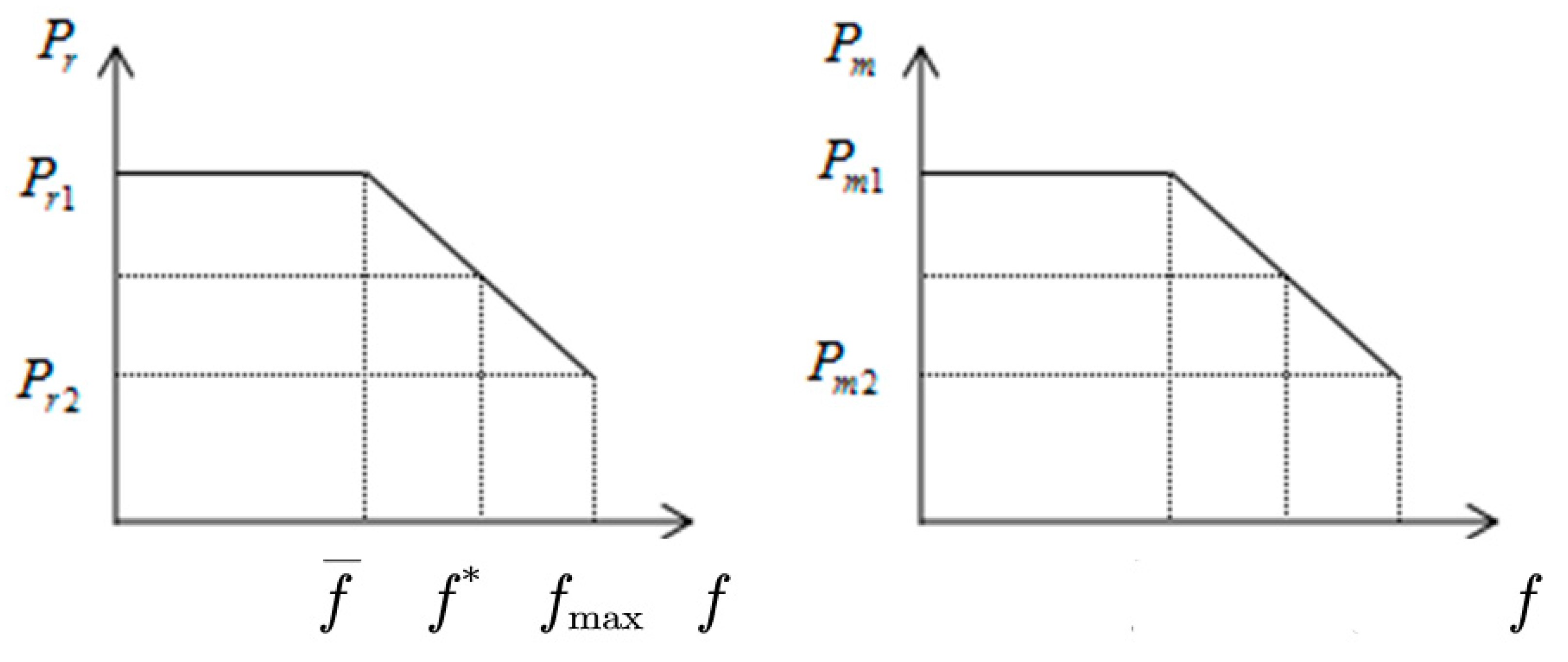
where $f_{\max }$ represents the maximum value of the population fitness, $\overline{f}$ represents the average value of the current population fitness, $f^{*}$ represents the fitness value of the larger of the two individuals currently used to cross, and $f$ represents the fitness value of the individual which needs to perform mutation operation. The improved adaptive genetic algorithm mainly makes the $P_r,P_m$ of the optimal individual in the early stage of evolution not zero, and it is not easy to fall into the local optimal solution, as shown in Figure 7:

Because adaptive adjustment may cause the population to fall into a local optimal solution, we adopt an improved method to improve $P_r,P_m$ so that the optimal individuals $P_r,P_m$ in the early evolution stage are not zero. The specific improvement process is to increase the population’s maximum fitness value $P_r$ to $P_{r1}$ and $P_m$ to $P_{m1}$. As shown in Figure 6, this will make the individual with the largest fitness value in the initial stage of evolution in a constant state, and check and mutate according to the size of $P_{r1}$, $P_{m1}$.

The above five steps are an UAV trajectory planning algorithm process of Problem 1. The overall algorithm flow can be expressed in Figure 8.

Figure 8 shows the combination of genetic algorithm and trajectory planning and the entire planning process. In Problem 1, we used the real number coding method to transform the trajectory planning problem into a genetic algorithm chromosome problem. Under multiple constraints and driven by the fitness function, the evolution operation of each generation is completed through operations such as genetic crossover and mutation, and finally decoded to obtain the required track node and complete the solution of the optimal solution for the trajectory planning.

3.3. Simulation Results and Analysis of the Trajectory Planning Algorithm for the Problem 1

According to the above algorithm, the results of the Problem 1 are calculated by using the data set.

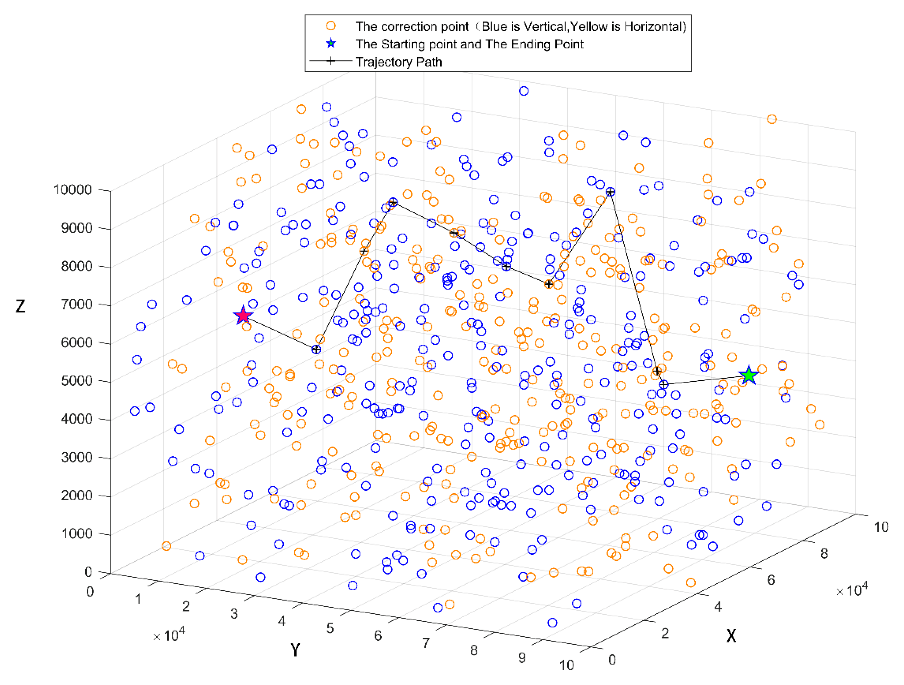
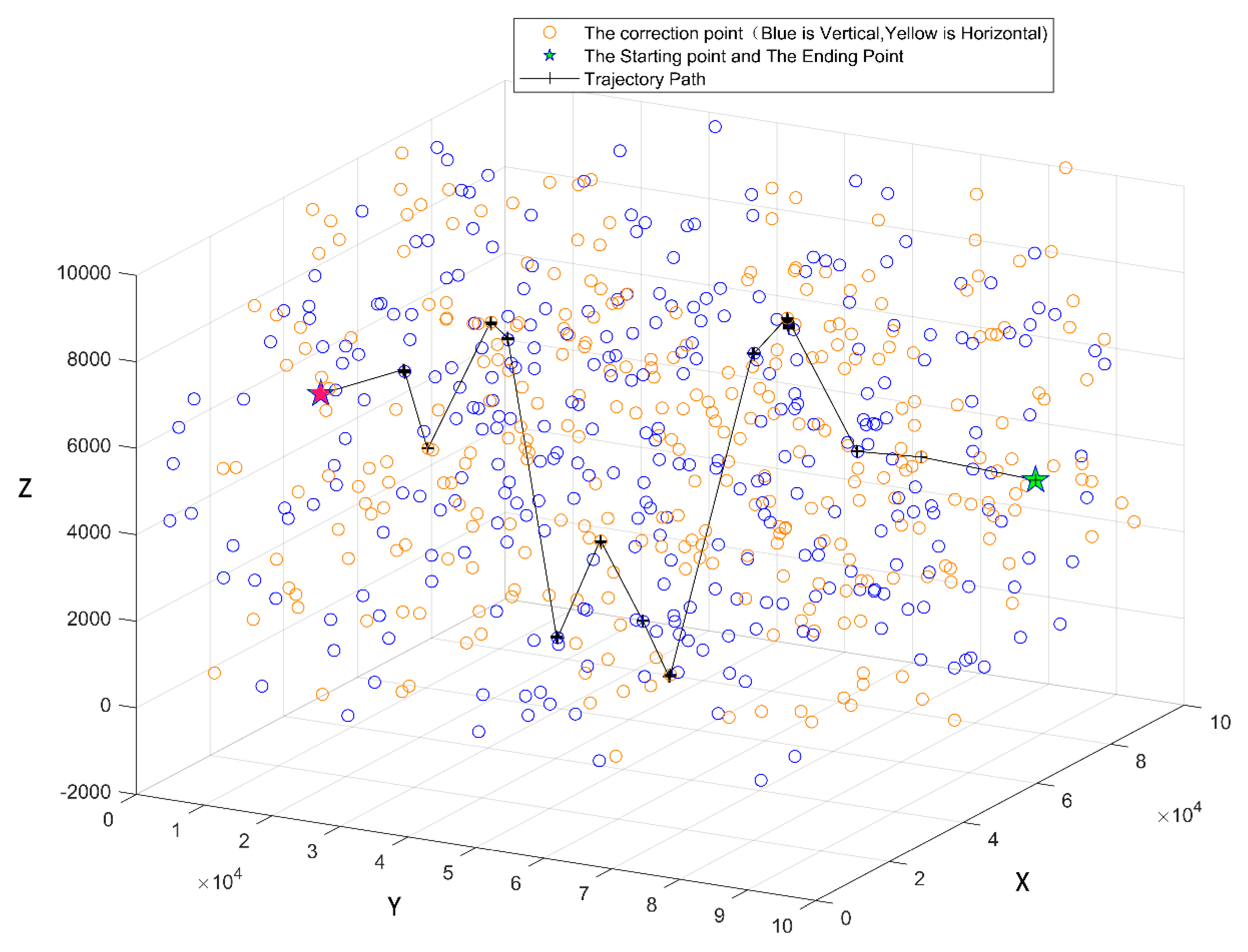
For the parameters of the data set, the vertical error and horizontal error will increase by δ dedicated units for each flight of 1 m; when a UAV reaches the ending point, the vertical error and horizontal error should be less than θ units; when vertical error correction is performed, the vertical error of an UAV is not more than α₁ units, and the horizontal error is not more than α₂ units; when the horizontal error correction is performed, the vertical error of an UAV is not more than β₁ units, and the horizontal error is not more than β₂ units. Under these parameters, we calculate the shortest path of the trajectory under the given constraint condition, and calculate the minimum number of times an UAV corrected by the correct area. The trajectory planning path map of the data set is shown in Figure 9.

Figure 9 shows the trajectory planning path of the data set. Firstly, the data of the data set is filtered and processed, and imported into MATLAB software. The discrete point maps of these three-dimensional spaces are drawn according to the type of correction points of an UAV. The mathematical model is established by given multiple constraints and designed objective function, and then the idea of genetic algorithm is used to analyze the feasibility of the horizontal error correction point and the vertical error correction point in the discrete point respectively. After the screening, through the fitness function, some fitness values are determined in turn, and the trajectory formed by the fitness function values is the optimal trajectory length.

Before determining the above-mentioned trajectory planning path and the number of times an UAV through the correct area for correction, the position of the corrected vertical and horizontal errors can be determined, and the error correction point number and the path planning of the error before the correction are obtained. The optimal trajectory length is 16,972.695304 m. The results are shown as

Table 2. Corrects result for Problem 1.

The Number of the Correction Points	The Type of the Correction Points
0	The Starting Point
504	1
295	0
124	1
76	0
34	1
12	0
404	1
595	0
398	1
612	The Ending Point

.

It can be seen from Table 2 that the shortest path to the trajectory set of the data set is according to the process of the above algorithm, that is, to initialize a gene, save these genes and form the gene sequence of the trajectory, then the gene sequence is a chromosome. Using this method to cycle back and forth, we can get a lot of chromosomes, then get the appropriate function value from the determined moderate function, and use the given constraints to determine whether the chromosome is feasible, to get the optimal trajectory length. On this basis, the number of times of correction of the correction area is calculated to be nine, and the error correction point number is obtained from the starting point.

4. Problem 2

In addition to the constraints including Problem 1, Problem 2 including the above-mentioned condition (8) in Section 2. That is to say, the condition that an UAV is restricted by the structure and control system when turning is unable to complete the instant turn. And, comprehensively consider the following optimization goals: (A) the trajectory length is as small as possible; (B) the number of corrections through the correct points is as small as possible.

If the above-mentioned parameters of the data are:

${\alpha }_1$ = 25, ${\alpha }_2$ = 15, ${\beta }_1$ = 20, ${\beta }_2$ = 25, $\theta$ = 30, $\delta$ = 0.001.

4.1. Multi-Constraints Optimization Problem

4.1.1. Objective Function

The focus of this research is to plan a trajectory for a UAV from the starting point to the ending point, and finding the optimal trajectory satisfied with the multi-constraints in Problem 2, so we build mathematical models of the problem.

$$F_1=\min ({\displaystyle \sum }_{i=1}^m({\eta }_i+{\lambda }_i+h_i+{\displaystyle \sum }_{1\le j\le i}{l}_j))$$

(21)

$$F_2=\min ({\displaystyle \sum }_{i=1}^m\left(a_i+b_i\right))$$

(22)

where F₁ represents the trajectory length of an UAV from the starting point A to the ending point B, F₂ represents the number of times an UAV has been corrected through the correction area, m represents the total number of corrections of an UAV throughout the flight, ${\eta }_i$ represents the distance of an UAV’s i-th flight, ${\lambda }_{i }$ represents the correction distance of the i-th flight to the vertical error correction point, $h_i$ represents the correction distance of the i-th flight to the horizontal error correction point, $l_j$ represents the distance that an UAV turns during the j-th flight, $a_i$ represents an UAV’s i-th flight reaches the vertical error correction point, and $b_i$represents an UAV’s i-th flight reaches the horizontal error correction point.

4.1.2. Multi-Constraints

The above objective function should satisfy the constraints of Problem 1 and the following constraints:

(1). When a UAV is flying from position $H_i$ to position $H_{i+1}$, due to the limitation of the UAV’s maneuverability, it will move in an arc segment $H_i{H}_{i+1}$. At this time, the circle is centered on the intersection of the mid-permanent line of the distance from position $H_i$ to position $H_{i+1}$ and the ideal trajectory of $H_i$ to$H_{i+1}$, so the radius $r_i$ can be expressed as:

$$r_i=\frac{{\eta }_i}{2}\cos \varphi ,i=1,\dots ,m$$

(23)

where ${\eta }_i$ represents the distance of an UAV which flies from position $H_i$ to position $H_{i+1}$,$r_i$ represents the turning radius of an UAV’s i-th flight, and$\varphi$ is the maximum yaw angle that an UAV is allowed to fly. During the flight of a UAV, it will be limited by the structure and control system, and it will not be able to complete the instant turn, so the turning distance of the j-th flight of an UAV can be obtained by:

$$l_j=\pi r_j-2r_j,1\le j\le i$$

(24)

(2). Due to the limitation of the UAV’s own maneuverability, a UAV can only turn within a certain range of yaw angle, that is, its yaw angle is less than or equal to the maximum allowed yaw angle before it can fly to the next trajectory point. The yaw angle limit is the minimum turning radius limit. The smaller the turning angle, the more smoothly a UAV can fly. Therefore, suppose the horizontal projection of the i-th trajectory segment is ${\gamma }_i=\left(x_i-x_{i-1},y_i-y_{i-1}\right)$, and the maximum yaw angle allowed by a UAV to fly is ϕ, then the constraint condition can be expressed as:

$$\cos \varphi \le \frac{{\gamma }_i{}^T{\gamma }_{i+1}}{\Vert {\gamma }_i\Vert \Vert {\gamma }_{i+1}\Vert },i=1, 2, \dots ,m$$

(25)

(3). A UAV is limited by the structure and control system during the turn and cannot complete the immediate turn. The minimum turning radius of an UAV is 200 m in Section 2.1, then the constraint condition can be expressed as:

$$200\le r_j\le \frac{{\eta }_j}{2}\frac{{\gamma }_i{}^T{\gamma }_{i+1}}{\Vert {\gamma }_i\Vert \Vert {\gamma }_{i+1}\Vert }, j=1,2,\dots ,i$$

(26)

In summary, the model for Problem 2 can be established as:

$$\begin{array}{c}{F}_1=\min ({\displaystyle {\displaystyle \sum }_{i=1}^m}({\eta }_i+{\lambda }_i+h_i+{\displaystyle {\displaystyle \sum }_{1\le j\le i}}{l}_j))\\ F_2=\min ({\displaystyle {\displaystyle \sum }_{i=1}^m}\left(a_i+b_i\right))\\ s.t.\{\begin{array}{c}{\displaystyle {\displaystyle \sum }_{i=1}^m}{a}_i{\eta }_i\delta <\theta \\ {\displaystyle {\displaystyle \sum }_{i=1}^m}{b}_i{\eta }_i\delta <\theta 0\le {\eta }_i\le l_{AB}\\ {\lambda }_i=a_i{\eta }_i\delta ,i=1,\dots ,m\\ h_i=b_i{\eta }_i\delta ,i=1,\dots ,m\\ a_i,b_i=0,1,i=1,\dots ,m\\ a_i+b_i=1,i=1,\dots ,m\\ {\lambda }_i\le {\alpha }_1,h_i\le {\alpha }_2,i=1,\dots ,m\\ {\lambda }_i\le {\beta }_1,h_i\le {\beta }_2,i=1,\dots ,m\\ l_j=\pi r_j-2r_j,\\ \cos \varphi \le \frac{{\gamma }_i{}^T{\gamma }_{i+1}}{\Vert {\gamma }_i\Vert \Vert {\gamma }_{i+1}\Vert },i=1,\dots ,m\\ 200\le r_j\le \frac{{\eta }_j}{2}\frac{{\gamma }_i{}^T{\gamma }_{i+1}}{\Vert {\gamma }_i\Vert \Vert {\gamma }_{i+1}\Vert },j=1,\dots ,m\end{array}\end{array}$$

(27)

4.2. Trajectory Planning Algorithm for the Problem 2

Problem 2 has a constraint on the minimum turning radius. Therefore, we adopt an improved sparse A* algorithm, which is an effective method to avoid useless trajectory nodes in space and reduce the time to search for feasible successor nodes. Using trajectory constraints to search only the effective space reduces the search space and speeds up the search. So, for Problem 2, we propose a trajectory planning problem based on the improved sparse A* algorithm. First, we plan the division of space. Attention should be paid to reducing the number of divided cells as much as possible, thereby reducing the amount of calculation and improving the algorithm’s convergence speed, so that the algorithm can plan the feasible trajectory of a UAV in the shortest time. Then, there is the determination of the cost function.

If $g\left(n\right)$ represents the actual cost of a UAV at the current trajectory node n in space:

$$g\left(n\right)=q_1{R}_n\left(P\right)+q_2{S}_n\left(P\right)$$

(28)

where R,S represents the flight cost of a UAV respectively, the horizontal and vertical error correction costs of a UAV, and $q_1,q_2$each represent the weight coefficient of R,S.

$$R_n={\displaystyle \sum }_{i=1}^m{\eta }_i$$

(29)

$$S_n={\displaystyle \sum }_{i=1}^m\left(a_i+b_i\right){\eta }_i\delta$$

(30)

where ${\eta }_i$ represents the distance of an UAV’s i-th flight, $a_i$ represents an UAV’s i-th flight to the vertical correction point, b_i represents an UAV’s i-th flight to the horizontal correction point, and $\delta$ indicates that the horizontal error and vertical error increase by $\delta$ units each time an UAV flies 1 metre. Let $h\left(n\right)$ represent the Euclidean distance from the current trajectory node to the target trajectory node $B\left(x_B,y_B,z_B\right)$, and $q_3$ represent the weight coefficient of $h\left(n\right)$, then:

$$h\left(n\right)=\sqrt{{\left(x_n-x_B\right)}^2+{\left(y_n-x_B\right)}^2+{\left(z_n-x_B\right)}^2}$$

(31)

Therefore, the improved cost function f(n) can be determined as:

$$f\left(n\right)=q_1{R}_n\left(P\right)+q_2{S}_n\left(P\right)+q_{3}h\left(n\right)$$

(32)

A UAV’s online real-time trajectory planning task requires an improved sparse algorithm to complete the trajectory planning in a short time and a small memory space. The node can be expanded by an improved cost function, nodes can be expanded with an improved cost function, using two linked lists, of which the open table stores the nodes to be expanded, and the close table stores the nodes already. The specific algorithm flow is as follows and can be seen in Figure 10:

Step 1: The search space is divided according to the requirements of the aircraft for the accuracy of the trajectory.

Step 2: Put the starting point A into the open table, and the closing table is initially empty.

Step 3: If the open table is empty, it means that the search failed, and the algorithm exited.

Step 4: Remove the least costly trajectory node in the open table as the current trajectory node, and store the point in the closing table.

Step 5: If the current node is midpoint B, the search is ended, and the algorithm exits successfully. Starting from point B and going back to point A, we get the optimal path from point A to point B. Otherwise, go to the next step.

Step 6: The successor node of the node with the least expansion cost. Point the parent pointer of the succeeding node to the node with the least cost.

Step 7: Calculate the generation value of the successor node according to the improved cost function formula, and insert the successor node into the open table according to the generation value.

Step 8: Return to step 3.

Step 6 is to classify the successor nodes of the node with the least expansion point cost as follows:

The first type: If the successor node already exists in the open table, the successor node is discarded; the node is added to the node table with the least cost; and then calculate and compare the actual cost g value of the point, determine whether the parent node of the point needs to be relocated, and if so, update the generation value;

The second type: If the subsequent node is in the closing table, call the Step 7 to calculate the path cost. If it is smaller, update the total generation value f and actual generation value g of the parent node. If find that there is a better path to reach this point in the path search, extend this step to the subsequent nodes of this point;

The third type: If the successor node is not in the open table and the closing table, then the node is placed in the open table.

4.3. Simulation Results and Analysis of the Trajectory Planning Algorithm for the Problem 2

According to the above algorithm, the results of the Problem 2 are calculated by using the data set. As the Problem 2 is based on the Problem 1, considering that an UAV is limited by the structure and control system when turning, it cannot complete the instant turn. According to the Problem 2, the minimum turning radius of the aircraft is 200 m. Then, use the improved A* algorithm to calculate its maximum yaw angle, and use MATLAB software to make a path planning path map of the data set. Figure 11 shows the trajectory planning path map of an UAV.

Figure 11 shows that both the horizontal error correction point and the vertical error correction point are evenly distributed in the three-dimensional space. This question considers that when a UAV turns from the current trajectory node in the horizontal direction to the next trajectory node, due to the limitations of the UAV’s own performance, it can only turn within a certain yaw angle range. Therefore, through the above algorithm, the feasible correction point is searched in turn. Connect these feasible correction points, that is, get a trajectory planning path, use this method to cycle back and forth, which constitutes the optimal trajectory length in Figure 11.

Under the constraint condition that a UAV is turning within a certain yaw angle, the position of the trajectory planning path and the number of times a UAV passes the correct area for correction can be determined before the correction of the vertical and horizontal errors, and a UAV starts from the starting point. The error correction point number and the trajectory planning result table of the error before correction are shown in

Table 3. Corrects result for Problem 2.

The Number of the Correction Points	The Type of the Correction Points
0	The Starting Point
346	1
200	0
294	0
136	1
108	1
74	0
462	1
543	0
369	1
457	0
388	1
436	0
612	The Ending Point

.

Obtaining the optimal trajectory length from starting point to ending point is 14957.842315 m. From the table, the number of times of correction of the correction area is calculated 12 times, and the error correction point number passing through the starting point from the starting point is obtained.

5. Performance Comparison of the Proposed Algorithm with Traditional Swarm Intelligence Algorithm

5.1. For the Problem 1

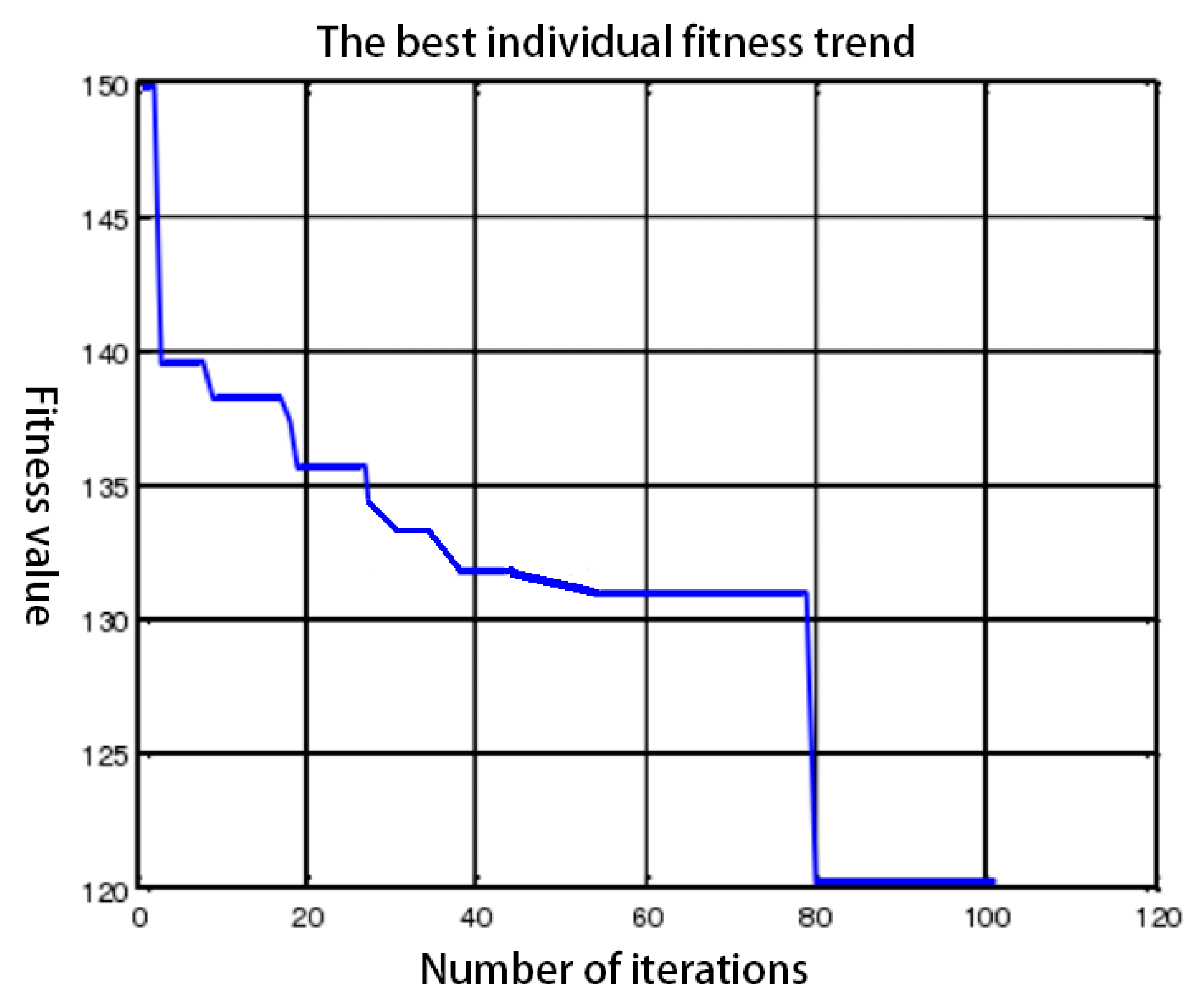
For the data set, we compare the proposed improved GA algorithm with the traditional GA algorithm in trajectory planning. Figure 12 shows the fitness change of traditional GA algorithm:

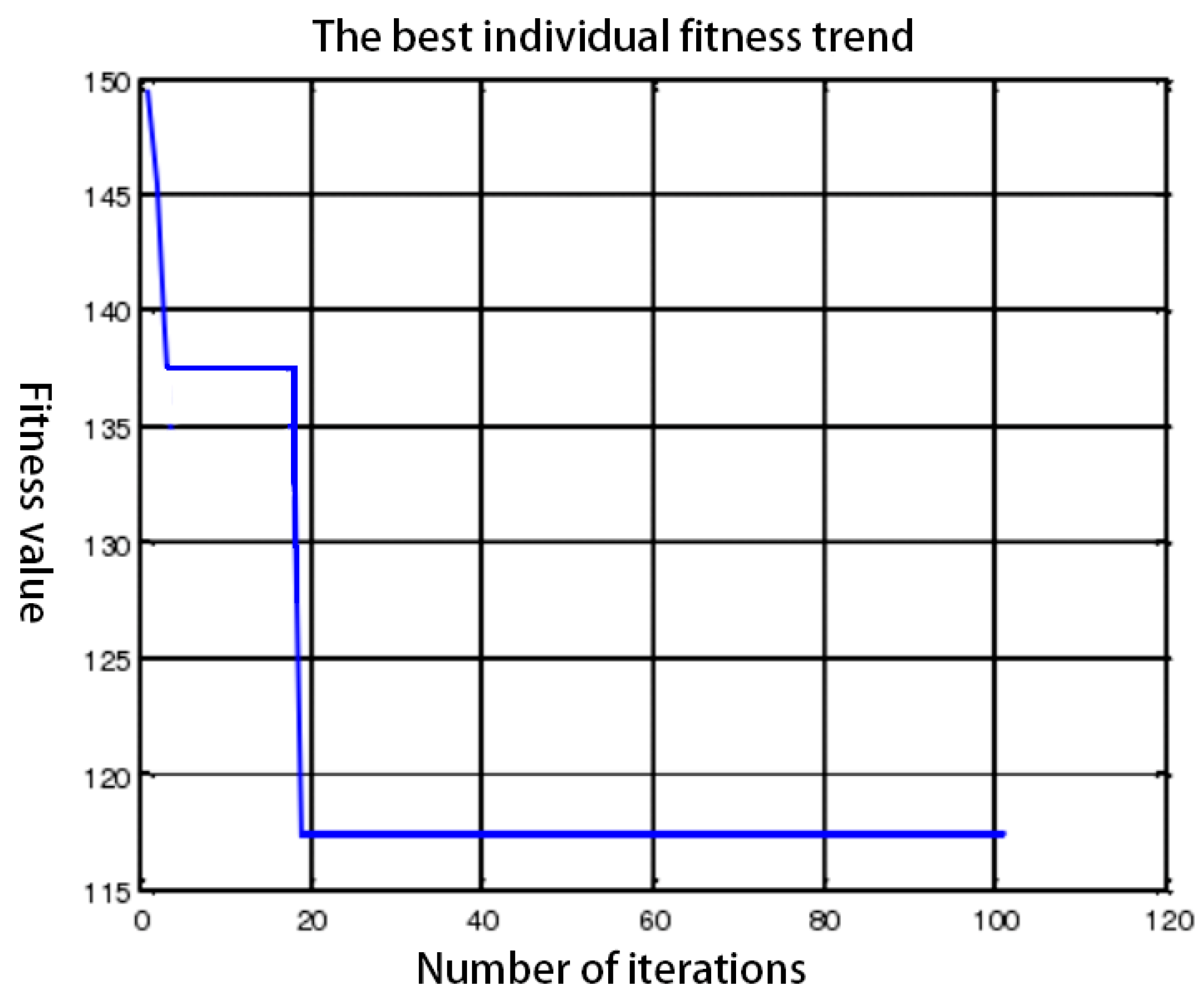
Figure 13 shows the fitness change of the proposed improved GA algorithm:

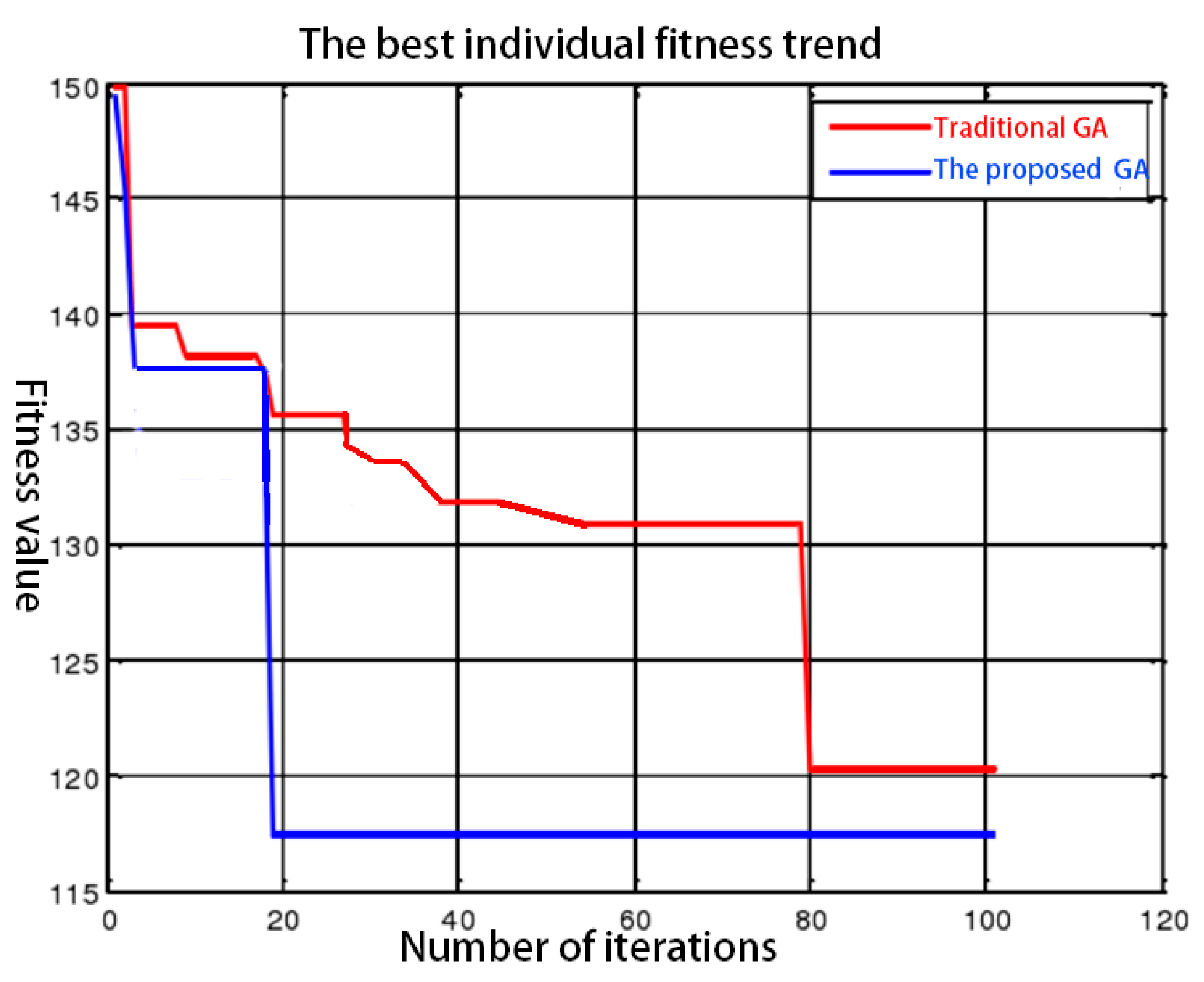
In order to compare the performance of the two algorithms more clearly, draw the fitness curves of Figure 12 and Figure 13 into a unified coordinate system, as shown in Figure 14:

It can be seen from Figure 14 that: (1) the proposed improved GA algorithm converges significantly faster than the traditional GA algorithm, (2) the proposed improved GA algorithm has a lower overall cost for the optimal trajectory search, (3) during the search of the proposed improved GA algorithm, the shock is small. Therefore, the proposed improved GA algorithm in the paper is significantly better than the traditional GA algorithm.

5.2. For the Problem 2

Experiments were performed using the basic A* algorithm and the improved A* algorithm, and the superiority of the algorithm was verified by comparing the path length of the trajectory planning and the number of correction points passed. Using the data set, the two weight coefficients $q_1,q_2$ and $q_3$of Formula (32) are set, respectively, as shown in

Table 4. The weight coefficient of the improved cost function $f\left(n\right)$.

Number	q1	q2	q3
1	0.3	0.2	0.5
2	0.3	0.5	0.2

.

In the course of trajectory selection, the smaller the value of the cost function, the better the trajectory.

Table 5. Performance comparison of A* algorithm and the proposed improved sparse A* algorithm.

Number	Algorithm	Number of Correction Points Passed	Trajectory Length
1	Before improvement	31	35,436.632176
	After improvement	12	14,957.842315
2	Before improvement	39	41,258.581392
	After improvement	15	19,513.452647

compares the experimental performance of the proposed improved sparse A* algorithm and the basic A* algorithm in the same environment.

In Table 5, before improvement means that the basic A* algorithm, and after improvement means that the proposed improved sparse A* algorithm in this paper is used. Numbers 1 and 2 represent the weight coefficients of numbers 1 and 2 in Table 4. It can be seen from Table 5 that the larger $q_2$ is, the larger correction points are passed, and the larger $q_3$ is, the shorter the trajectory length is. Therefore, the values of these weighting factors can be adjusted from different needs. Furthermore, it can be seen that the performance of the improved sparse A* algorithm is significantly better than the basic A* algorithm.

6. Conclusions

The proposed method allows for multiple constraints optimal trajectory planning using the improved genetic algorithm (GA) and A* algorithm. The conclusions of this research work are: (1) The numerical results of the experiment proved that the improved genetic algorithm (GA) and A* algorithm are good for optimal trajectory planning. (2) All essential constraints like the correction and turning radius of a UAV are satisfied with all solutions obtained from the trajectory planning algorithm.

Future work should take into account more complex and realistic constraints, such as threats to the ground or in the air, the avoidance of obstacles, and other constraints of the UAV itself (such as its own battery life), improve the algorithm optimization model and objective functions (such as considers flight time [28]), and ensure that UAVs are able to adapt to more complex environments.

References

- Zhao, S.Y.; Hu, Z.Y.; Chen, B.M.; Lee, T.H. A Robust Real-Time Vision System for Autonomous Cargo Transfer by an Unmanned Helicopter. IEEE Trans. Ind. Electron. 2015, 62, 1210–1218. [Google Scholar] [CrossRef]
- Shen, Y.F.; Rahman, Z.; Krusienski, D.; Li, J. A vision-based automatic safe landing-site detection system. IEEE Trans. Aerosp. Electron. Syst. 2013, 49, 294–311. [Google Scholar] [CrossRef]
- Huh, S.; Cho, S.; Jung, Y.; Shim, D.H. Vision-based sense-and-avoid framework for unmanned aerial vehicles. IEEE Trans. Aerosp. Electron. Syst. 2015, 51, 3427–3439. [Google Scholar] [CrossRef]
- ElMikaty, M.; Stathaki, T. Car Detection in Aerial Images of Dense Urban Areas. IEEE Trans. Aerosp. Electron. Syst. 2018, 54, 51–63. [Google Scholar] [CrossRef]
- Zhao, L.; Wang, D.; Huang, B.; Xie, L. Distributed Filtering-Based Autonomous Navigation System of UAV. Unmanned Syst. 2015, 3, 17–34. [Google Scholar] [CrossRef]
- Carrillo, L.R.G.; Fantoni, I.; Rondon, E.; Dzul, A. Three-dimensional position and velocity regulation of a quad-rotorcraft using optical flow. IEEE Trans. Aerosp. Electron. Syst. 2015, 51, 358–371. [Google Scholar] [CrossRef] [Green Version]
- Kaiser, M.K.; Gans, N.R.; Dixon, W.E. Vision-Based Estimation for Guidance, Navigation, and Control of an Aerial Vehicle. IEEE Trans. Aerosp. Electron. Syst. 2010, 46, 1064–1077. [Google Scholar]
- Khatib, O. Real-time obstacle avoidance for manipulators and mobile robots. Int. J. Robot. Res. 1986, 5, 90–99. [Google Scholar] [CrossRef]
- Chazelle, B.; Edelsbrunner, H. An improved algorithm for constructing kth-order Voronoi diagrams. IEEE Trans. Comput. 1987, 100, 1349–1354. [Google Scholar] [CrossRef]
- Li, Q.Q.; Zhe, Z. A Voronoi-based hierarchical graph model of road network for route planning. In Proceedings of the 11th Conference Intelligent Transportation Systems, Beijing, China, 12–15 October 2008; pp. 599–604. [Google Scholar]
- Sugihara, K. Approximation of generalized Voronoi diagrams by ordinary Voronoi diagrams. Cvgip Graph. Models Image Process. 1993, 55, 522–531. [Google Scholar] [CrossRef]
- Meng, B.B.; Gao, X.G. UAV Path Planning Based on Bidirectional Sparse A* Search Algorithm. In Proceedings of the 2010 International Conference on Intelligent Computation Technology and Automation (ICICTA), Changsha, China, 11–12 May 2010. [Google Scholar]
- Szczerba, R.J.; Galkowski, P.; Glicktein, I.S.; Ternullo, N. Robust algorithm for real-time route planning. IEEE Trans. Aerosp. Electron. Syst. 2000, 36, 869–878. [Google Scholar] [CrossRef] [Green Version]
- Chen, X.; Chen, X.M.; Zhang, J. The Dynamic Path Planning of UAV Based on A* Algorithm. Appl. Mech. Mater. 2014, 494–495, 1094–1097. [Google Scholar] [CrossRef]
- Wang, H.; Zhou, H.; Yao, H. Research on autonomous planning method based on improved quantum Particle Swarm Optimization for Autonomous Underwater Vehicle. In Proceedings of the OCEANS 2016 MTS/IEEE, Monterey, CA, USA, 19–23 September 2016. [Google Scholar]
- Zhang, H.; Liu, Z. 3D path planning for micro air vehicles based on quantum-behaved particle swarm optimization algorithm. J. Cent. South Univ. 2013, 44, 58–62. [Google Scholar]
- Tokgo, M.; Li, R. Estimation Method for Path Planning Parameter Based on a Modified QPSO Algorithm. In Proceedings of the International Conference on Artificial Intelligence: Methodology, Systems, and Applications, Varna, Bulgaria, 11–13 September 2014. [Google Scholar]
- Shorakaei, H.; Vahdani, M.; Imani, B.; Gholami, A. Optimal cooperative path planning of unmanned aerial vehicles by a parallel genetic algorithm. Robotica 2016, 34, 823–836. [Google Scholar] [CrossRef]
- Men, J.Z.; Qun, E.; Yao, K.M. Study on the Route Planning for Anti-Submarine Ship-Based UAV Based on Genetic Algorithm. Adv. Mater. Res. 2012, 433–440, 4823–4826. [Google Scholar] [CrossRef]
- Zhang, D.Q.; Zhao, J.F.; Lei, G.; Wang, S.H.; Zheng, X.L. Hurry Path Planning Based on Adaptive Genetic Algorithm. Appl. Mech. Mater. 2014, 446–447, 1292–1297. [Google Scholar] [CrossRef]
- Shiri, H.; Park, J.; Bennis, M. Massive Autonomous UAV Path Planning: A Neural Network Based Mean-Field Game Theoretic Approach; Cornell University: Ithaca, NY, USA, 2019. [Google Scholar]
- Hao, Z.; Cao, C.; Xu, L.; Gulliver, T.A. AN UAV Detection Algorithm Based on an Artificial Neural Network. IEEE Access 2018, 6, 24720–24728. [Google Scholar]
- Chen, Y.B.; Luo, G.C.; Mei, Y.S.; Yu, J.Q.; Su, X.L. UAV path planning using artificial potential field method updated by optimal control theory. Int. J. Syst. Sci. 2016, 47, 1407–1420. [Google Scholar] [CrossRef]
- Xia, C.; Jing, Z. The Three-Dimension Path Planning of UAV Based on Improved Artificial Potential Field in Dynamic Environment. In Proceedings of the International Conference on Intelligent Human-Machine Systems & Cybernetics, Hangzhou, China, 26–27 August 2013. [Google Scholar]
- Liu, J.Y.; Guo, Z.Q.; Liu, S.Y. The Simulation of an UAV Collision Avoidance Based on the Artificial Potential Field Method. Adv. Mater. Res. 2012, 591–593, 1400–1404. [Google Scholar] [CrossRef]
- Meng, H.; Xin, G. UAV route planning based on the genetic simulated annealing algorithm. In Proceedings of the IEEE International Conference on Mechatronics and Automation, Xi’an, China, 4–7 August 2010; pp. 788–793. [Google Scholar]
- China Ministry of Education Degree and Graduate Education Development Center. Available online: https://cpipc.chinadegrees.cn/ (accessed on 19 September 2019).
- Kwasniewski, K.K.; Gosiewski, Z. Genetic Algorithm for Mobile Robot Route Planning with Obstacle Avoidance. Acta Mech. Autom. 2018, 12, 151–159. [Google Scholar] [CrossRef] [Green Version]
Figure 1.
Schematic diagram of an UAV trajectory planning area. The yellow points are the horizontal error correction point, the blue points are the vertical error correction point, the starting point is point A, and the destination is point B. The black curve represents a trajectory.
Figure 2.
The physical space and the correct point. The blue point is the vertical error correction point, the yellow point is the horizontal error correction point, the red pentagram indicates starting point, the green pentagram indicates ending points. The range of axes comes from the data set.
Figure 3.
Fixed-length real-valued gene.
Figure 4.
Chromosome structure.
Figure 5.
Trajectory initialization principle.
Figure 6.
Solution process of trajectory fitness value.
Figure 7.
Improved adaptive crossover probability and mutation probability.
Figure 8.
Flow chart of an UAV trajectory planning algorithm based on an improved genetic algorithm.
Figure 9.
Trajectory planning path for the Problem 1.
Figure 10.
Flow chart of the improved sparse A* algorithm.
Figure 11.
Trajectory planning path for the Problem 2.
Figure 12.
Fitness curve of traditional GA algorithm for the Problem 1.
Figure 13.
Fitness curve of the proposed improved GA algorithm for the Problem 1.
Figure 14.
Two algorithms for fitness.