Localization of Small Anomalies via the Orthogonality Sampling Method from Scattering Parameters

Abstract

We investigate the application of the orthogonality sampling method (OSM) in microwave imaging for a fast localization of small anomalies from measured scattering parameters. For this purpose, we design an indicator function of OSM defined on a Lebesgue space to test the orthogonality relation between the Hankel function and the scattering parameters. This is based on an application of the Born approximation and the integral equation formula for scattering parameters in the presence of a small anomaly. We then prove that the indicator function consists of a combination of an infinite series of Bessel functions of integer order, an antenna configuration, and material properties. Simulation results with synthetic data are presented to show the feasibility and limitations of designed OSM.

1. Introduction

Localization or imaging of unknown targets from measured scattered fields or scattering parameter data is an old but interesting inverse scattering problem. This problem has a wide range of applications, for example, breast-cancer detection in biomedical imaging [1,2,3], anti-personnel mine detection, synthetic aperture radar (SAR), ground penetrating radar (GPR) in geoscience and remote sensing [4,5,6], and damage detection in civil structures [7,8,9]. We also refer to [10,11,12] for various applications of the inverse scattering problem.

Various techniques for solving this problem have been developed mostly based on iterative schemes, e.g., the Newton or Gauss-Newton, Levenberg-Marquadt, level-set, and optimal control approaches ([13], Table II). It is well known that the successful performance of an iteration-based scheme depends strongly on starting the iteration procedure with a good initial guess [14,15]. Therefore, generating a good initial guess close to the unknown target must be considered before the beginning of the iteration process. Various non-iterative algorithms have been investigated for this purpose and successfully applied to various inverse scattering problems.

The orthogonality sampling method (OSM) has been investigated recently in connection with the problem of localizing small targets and imaging the geometric features of arbitrarily shaped ones (compared to the operating wavelength) from measured scattered fields or far-field data. Pioneering research [16] has confirmed that OSM is a simple and stable technique, capable of perceiving an outline shape of small targets within a single incident field. In addition, OSM has been applied and extended to various inverse scattering problems, for example, multi-frequency imaging [17], the near-field orthogonality sampling method (NOSM) [18] and its improvement [19], three-dimensional problems modeled by Maxwell’s equations [20], and identification of sound-soft arcs in limited-aperture inverse acoustic problems [21]. Moreover, new imaging capability of OSM has been investigated in [22], and NOSM was successfully applied to cross-borehole ground penetrating radar (GPR) imaging [23].

Various non-iterative techniques were also applied recently to microwave imaging when the measurement data are scattering parameters (S-parameters). Examples include the MUltiple SIgnal Classification (MUSIC) algorithm [24], subspace migration [25], Kirchhoff migration [26], and direct sampling method [27]. Among them, subspace migration [28], direct sampling method [29], and factorization method [30] were applied to real-world microwave imaging. However, little research was conducted regarding the application of OSM to microwave imaging when the measurement data are S-parameters. This provides motivation for research on the application of OSM in microwave imaging and analysis of the indicator function for determining its feasibility and limitations.

The purpose of this paper is to design an indicator function of OSM for localizing small anomalies from measured S-parameters with a single transmitter and explore the mathematical structure of that indicator function by constructing a relationship with an infinite series of Bessel functions of integer order of the first kind, an antenna configuration, and material properties of the anomalies. This is based on the analytical expression of the integral representation formula for the scattered field S-parameters in the presence of anomalies [31] and application of the Born approximation [32]. From the explored structure of the indicator function, we can investigate whether the imaging performance of designed indicator function is significantly influenced by the antenna configuration (total number and array), material properties of anomalies (size, permittivity, and conductivity), and the location of the transmitter.

The remainder of this paper is organized as follows. Section 2 introduces the basic concept and integral equation formula for the scattered field S-parameters and describes the design of the indicator function of OSM. Section 3 presents a mathematical analysis of the structure of the designed indicator function and examines the feasibility and limitations of OSM in microwave imaging. Section 4 exhibits several simulation results with synthetic data that support the theoretical results. Section 5 contains a short conclusion and draws a future work.

Let us underline that some non-iterative algorithms such as MUSIC and subspace migration are also based on orthogonality relations between measurement data and an appropriate test function. However, the biggest difference from OSM is that a large number of incident fields with various directions are needed to apply, refer to [33,34,35,36,37]. Since OSM requires either one or a small number of fields with incident directions, obtained results via OSM will be poorer than MUSIC and subspace migration. Investigation of a detailed relationship between OSM and existing methods is interesting and important, but it lies outside the scope of this research.

2. Scattered Field S-Parameters and Indicator Function of Orthogonality Sampling Method

2.1. Maxwell’s Equation and Scattered Field S-Parameters

Let $\mathsf{\Omega }$ be the region of interest (ROI) and $\mathsf{\Sigma }\subset \mathsf{\Omega }$ a small anomaly enclosed by a simple circular array consisting of N transmitting (Tx)—receiving (Rx) dipole antennas ${\mathbf{d}}_n$, $n=1,2,\cdots ,N$. Throughout this paper, we assume that $\mathsf{\Sigma }$ can be represented as

$$\mathsf{\Sigma }={\mathbf{r}}_{★}+\rho \mathbf{B},$$

where ${\mathbf{r}}_{★}$ and $\rho$ characterize the location and the size, respectively, and $\mathbf{B}$ denotes a simply connected domain that describes the shape of $\mathsf{\Sigma }$.

Throughout this paper, we assume that the background medium and anomaly are non-magnetic. This implies that the value of the magnetic permeability is constant $\mu (\mathbf{r})={\mu }_{\mathrm{b}}\equiv 1.256\times {10}^{-6}\mathrm{H}/\mathrm{m}$ and, correspondingly, that they are characterized by the values of their dielectric permittivity and electrical conductivity at a given angular frequency $\omega =2\pi f$. We designate ${\epsilon }_{★}={\epsilon }_{\mathrm{r}★}·{\epsilon }_0$ and ${\epsilon }_{\mathrm{b}}={\epsilon }_{rb}·{\epsilon }_0$ as the permittivity of $\mathsf{\Sigma }$ and the background, respectively. Here, ${\epsilon }_0=8.854\times {10}^{-12}\mathrm{F}/\mathrm{m}$ is the vacuum permittivity. Conductivities ${\sigma }_{★}$ and ${\sigma }_{\mathrm{b}}$ can be defined analogously. Given these facts, we introduce the piecewise constant permittivity $\epsilon (\mathbf{r})$ and conductivity $\sigma (\mathbf{r})$ as follows:

$$\epsilon (\mathbf{r})=\left\{\begin{array}{ccc}\hfill {\epsilon }_{★}& \mathrm{if}& \mathbf{r}\in \mathsf{\Sigma },\hfill \\ \hfill {\epsilon }_{\mathrm{b}}& \mathrm{if}& \mathbf{r}\in \mathsf{\Omega }\backslash \overline{\mathsf{\Sigma }},\hfill \end{array}\right.\mathrm{and}\sigma (\mathbf{r})=\left\{\begin{array}{ccc}\hfill {\sigma }_{★}& \mathrm{if}& \mathbf{r}\in \mathsf{\Sigma },\hfill \\ \hfill {\sigma }_{\mathrm{b}}& \mathrm{if}& \mathbf{r}\in \mathsf{\Omega }\backslash \overline{\mathsf{\Sigma }},\hfill \end{array}\right.$$

respectively. For the sake, we assume that ${\epsilon }_{★}>{\epsilon }_{\mathrm{b}}>0$ and ${\sigma }_{★}>{\sigma }_{\mathrm{b}}>0$. With this, we designate k as the background wavenumber that satisfies

$$k^2={\omega }^2{\mu }_{\mathrm{b}}\left({\epsilon }_{\mathrm{b}}+i\frac{{\sigma }_{\mathrm{b}}}{\omega }\right).$$

The measurement data are scattered field S-parameters between a fixed transmitter m and receiver n, say, $\left\{{\mathrm{S}}_{scat}(n,m):n=1,2,\cdots ,N\right\}$, where ${\mathrm{S}}_{scat}(n,m)$ is obtained by subtracting the S-parameters with and without an anomaly $\mathsf{\Sigma }$, refer to [24,27,28,29,31,38]. On the basis of [31], ${\mathrm{S}}_{scat}(n,m)$ is given by the following integral equation formula

$${\mathrm{S}}_{scat}(n,m)=\frac{i{k}^2}{4\omega {\mu }_{\mathrm{b}}}{\int }_{\mathsf{\Omega }}\chi (\mathbf{r}){\mathbf{E}}_{inc}({\mathbf{d}}_m,\mathbf{r})·{\mathbf{E}}_{tot}(\mathbf{r},{\mathbf{d}}_n)d\mathbf{r},$$

(1)

where $\chi (\mathbf{r})$ is the objective function

$$\chi (\mathbf{r})=\frac{\epsilon (\mathbf{r})-{\epsilon }_b}{{\epsilon }_{\mathrm{b}}}+i\frac{\sigma (\mathbf{r})-{\sigma }_{\mathrm{b}}}{\omega {\epsilon }_{\mathrm{b}}},$$

$\mathbf{H}$ is the magnetic field, ${\mathbf{E}}_{inc}({\mathbf{d}}_m,\mathbf{r})$ is the incident electric field in a homogeneous medium due to the point current density at ${\mathbf{d}}_m$

$$\nabla \times {\mathbf{E}}_{inc}({\mathbf{d}}_m,\mathbf{r})=-i\omega {\mu }_{\mathrm{b}}\mathbf{H}({\mathbf{d}}_m,\mathbf{r})\mathrm{and}\nabla \times \mathbf{H}({\mathbf{d}}_m,\mathbf{r})=({\sigma }_{\mathrm{b}}+i\omega {\epsilon }_{\mathrm{b}}){\mathbf{E}}_{inc}({\mathbf{d}}_m,\mathbf{r}),$$

and ${\mathbf{E}}_{tot}(\mathbf{r},{\mathbf{d}}_n)$ is the corresponding total field in the presence of $\mathsf{\Sigma }$ measured at the ${\mathbf{d}}_n$

$$\nabla \times {\mathbf{E}}_{tot}(\mathbf{r},{\mathbf{d}}_n)=-i\omega {\mu }_{\mathrm{b}}\mathbf{H}(\mathbf{r},{\mathbf{d}}_n)\mathrm{and}\nabla \times \mathbf{H}(\mathbf{r},{\mathbf{d}}_n)=(\sigma (\mathbf{r})+i\omega \epsilon (\mathbf{r})){\mathbf{E}}_{tot}(\mathbf{r},{\mathbf{d}}_n),$$

with transmission conditions on the boundary of $\mathsf{\Sigma }$. Throughout this paper, time dependence $e^{-i\omega t}$ is assumed. This representation plays a key role in the design of the indicator function of OSM.

2.2. Design of the Indicator Function of OSM

OSM is based on the orthogonality relation between the measurement data and the test function. Thus, defining an indicator function of OSM requires choosing an appropriate test function. For this purpose, we explore carefully the structure of ${\mathrm{S}}_{scat}(n,m)$ to assist us in selecting an appropriate test function.

Following the simulation configuration in Figure 1, only the z-component of the incident and total fields can be handled [38]. Thus, based on mathematical treatment of the scattering of time-harmonic electromagnetic waves from thin infinitely long cylindrical obstacles [39], this problem can be reduced to a two-dimensional one. Denoting the z-component of the incident field ${\mathbf{E}}_{inc}$ as ${\mathrm{E}}_{inc}^{(z)}$ yields ${\mathrm{S}}_{scat}(n,m)$ of Equation (1)

$${\mathrm{S}}_{scat}(n,m)=\frac{i{k}^2}{4\omega {\mu }_{\mathrm{b}}}{\int }_{\mathsf{\Omega }}\chi (\mathbf{r}){\mathrm{E}}_{inc}^{(z)}({\mathbf{d}}_m,\mathbf{r}){\mathrm{E}}_{tot}^{(z)}(\mathbf{r},{\mathbf{d}}_n)d\mathbf{r}.$$

(2)

Previously, we assumed that $\mathsf{\Sigma }$ is a small anomaly. In detail, assume that $\rho$, ${\epsilon }_{★}$, and ${\epsilon }_{\mathrm{b}}$ satisfy

$$\mathrm{refractive} \mathrm{index}\times \mathrm{diameter} \mathrm{of} \mathsf{\Sigma }=\sqrt{\frac{{\epsilon }_{★}}{{\epsilon }_{\mathrm{b}}}}\times \rho <\lambda =\mathrm{wavelength}.$$

Then, following [32], we can apply the Born approximation to Equation (2). Then, applying the Born approximation and reciprocity property of the incident field, we can approximate ${\mathrm{S}}_{scat}(n,m)$ as

$$\begin{array}{c}\hfill \begin{array}{cc}\hfill {\mathrm{S}}_{scat}(n,m)& =\frac{i{k}^2}{4\omega {\mu }_{\mathrm{b}}}{\int }_{\mathsf{\Sigma }}\chi (\mathbf{r}){\mathrm{E}}_{inc}^{(z)}({\mathbf{d}}_m,\mathbf{r}){\mathrm{E}}_{tot}^{(z)}(\mathbf{r},{\mathbf{d}}_n)d\mathbf{r}\hfill \\ \hfill & \approx \frac{i{k}^{2}area(\mathsf{\Sigma })}{4\omega {\mu }_{\mathrm{b}}}\chi ({\mathbf{r}}_{★}){\mathrm{E}}_{inc}^{(z)}({\mathbf{d}}_m,{\mathbf{r}}_{★}){\mathrm{E}}_{inc}^{(z)}({\mathbf{r}}_{★},{\mathbf{d}}_n)\hfill \\ \hfill & =\frac{i{k}^{2}area(\mathsf{\Sigma })}{4\omega {\mu }_{\mathrm{b}}}\chi ({\mathbf{r}}_{★}){\mathrm{E}}_{inc}^{(z)}({\mathbf{d}}_m,{\mathbf{r}}_{★}){\mathrm{E}}_{inc}^{(z)}({\mathbf{d}}_n,{\mathbf{r}}_{★}).\hfill \end{array}\end{array}$$

(3)

Based on the representation formula for ${\mathrm{S}}_{scat}(n,m)$ of Equation (3), it is natural to test the orthogonality relation between the scattered $S-$parameter ${\mathrm{S}}_{scat}(n,m)$ and the z-component of the incident field ${\mathrm{E}}_{inc}^{(z)}({\mathbf{d}}_n,\mathbf{r})$ when m is fixed. Since the total number of dipole antennas N is not sufficiently large, the indicator function of OSM should be designed on the Lebesgue space ${\ell }^2$ as follows: for fixed m, let $\mathcal{R}$ be the set of antennas ${\mathbf{d}}_n$ for receiving signals. Then,

$$f_{OSM}(\mathbf{r},m)=|{〈{\mathrm{S}}_{scat}(n,m),{\mathrm{E}}_{inc}^{(z)}({\mathbf{d}}_n,\mathbf{r})〉}_{{\ell }^2(\mathcal{R})}|=|\sum _{n=1}^N{\mathrm{S}}_{scat}(n,m)\overline{{\mathrm{E}}_{inc}^{(z)}({\mathbf{d}}_n,\mathbf{r})}|,\mathbf{r}\in \mathsf{\Omega }.$$

(4)

The map of $f_{OSM}(\mathbf{r})$ will contain a peak of large magnitude at $\mathbf{r}={\mathbf{r}}_{★}\in \mathsf{\Sigma }$ thereby enabling identification of the location of ${\mathbf{r}}_{★}\in \mathsf{\Sigma }$.

3. Feasibility and Limitation of the Orthogonality Sampling Method

In this section, we investigate the theoretical reasons for the feasibility of the designed indicator function $f_{OSM}(\mathbf{r},m)$ and some of its properties and limitations.

Theorem 1

(Structure of the indicator function: single anomaly). Let $\mathbf{r}-{\mathbf{r}}_{★}=|\mathbf{r}-{\mathbf{r}}_{★}|{[cos{\varphi }_{★},sin{\varphi }_{★}]}^T$, ${\mathit{\theta }}_n={\mathbf{d}}_n/\left|{\mathbf{d}}_n\right|={[cos{\theta }_n,sin{\theta }_n]}^T$, and $|{\mathbf{d}}_n|=R$ for all n. If ${\mathbf{d}}_n$ satisfies $|{\mathbf{d}}_n-\mathbf{r}|\gg 1/4|k|$ for $n=1,2,\cdots ,N$ and $k=k_1+i{k}_2$, $k_1,k_2>0$, then the following relation holds uniformly:

$$\begin{array}{c}{f}_{OSM}(\mathbf{r},m)\approx |\frac{\sqrt{k}(1+i)area(\mathsf{\Sigma })}{128R\omega {\mu }_{\mathrm{b}}\sqrt{{\pi }^3}}\frac{e^{-ik|{\mathbf{r}}_{★}-{\mathbf{r}}_m|}}{\sqrt{|{\mathbf{r}}_{★}-{\mathbf{r}}_m|}}\left(\frac{{\epsilon }_{★}-{\epsilon }_b}{{\epsilon }_{\mathrm{b}}}+i\frac{{\sigma }_{★}-{\sigma }_{\mathrm{b}}}{\omega {\epsilon }_{\mathrm{b}}}\right)\hfill \\ \hfill \times N\left(J_0(k|\mathbf{r}-{\mathbf{r}}_{★}|)+\frac{1}{N}\sum _{n=1}^N\sum _{s\in \overline{\mathbb{Z}}}{i}^s{J}_s(k|\mathbf{r}-{\mathbf{r}}_{★}|)e^{is({\varphi }_{★}-{\theta }_n)}\right)|,\mathbf{r}\in \mathsf{\Omega },\end{array}$$

(5)

where $J_s$ denotes the Bessel function of integer order s of the first kind and $\overline{\mathbb{Z}}=\mathbb{Z}\cup \left\{-\infty ,\infty \right\}\backslash \left\{0\right\}$. Here, $\mathbb{Z}$ is the set of integer number.

Proof. 

Based on several studies [24,28,29], the incident field ${\mathrm{E}}_{inc}^{(z)}(\mathbf{r},{\mathbf{r}}^{\prime })$ can be written as

$${\mathrm{E}}_{inc}^{(z)}(\mathbf{r},{\mathbf{r}}^{\prime })=\frac{i}{4}{H}_0^{(2)}(k|\mathbf{r}-{\mathbf{r}}^{\prime }|),\mathbf{r}\ne {\mathbf{r}}^{\prime }.$$

Here, $H_0^{(2)}$ is the Hankel function of order 0 of the second kind. Then,

$$\begin{array}{c}\sum _{n=1}^N{\mathrm{S}}_{scat}(n,m)\overline{{\mathrm{E}}_{inc}^{(z)}({\mathbf{d}}_n,\mathbf{r})}\approx \frac{i{k}^{2}area(\mathsf{\Sigma })}{4\omega {\mu }_{\mathrm{b}}}\chi ({\mathbf{r}}_{★}){\mathrm{E}}_{inc}^{(z)}({\mathbf{r}}_{★},{\mathbf{d}}_m)\sum _{n=1}^N{\mathrm{E}}_{inc}^{(z)}({\mathbf{d}}_n,{\mathbf{r}}_{★})\overline{{\mathrm{E}}_{inc}^{(z)}({\mathbf{d}}_n,\mathbf{r})}\hfill \\ \hfill =\frac{k^{2}area(\mathsf{\Sigma })}{256\omega {\mu }_{\mathrm{b}}}\chi ({\mathbf{r}}_{★})H_0^{(2)}(k|{\mathbf{r}}_{★}-{\mathbf{d}}_m|)\sum _{n=1}^N{H}_0^{(2)}(k|{\mathbf{d}}_n-{\mathbf{r}}_{★}|)\overline{H_0^{(2)}(k|{\mathbf{d}}_n-\mathbf{r}|)}.\end{array}$$

(6)

Since ${\epsilon }_{★}>{\epsilon }_{\mathrm{b}}$, ${\sigma }_{★}>{\sigma }_{\mathrm{b}}$, and $|{\mathbf{d}}_n-\mathbf{r}|\gg 1/4|k|$ for $n=1,2,\cdots ,N$, we can see that $-2\pi <arg(k|{\mathbf{d}}_n-\mathbf{r}|)<\pi$ for all $\mathbf{r}\in \mathsf{\Omega }$ with the result that the following asymptotic forms hold:

$$H_0^{(2)}(k|{\mathbf{r}}_{★}-{\mathbf{r}}_m|)\approx \frac{1+i}{\sqrt{k\pi |{\mathbf{r}}_{★}-{\mathbf{r}}_m|}}{e}^{-ik|{\mathbf{r}}_{★}-{\mathbf{r}}_m|} \mathrm{and} H_0^{(2)}(k|{\mathbf{d}}_n-\mathbf{r}|)\approx \frac{1+i}{\sqrt{k\pi |{\mathbf{d}}_n-\mathbf{r}|}}{e}^{-ik|{\mathbf{d}}_n-\mathbf{r}|}.$$

Since ([12] Theorem 2.5, for instance)

$$|{\mathbf{d}}_n-\mathbf{r}|=\sqrt{|{\mathbf{d}}_n{|}^2-2{\mathbf{d}}_n·\mathbf{r}+{\left|\mathbf{r}\right|}^2}=|{\mathbf{d}}_n|-\frac{{\mathbf{d}}_n}{|{\mathbf{d}}_n|}·\mathbf{r}+O\left(\frac{1}{|{\mathbf{d}}_n|}\right)=\left|{\mathbf{d}}_n\right|-{\theta }_n·\mathbf{r}+O\left(\frac{1}{R}\right),$$

we can see that

$$H_0^{(2)}(k|{\mathbf{d}}_n-\mathbf{r}|)\approx \frac{(1+i)e^{-ik|{\mathbf{d}}_n|}}{\sqrt{k\pi |{\mathbf{d}}_n|}}{e}^{ik{\theta }_n·\mathbf{r}}$$

and correspondingly,

$$H_0^{(2)}(k|{\mathbf{d}}_n-{\mathbf{r}}_{★}|)\overline{H_0^{(2)}(k|{\mathbf{d}}_n-\mathbf{r}|)}\approx \frac{2}{k\pi R}{e}^{ik{\theta }_n·(\mathbf{r}-{\mathbf{r}}_{★})}.$$

Hence, the following term from Equation (6) becomes

$$\sum _{n=1}^N{\mathrm{S}}_{scat}(n,m)\overline{{\mathrm{E}}_{inc}^{(z)}({\mathbf{d}}_n,\mathbf{r})}\approx \frac{\sqrt{k}(1+i)area(\mathsf{\Sigma })}{128R\omega {\mu }_{\mathrm{b}}\sqrt{{\pi }^3}}\frac{e^{-ik|{\mathbf{r}}_{★}-{\mathbf{r}}_m|}}{\sqrt{|{\mathbf{r}}_{★}-{\mathbf{r}}_m|}}\chi ({\mathbf{r}}_{★})\sum _{n=1}^N{e}^{ik{\theta }_n·(\mathbf{r}-{\mathbf{r}}_{★})}.$$

(7)

Since the following Jacobi-Anger expansion holds uniformly,

$$e^{ixcos\theta }=\sum _{s=-\infty }^{\infty }{i}^s{J}_s(x)e^{is\theta }=J_0(x)+\sum _{s\in \overline{\mathbb{Z}}}{i}^s{J}_s(x)e^{is\theta },$$

we immediately obtain

$$\sum _{n=1}^N{e}^{ik{\theta }_n·(\mathbf{r}-{\mathbf{r}}_{★})}=\sum _{n=1}^N{e}^{ik|\mathbf{r}-{\mathbf{r}}_{★}|cos({\varphi }_{★}-{\theta }_n)}=N\left(J_0,(k|\mathbf{r},-,{\mathbf{r}}_{★},|),+,\frac{1}{N},\sum _{n=1}^N,\sum _{s\in \overline{\mathbb{Z}}},i^s,J_s,(k|\mathbf{r},-,{\mathbf{r}}_{★},|),e^{is({\varphi }_{★}-{\theta }_n)}\right).$$

(8)

By combining Equations (7) and (8), we can derive Equation (5). This completes the proof. □

As with the proof of Theorem 1, we can derive the following result, which implies that OSM can be applied to the identification of multiple anomalies.

Corollary 1

(Structure of the indicator function: multiple anomalies case). Assume that there exist multiple anomalies ${\mathsf{\Sigma }}_l={\mathbf{r}}_l+{\rho }_l{\mathbf{B}}_l$ with permittivity ${\epsilon }_l(>{\epsilon }_{\mathrm{b}})$ and conductivity ${\sigma }_l(>{\sigma }_{\mathrm{b}})$, $l=1,2,\cdots ,L$. Let ${\mathbf{r}}_l-\mathbf{r}=|{\mathbf{r}}_l-\mathbf{r}|{[cos{\varphi }_l,sin{\varphi }_l]}^T$, ${\theta }_n={\mathbf{d}}_n/\left|{\mathbf{d}}_n\right|={[cos{\theta }_n,sin{\theta }_n]}^T$, and $|{\mathbf{d}}_n|=R$, for all n. Then, the following relation holds uniformly:

$$\begin{array}{c}{f}_{OSM}(\mathbf{r},m)\approx |\sum _{l=1}^L\frac{\sqrt{k}(1+i)area({\mathsf{\Sigma }}_l)}{128R\omega {\mu }_{\mathrm{b}}\sqrt{{\pi }^3}}\frac{e^{-ik|{\mathbf{r}}_l-{\mathbf{r}}_m|}}{\sqrt{|{\mathbf{r}}_l-{\mathbf{r}}_m|}}\left(\frac{{\epsilon }_l-{\epsilon }_b}{{\epsilon }_{\mathrm{b}}},+,i,\frac{{\sigma }_l-{\sigma }_{\mathrm{b}}}{\omega {\epsilon }_{\mathrm{b}}}\right)\hfill \\ \hfill \times N\left(J_0,(k|\mathbf{r},-,{\mathbf{r}}_l,|),+,\frac{1}{N},\sum _{n=1}^N,\sum _{s\in \overline{\mathbb{Z}}},i^s,J_s,(k|\mathbf{r},-,{\mathbf{r}}_l,|),e^{is({\varphi }_l-{\theta }_n)}\right)|,\mathbf{r}\in \mathsf{\Omega }.\end{array}$$

(9)

Based on the identified structures (5) and (9), we can examine some properties of the indicator function $f_{OSM}(\mathbf{r},m)$.

Property 1

(Availability of localization). Since

$$\underset{\mathbf{r}\to {\mathbf{r}}_l}{lim}{J}_0(k|\mathbf{r}-{\mathbf{r}}_l|)=1 and \underset{\mathbf{r}\to {\mathbf{r}}_l}{lim}{J}_s(k|\mathbf{r}-{\mathbf{r}}_l|)=0 for s\in \overline{\mathbb{Z}},$$

the local maxima of the $f_{OSM}(\mathbf{r},m)$ will indicate the location of the anomalies ${\mathsf{\Sigma }}_l$ for all k. Moreover, based on the oscillating property of Bessel functions, several artifacts also appear in the map of $f_{OSM}(\mathbf{r},m)$.

Property 2

(Total number of antennas). Since

$$f_{OSM}(\mathbf{r},m)\propto \left|J_0(k|\mathbf{r}-{\mathbf{r}}_l|)+\frac{1}{N}\sum _{n=1}^N\sum _{s\in \overline{\mathbb{Z}}}{i}^s{J}_s(k|\mathbf{r}-{\mathbf{r}}_l|)e^{is({\varphi }_l-{\theta }_n)}\right|:=\left|J_0(k|\mathbf{r}-{\mathbf{r}}_l|)+\frac{1}{N}\mathsf{\Psi }(\mathbf{r},{\mathbf{r}}_l,k)\right|,$$

the value of $f_{OSM}(\mathbf{r},m)$ depends strongly on the total number of dipole antennas N. Notice that since the term $\mathsf{\Psi }(\mathbf{r},{\mathbf{r}}_l,k)$ disturbs the localizing of ${\mathsf{\Sigma }}_l$, the local maxima of the $f_{OSM}(\mathbf{r},m)$ cannot be used to localize ${\mathsf{\Sigma }}_l$, owing to the appearance of artifacts with large magnitudes if N is small. On the contrary, if N is sufficiently large, the indicator function of Equation (9) can be written as

$$f_{OSM}(\mathbf{r},m)\approx \left|\sum _{l=1}^L\frac{N\sqrt{k}(1+i)area({\mathsf{\Sigma }}_l)}{128R\omega {\mu }_{\mathrm{b}}\sqrt{{\pi }^3}}\frac{e^{-ik|{\mathbf{r}}_l-{\mathbf{r}}_m|}}{\sqrt{|{\mathbf{r}}_l-{\mathbf{r}}_m|}}\left(\frac{{\epsilon }_l-{\epsilon }_b}{{\epsilon }_{\mathrm{b}}},+,i,\frac{{\sigma }_l-{\sigma }_{\mathrm{b}}}{\omega {\epsilon }_{\mathrm{b}}}\right)J_0(k|\mathbf{r}-{\mathbf{r}}_l|)\right|.$$

Thus, it will be possible to obtain a good result because the disturbing term $\mathsf{\Psi }(\mathbf{r},{\mathbf{r}}_l,k)$ was eliminated. Notice that this is almost the same result previously identified in previous studies [16,22].

Property 3

(Material properties). Since

$$f_{OSM}(\mathbf{r},m)\propto \left|\sum _{l=1}^{L}area({\mathsf{\Sigma }}_l)\left(\frac{{\epsilon }_l-{\epsilon }_b}{{\epsilon }_{\mathrm{b}}}+i\frac{{\sigma }_l-{\sigma }_{\mathrm{b}}}{\omega {\epsilon }_{\mathrm{b}}}\right)\right|,$$

the value of $f_{OSM}(\mathbf{r},m)$ depends also on the size, permittivity, and conductivity (i.e., material properties) of anomalies. For example, if the sizes and conductivities of anomalies are the same and ${\epsilon }_l\gg {\epsilon }_{l^{\prime }}$, then $f_{OSM}({\mathbf{r}}_l,m)\gg f_{OSM}({\mathbf{r}}_{l^{\prime }},m)$. In such a case, the location of ${\mathsf{\Sigma }}_l$ can be identified via the map of $f_{OSM}(\mathbf{r},m)$, while ${\mathsf{\Sigma }}_{l^{\prime }}$ cannot.

Property 4

(Location of the transmitter). Since

$$f_{OSM}(\mathbf{r},m)\propto \sum _{l=1}^L\frac{1}{\sqrt{|{\mathbf{r}}_l-{\mathbf{r}}_m|}},$$

the identification depends significantly on the distance between the location of the transmitter ${\mathbf{d}}_m$ and the anomalies ${\mathbf{r}}_l$. For example, if two anomalies ${\mathsf{\Sigma }}_l$ and ${\mathsf{\Sigma }}_{l^{\prime }}$ have same material properties but ${\mathsf{\Sigma }}_l$ is close to ${\mathbf{d}}_m$ and ${\mathsf{\Sigma }}_{l^{\prime }}$ is far from ${\mathbf{d}}_m$, then only ${\mathsf{\Sigma }}_l$ will be identified through the map of $f_{OSM}(\mathbf{r},m)$.

4. Simulation Results

We now exhibit simulation results to support the theoretical result and show the feasibility and limitations of OSM. For this, we set $N=16$ dipole antennas ${\mathbf{d}}_n$, $n=1,2,\cdots ,N$ such that

$${\mathbf{d}}_n=0.09 \mathrm{m}{[cos\left(\frac{3\pi }{2},-,\frac{2\pi (n-1)}{N}\right),sin\left(\frac{3\pi }{2},-,\frac{2\pi (n-1)}{N}\right)]}^T.$$

We refer to Figure 1a for illustration. For the background permittivity and conductivity values, the parameters are set to ${\epsilon }_{rb}=20$ and ${\sigma }_{\mathrm{b}}=0.2\mathrm{S}/\mathrm{m}$, respectively, at $f=1.2\mathrm{GHz}$, and $\mathsf{\Omega }$ was selected as a ball of radius $0.08 \mathrm{m}$ centered at the origin with a step size $\mathbf{r}$ for evaluating $f_{OSM}(\mathbf{r},m)$ set to $0.001 \mathrm{m}$. The measurement data ${\mathrm{S}}_{scat}(n,m)$ of Equation (2) were generated using CST STUDIO SUITE.

Example 1

(General result: localization of a single anomaly). First, let us consider the simulation results for a single anomaly whose radius, location, permittivity, and conductivity are $\rho =0.01\mathrm{m}$, ${\mathbf{r}}_{★}={[0.01\mathrm{m},0.03\mathrm{m}]}^T$, ${\epsilon }_{\mathrm{r}★}=55$, and ${\sigma }_{★}=1.2\mathrm{S}/\mathrm{m}$, respectively at $f=1.2\mathrm{G}\mathrm{Hz}$; see Figure 1b. Figure 2 shows the maps of $f_{OSM}(\mathbf{r},m)$ with various selections of values of m. Throughout the results, we can observe that the imaging performance depends strongly on the location of the transmission antenna ${\mathbf{d}}_m$, because the location ${\mathbf{r}}_{★}$ was retrieved when $m=1,5,9$ but not when $m=13$. Furthermore, the pattern of the unexpected artifacts is quietly different from the traditional results [16,17], because the total number of measurement data is not sufficiently large.

Example 2

(Effects of the transmitter location). Now we examine the effects of the transmitter location. Based on the mathematical structure (5) and discussion in Property 4, the imaging performance must be influenced significantly by the location of the transmitter. To examine this, consider the imaging results of $f_{OSM}(\mathbf{r},m)$ for $m=8$ or $m=10$ in Figure 3. In contrast with the results in Example 1, the location of ${\mathbf{r}}_{★}$ was clearly retrieved. The locations of ${\mathbf{d}}_8$ and ${\mathbf{d}}_{10}$ are close to the anomaly location ${\mathbf{r}}_{★}$, and it is known from the experimental results that a good result can be obtained if the location of the transmitter is close to the anomaly. On the other hand, it is very difficult to identify the location of ${\mathbf{r}}_{★}$ if the location of transmitter is far from the location ${\mathbf{r}}_{★}$; see the maps of $f_{OSM}(\mathbf{r},m)$ for $m=4$ or $m=16$.

Example 3

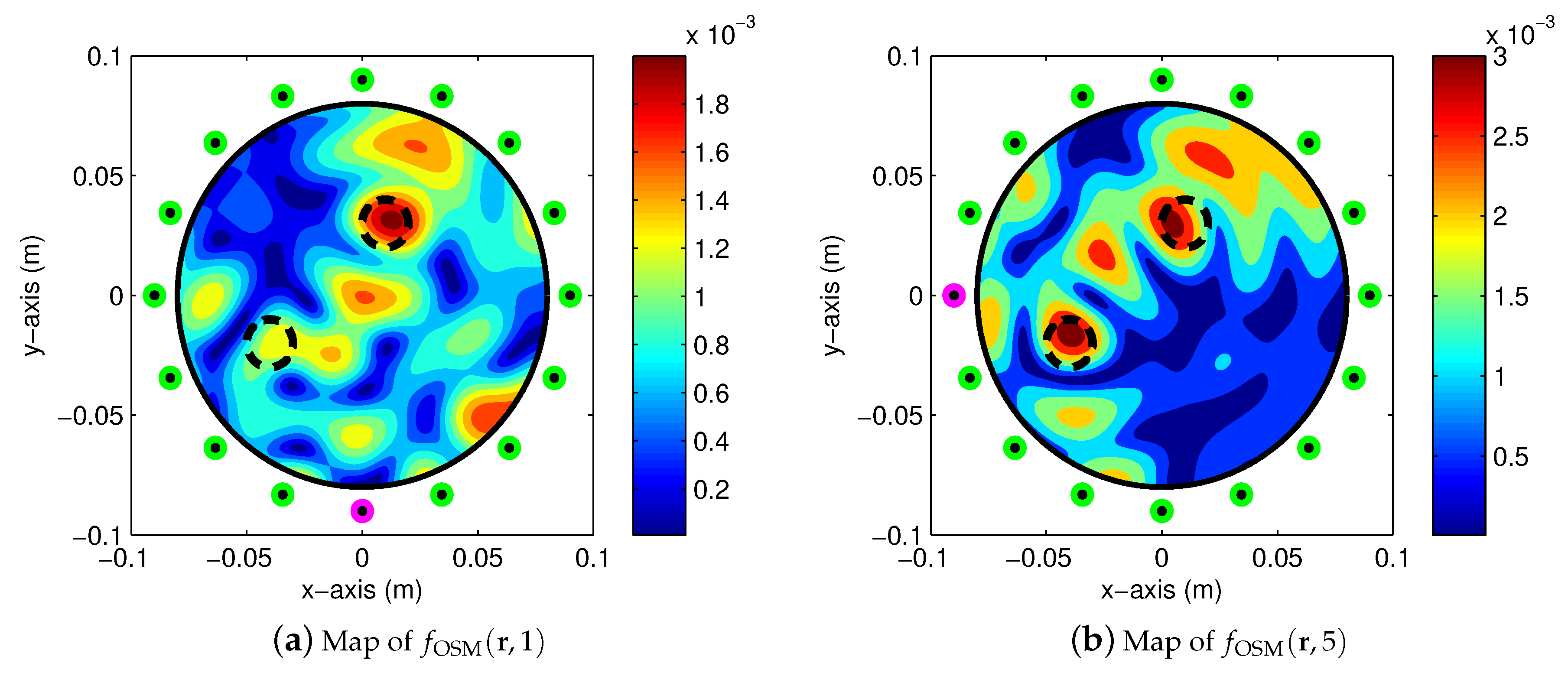
(Localization of multiple anomalies with the same material properties). Based on previous studies and Corollary 1, OSM can be applied directly to multiple anomalies. Now, we apply OSM to the localization of multiple small anomalies ${\mathsf{\Sigma }}_l$, $l=1,2$, with the same radii ${\rho }_l=0.01\mathrm{m}$, permittivity ${\epsilon }_{r1}={\epsilon }_{r2}=55$, and conductivity ${\sigma }_l=1.2\mathrm{S}/\mathrm{m}$ at $f=1.2\mathrm{G}\mathrm{Hz}$, but different locations ${\mathbf{r}}_1={[0.01\mathrm{m},0.03\mathrm{m}]}^T$ and ${\mathbf{r}}_2={[-0.04\mathrm{m},-0.02\mathrm{m}]}^T$; see Figure 4a. Figure 5 shows maps of $f_{OSM}(\mathbf{r},m)$ with various values of m. As with the localization of single anomaly, an anomaly whose location is sufficiently close to the transmitter ${\mathbf{d}}_m$ can be recognized even while another anomaly cannot be identified using the map of $f_{OSM}(\mathbf{r},m)$. Moreover, owing to the appearance of several artifacts, identifying all anomalies is very difficult. Following [16], the possible method to overcome this difficulty would be application of multiple incident fields or frequencies.

Example 4

(Localization of multiple anomalies with different material properties). For the final result, consider the application of OSM to the localization of multiple anomalies ${\mathsf{\Sigma }}_l$, $l=1,2$, with the same radii ${\rho }_l=0.01\mathrm{m}$. The material properties of ${\mathsf{\Sigma }}_1$ are the same as those in Example 3, and the location of ${\mathsf{\Sigma }}_2$ is the same as that in Example 3, while the permittivity and conductivity are set to ${\epsilon }_{r2}=45$ and ${\sigma }_2=1.0\mathrm{S}/\mathrm{m}$, respectively (see Figure 4b). Figure 6 shows maps of $f_{OSM}(\mathbf{r},m)$ with various values of m. As with the results in Example 3, it is difficult to identify all of the anomalies using the map of $f_{OSM}(\mathbf{r},m)$. It is interesting to observe that in contrast to the results in Example 3, the locations of two anomalies are identified well through the map of $f_{OSM}(\mathbf{r},5)$ and the location of ${\mathsf{\Sigma }}_1$ was clearly identified using the map of $f_{OSM}(\mathbf{r},1)$. These results reveal that imaging performance depends on the material properties (such as permittivity and conductivity) and supports the accuracy of the identified structure (9).

5. Conclusions

In this paper, we designed and applied OSM to identify the locations of small anomalies from measured scattered field S-parameters. Based on the established structure of the indicator function, we verified that the identification performance of the indicator function of OSM depends strongly on the applied frequency, total number of measurement data, location of the transmitting antenna, and material properties of each anomaly. Simulation results with synthetic data demonstrated the feasibility and limitations of OSM in microwave imaging. Application of OSM to real-world microwave imaging, improvement of the imaging/detecting performance, and development of the corresponding mathematical theory are left to future work. Finally, we considered the application of OSM in the two-dimensional problem. Extension to the three-dimensional problem will be also an interesting research topic; refer to [40,41,42,43,44] for related work.

References

- Chandra, R.; Johansson, A.J.; Gustafsson, M.; Tufvesson, F. A microwave imaging-based technique to localize an in-body RF source for biomedical applications. IEEE Trans. Biomed. Eng. 2015, 62, 1231–1241. [Google Scholar] [CrossRef] [PubMed]
- Shea, J.D.; Kosmas, P.; Veen, B.D.V.; Hagness, S.C. Contrast-enhanced microwave imaging of breast tumors: A computational study using 3-D realistic numerical phantoms. Inverse Probl. 2010, 26, 074009. [Google Scholar] [CrossRef] [PubMed]
- Simonov, N.; Kim, B.R.; Lee, K.-J.; Jeon, S.-I.; Son, S.-H. Advanced fast 3-D electromagnetic solver for microwave tomography imaging. IEEE Trans. Med. Imaging 2017, 36, 2160–2170. [Google Scholar] [CrossRef] [PubMed]
- Delbary, F.; Erhard, K.; Kress, R.; Potthast, R.; Schulz, J. Inverse electromagnetic scattering in a two-layered medium with an application to mine detection. Inverse Probl. 2008, 24, 015002. [Google Scholar] [CrossRef]
- Kim, C.-K.; Lee, J.-S.; Chae, J.-S.; Park, S.-O. A modified stripmap SAR processing for vector velocity compensation using the cross-correlation estimation method. J. Electromagn. Eng. Sci. 2019, 19, 159–165. [Google Scholar] [CrossRef]
- Soldovieri, F.; Solimene, R. Ground penetrating radar subsurface imaging of buried objects. In Radar Technology; Kouemou, G., Ed.; IntechOpen: Rijeka, Croatia, 2010; Chapter 6; pp. 105–126. [Google Scholar]
- Chang, Q.; Peng, T.; Liu, Y. Tomographic damage imaging based on inverse acoustic wave propagation using k-space method with adjoint method. Mech. Syst. Signal Proc. 2018, 109, 379–398. [Google Scholar] [CrossRef]
- Feng, M.Q.; Flaviis, F.D.; Kim, Y.J. Use of microwaves for damage detection of fiber reinforced polymer-wrapped concrete structures. J. Eng. Mech. 2002, 128, 172–183. [Google Scholar] [CrossRef] [Green Version]
- Kim, Y.J.; Jofre, L.; Flaviis, F.D.; Feng, M.Q. Microwave reflection tomographic array for damage detection of civil structures. IEEE Trans. Antennas Propag. 2003, 51, 3022–3032. [Google Scholar]
- Ammari, H. Mathematical Modeling in Biomedical Imaging II: Optical, Ultrasound, and Opto-Acoustic Tomographies; Lecture Notes in Mathematics; Springer: Berlin/Heidelberg, Germany, 2011; Volume 2035. [Google Scholar]
- Bleistein, N.; Cohen, J.; Stockwell, J.S., Jr. Mathematics of Multidimensional Seismic Imaging, Migration, and Inversion; Springer: New York, NY, USA, 2001. [Google Scholar]
- Colton, D.; Kress, R. Inverse Acoustic and Electromagnetic Scattering Problems; Mathematics and Applications Series; Springer: New York, NY, USA, 1998. [Google Scholar]
- Chandra, R.; Zhou, H.; Balasingham, I.; Narayanan, R.M. On the opportunities and challenges in microwave medical sensing and imaging. IEEE Trans. Biomed. Eng. 2015, 62, 1667–1682. [Google Scholar] [CrossRef] [PubMed]
- Kwon, O.; Seo, J.K.; Yoon, J.R. A real-time algorithm for the location search of discontinuous conductivities with one measurement. Commun. Pur. Appl. Math. 2002, 55, 1–29. [Google Scholar] [CrossRef]
- Park, W.-K.; Lesselier, D. Reconstruction of thin electromagnetic inclusions by a level set method. Inverse Probl. 2009, 25, 085010. [Google Scholar] [CrossRef]
- Potthast, R. A study on orthogonality sampling. Inverse Probl. 2010, 26, 074015. [Google Scholar] [CrossRef]
- Griesmaier, R. Multi-frequency orthogonality sampling for inverse obstacle scattering problems. Inverse Probl. 2011, 27, 085005. [Google Scholar] [CrossRef]
- Akinci, M.N.; Çayören, M.; Akduman, İ. Near-field orthogonality sampling method for microwave imaging: Theory and experimental verification. IEEE Trans. Microw. Theory Tech. 2016, 64, 2489–2501. [Google Scholar] [CrossRef]
- Akinci, M.N. Improving near-field orthogonality sampling method for qualitative microwave imaging. IEEE Trans. Antennas Propag. 2018, 66, 5475–5484. [Google Scholar] [CrossRef]
- Harris, I.; Nguyen, D.L. Orthogonality sampling method for the electromagnetic inverse scattering problem. SIAM J. Sci. Comput. 2020, 42, B722–B737. [Google Scholar] [CrossRef]
- Ahn, C.Y.; Chae, S.; Park, W.-K. Fast identification of short, sound-soft open arcs by the orthogonality sampling method in the limited-aperture inverse scattering problem. Appl. Math. Lett. 2020, 109, 106556. [Google Scholar] [CrossRef]
- Bevacqua, M.T.; Isernia, T.; Palmeri, R.; Akinci, M.N.; Crocco, L. Physical insight unveils new imaging capabilities of orthogonality sampling method. IEEE Trans. Antennas Propag. 2020, 68, 4014–4021. [Google Scholar] [CrossRef]
- Akinci, M.N. An efficient sampling method for cross-borehole GPR imaging. IEEE Geosci. Remote Sens. Lett. 2018, 15, 1857–1861. [Google Scholar] [CrossRef]
- Park, W.-K.; Kim, H.P.; Lee, K.-J.; Son, S.-H. MUSIC algorithm for location searching of dielectric anomalies from S-parameters using microwave imaging. J. Comput. Phys. 2017, 348, 259–270. [Google Scholar] [CrossRef]
- Park, W.-K. Fast location search of small anomaly by using microwave. Int. J. Appl. Electromagn. Mech. 2019, 59, 1505–1510. [Google Scholar] [CrossRef]
- Lee, K.-J.; Son, S.-H.; Park, W.-K. A real-time microwave imaging of unknown anomaly with and without diagonal elements of scattering matrix. Results Phys. 2020, 17, 103104. [Google Scholar] [CrossRef]
- Park, W.-K. Direct sampling method for anomaly imaging from scattering parameter. Appl. Math. Lett. 2018, 81, 63–71. [Google Scholar] [CrossRef] [Green Version]
- Park, W.-K. Real-time microwave imaging of unknown anomalies via scattering matrix. Mech. Syst. Signal Proc. 2019, 118, 658–674. [Google Scholar] [CrossRef] [Green Version]
- Son, S.-H.; Lee, K.-J.; Park, W.-K. Application and analysis of direct sampling method in real-world microwave imaging. Appl. Math. Lett. 2019, 96, 47–53. [Google Scholar] [CrossRef] [Green Version]
- Park, W.-K. Experimental validation of the factorization method to microwave imaging. Results Phys. 2020, 17, 103071. [Google Scholar] [CrossRef]
- Haynes, M.; Stang, J.; Moghaddam, M. Real-time microwave imaging of differential temperature for thermal therapy monitoring. IEEE Trans. Biomed. Eng. 2014, 61, 1787–1797. [Google Scholar] [CrossRef] [PubMed] [Green Version]
- Slaney, M.; Kak, A.C.; Larsen, L.E. Limitations of imaging with first-order diffraction tomography. IEEE Trans. Microw. Theory Tech. 1984, 32, 860–874. [Google Scholar] [CrossRef] [Green Version]
- Fouda, A.E.; Teixeira, F.L. Statistical stability of ultrawideband time-reversal imaging in random media. IEEE Trans. Geosci. Remote Sens. 2014, 52, 870–879. [Google Scholar] [CrossRef]
- Labyed, Y.; Huang, L. Detecting small targets using windowed time-reversal MUSIC imaging: A phantom study. In Proceedings of the 2011 IEEE International Ultrasonics Symposium, Orlando, FL, USA, 18–21 October 2011; pp. 1579–1582. [Google Scholar]
- Marengo, E.A.; Gruber, F.K.; Simonetti, F. Time-reversal MUSIC imaging of extended targets. IEEE Trans. Image Process. 2007, 16, 1967–1984. [Google Scholar] [CrossRef]
- Park, W.-K. Asymptotic properties of MUSIC-type imaging in two-dimensional inverse scattering from thin electromagnetic inclusions. SIAM J. Appl. Math. 2015, 75, 209–228. [Google Scholar] [CrossRef] [Green Version]
- Park, W.-K. Multi-frequency subspace migration for imaging of perfectly conducting, arc-like cracks in full- and limited-view inverse scattering problems. J. Comput. Phys. 2015, 283, 52–80. [Google Scholar] [CrossRef] [Green Version]
- Son, S.-H.; Simonov, N.; Kim, H.J.; Lee, J.M.; Jeon, S.-I. Preclinical prototype development of a microwave tomography system for breast cancer detection. ETRI J. 2010, 32, 901–910. [Google Scholar] [CrossRef]
- Kress, R. Inverse scattering from an open arc. Math. Meth. Appl. Sci. 1995, 18, 267–293. [Google Scholar] [CrossRef]
- Ammari, H.; Iakovleva, E.; Lesselier, D.; Perrusson, G. MUSIC type electromagnetic imaging of a collection of small three-dimensional inclusions. SIAM J. Sci. Comput. 2007, 29, 674–709. [Google Scholar] [CrossRef] [Green Version]
- Iakovleva, E.; Gdoura, S.; Lesselier, D.; Perrusson, G. Multi-static response matrix of a 3D inclusion in half space and MUSIC imaging. IEEE Trans. Antennas Propag. 2007, 55, 2598–2609. [Google Scholar] [CrossRef]
- Liu, K. A simple method for detecting scatterers in a stratified ocean waveguide. Comput. Math. Appl. 2018, 76, 1791–1802. [Google Scholar] [CrossRef]
- Liu, K.; Xu, Y.; Zou, J. A multilevel sampling method for detecting sources in a stratified ocean waveguide. J. Comput. Appl. Math. 2017, 309, 95–110. [Google Scholar] [CrossRef] [Green Version]
- Song, R.; Chen, R.; Chen, X. Imaging three-dimensional anisotropic scatterers in multi-layered medium by MUSIC method with enhanced resolution. J. Opt. Soc. Am. A 2012, 29, 1900–1905. [Google Scholar] [CrossRef]
Figure 1.
Illustration of simulation configuration.
Figure 2.
(Example 1) Maps of . The black-colored dashed circle describes the anomaly boundary.
Figure 3.
(Example 2) Maps of . The black-colored dashed circle describes the anomaly boundary.
Figure 4.
Illustration of simulation configuration for multiple anomalies.
Figure 5.
(Example 3) Maps of . Black-colored dashed circles describe the boundary of anomalies.
Figure 6.
(Example 4) Maps of . Black-colored dashed circles describe the boundary of anomalies.
© 2020 by the authors. Licensee MDPI, Basel, Switzerland. This article is an open access article distributed under the terms and conditions of the Creative Commons Attribution (CC BY) license (http://creativecommons.org/licenses/by/4.0/).
Share and Cite
MDPI and ACS Style
Chae, S.; Ahn, C.Y.; Park, W.-K. Localization of Small Anomalies via the Orthogonality Sampling Method from Scattering Parameters. Electronics 2020, 9, 1119. https://0-doi-org.brum.beds.ac.uk/10.3390/electronics9071119
AMA Style
Chae S, Ahn CY, Park W-K. Localization of Small Anomalies via the Orthogonality Sampling Method from Scattering Parameters. Electronics. 2020; 9(7):1119. https://0-doi-org.brum.beds.ac.uk/10.3390/electronics9071119
Chicago/Turabian StyleChae, Seongje, Chi Young Ahn, and Won-Kwang Park. 2020. "Localization of Small Anomalies via the Orthogonality Sampling Method from Scattering Parameters" Electronics 9, no. 7: 1119. https://0-doi-org.brum.beds.ac.uk/10.3390/electronics9071119
Note that from the first issue of 2016, this journal uses article numbers instead of page numbers. See further details here.