1. Introduction
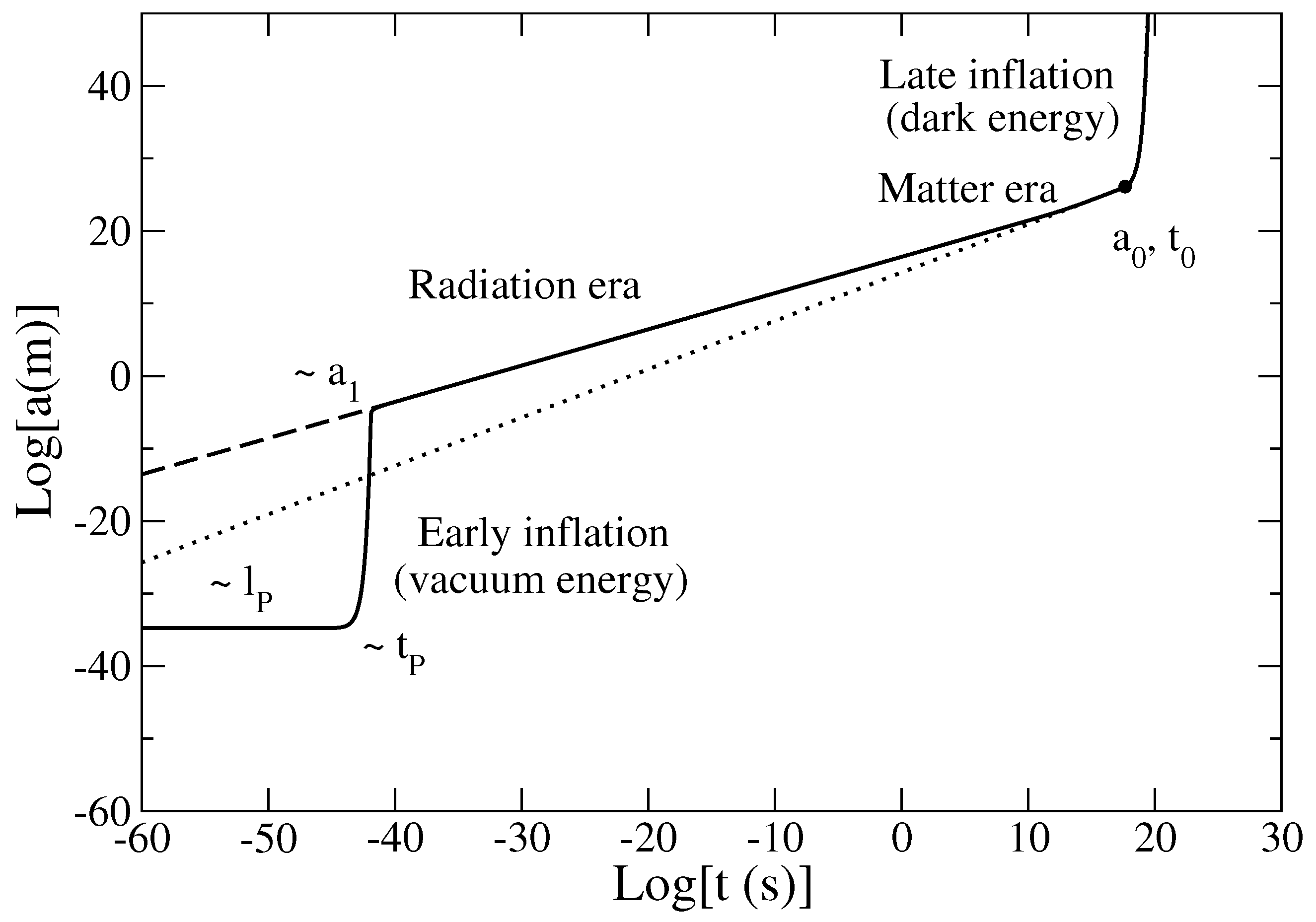
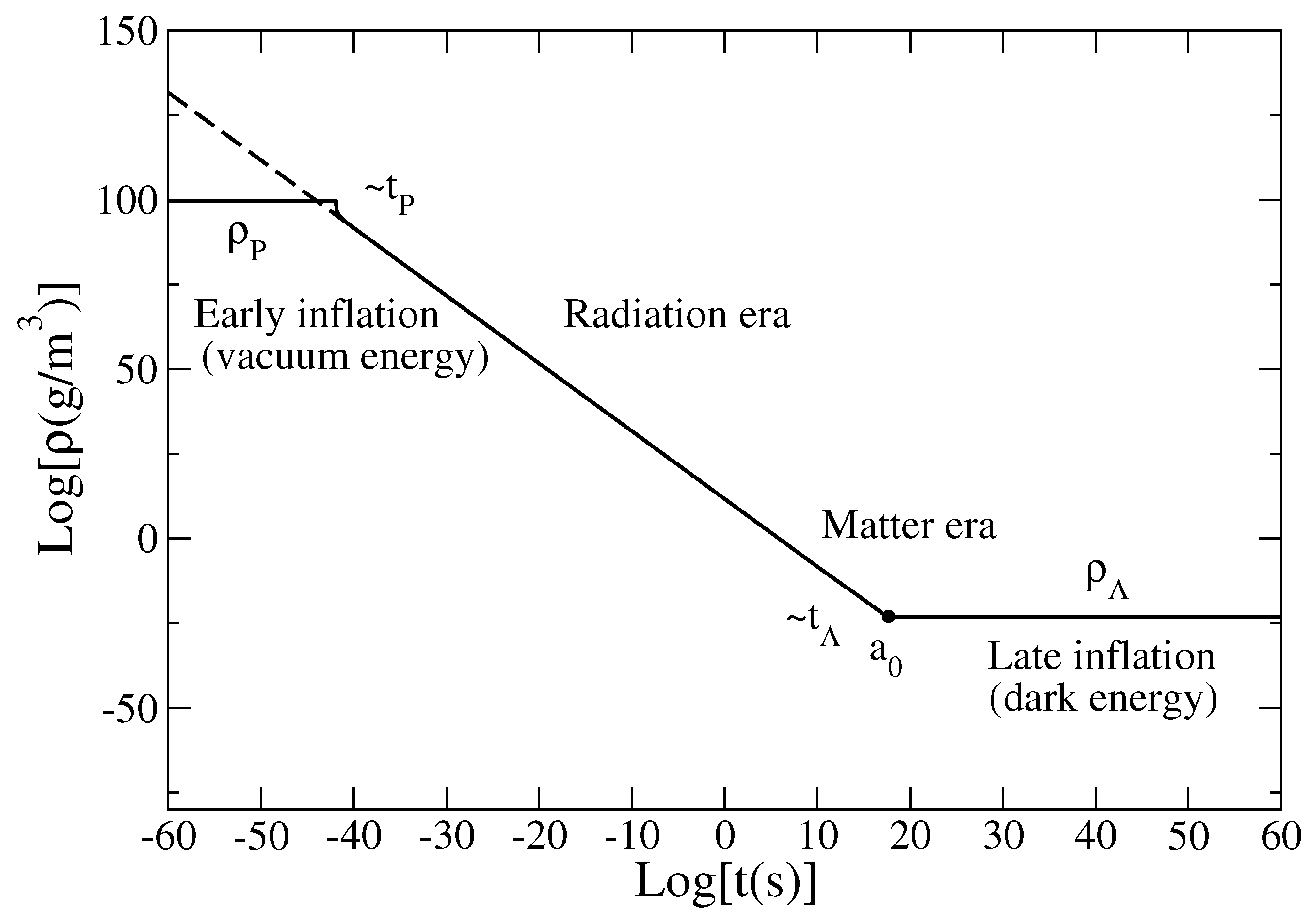
The evolution of the universe may be divided into four main periods [
1]. In the vacuum energy era (Planck era), the universe undergoes a phase of early inflation that brings it from the Planck size
to an almost “macroscopic” size
in a tiniest fraction of a second [
2,
3,
4,
5]. The universe then enters in the radiation era and, when the temperature cools down below approximately
, in the matter era [
6]. Finally, in the dark energy era (de Sitter era), the universe undergoes a phase of late inflation [
7]. The early inflation is necessary to solve notorious difficulties such as the singularity problem, the flatness problem, and the horizon problem [
2,
3,
4,
5]. The late inflation is necessary to account for the observed accelerating expansion of the universe [
8,
9,
10,
11]. At present, the universe is composed of approximately
baryonic matter,
dark matter, and
dark energy [
1]. Despite the success of the standard ΛCDM model, the nature of vacuum energy, dark matter, and dark energy remains very mysterious and leads to many speculations.
The phase of inflation in the early universe is usually described by some hypothetical scalar field
ϕ, called inflaton, with its origin in the quantum fluctuations of the vacuum [
2,
3,
4,
5]. This leads to an equation of state
, implying a constant energy density, called the vacuum energy. This energy density is usually identified with the Planck density
. As a result of the vacuum energy, the universe expands exponentially rapidly on a timescale of the order of the Planck time
.
The phase of acceleration in the late universe is usually ascribed to the cosmological constant Λ which is equivalent to a constant energy density
called the dark energy [
7]. This acceleration can be modeled by an equation of state
implying a constant energy density identified with the cosmological density
. As a result of the dark energy, the universe expands exponentially rapidly on a timescale of the order of the cosmological time
(de Sitter solution). This leads to a phase of late inflation. Instead of introducing a cosmological constant, some authors have proposed to explain the acceleration of the universe in terms of a dark energy with a time-varying density associated with a canonical scalar field called quintessence [
12,
13,
14,
15,
16,
17,
18,
19,
20,
21,
22,
23,
24], or in terms of a tachyonic field [
25,
26,
27,
28].
Between the phase of early inflation and the phase of late accelerating expansion, the universe is in the radiation era, then in the matter era [
6]. These phases are described by a linear equation of state
with
for the radiation and
for the pressureless matter (including baryonic matter and dark matter). The scale factor increases algebraically as
and the density decreases algebraically as
. For
, the universe is decelerating.
In recent works [
29,
30,
31,
32], we have proposed to describe the transition between a phase of algebraic expansion (
) and a phase of exponential expansion (
) by a generalized polytropic equation of state of the form
This is the sum of a standard linear equation of state
and a polytropic equation of state
with
. Polytropic equations of state play an important role in astrophysics [
33,
34], statistical physics [
35] and mathematical biology [
36], and they may also be relevant in cosmology. We have studied the equation of state (
1) for any values of
α,
k and
n and found the following structure. Positive indices
describe the early universe where the polytropic component dominates the linear component because the density is high. Negative indices
describe the late universe where the polytropic component dominates the linear component because the density is low. On the other hand, a positive polytropic pressure (
) leads to past or future singularities (or peculiarities) while a negative polytropic pressure (
) leads to a phase of exponential expansion (inflation) in the past or in the future [Note 1: the polytropic equation of state (
1) with
and
is equivalent to the generalized Chaplygin gas model
with
that has been proposed to describe the late accelerating expansion of the universe (the original Chaplygin gas model corresponds to
and
) [
37,
38,
39,
40,
41,
42,
43,
44,
45]. Therefore, the polytropic equation of state (
1) with
and
introduced in [
29] can be seen as an extension of the generalized Chaplygin gas model to describe the early accelerating expansion of the universe (inflation).]. In the early universe (
,
), the generalized polytropic equation of state (
1) leads to a maximum bound for the density that it is natural to identify with the Planck density
(vacuum energy). In the late universe (
,
), it leads to a minimum bound for the density that it is natural to identify with the cosmological density
(dark energy). These bounds differ by 122 orders of magnitude. Taking
,
and
we obtain an equation of state
that describes the transition between the vacuum energy era (
) and the radiation era. On the other hand, taking
,
and
we obtain an equation of state
that describes the transition between the matter era and the dark energy era (
). More generally, the equation of state
describes the transition between the vacuum energy era and an
α-era in the early universe, and the equation of state
describes the transition between an
α-era and the dark energy era in the late universe.
In this paper, we propose to describe the vacuum energy, the
α-fluid, and the dark energy in a “unified” manner by a single, quadratic, equation of state of the form [Note 2: This idea was sketched in [
30,
32] and is here systematically developed.]:
involving the Planck density and the cosmological density [Note 3: It is oftentimes argued that the dark energy (cosmological constant) corresponds to the vacuum energy. This leads to the so-called
cosmological constant problem [
46,
47] because the cosmological density
and the Planck density
differ by about 122 orders of magnitude. We think it is a mistake to identify the dark energy with the vacuum energy. In this paper, we regard the vacuum energy and the dark energy as two distinct entities. We call vacuum energy the energy associated with the Planck density and dark energy the energy associated with the cosmological density. The vacuum energy is responsible for the inflation of the early universe and the dark energy for the inflation (acceleration) of the late universe. In this viewpoint, the vacuum energy is due to quantum mechanics and the dark energy is an effect of general relativity. The cosmological constant Λ is interpreted as a fundamental constant of nature applying to the cosmophysics in the same way the Planck constant ℏ applies to the microphysics.]. In the early universe (
), we recover the equation of state
unifying the vacuum energy (
) and the
α-fluid. In the late universe (
), we recover the equation of state
unifying the
α-fluid and the dark energy (
). The
α-fluid may represent radiation (
) or pressureless dark matter (
). Actually, some works [
48] indicate that dark matter may be described by an isothermal equation of state
with a small value of
. It is therefore useful to leave
α unspecified and treat the general case of arbitrary
α. However, to simplify the discussion, we shall assume
. Moreover, for illustrations, we will select the values
(radiation) and
(pressureless matter) considered in our previous studies [
29,
30,
31,
32].
The quadratic equation of state (
2) leads to a fully analytical cosmological model describing the evolution of the universe from the initial inflation (Planck era) to the late accelerating expansion (de Sitter era). These two phases are bridged by an algebraic decelerating expansion (
α-era). The pressure is successively negative (vacuum energy), positive (
α-era), and negative again (dark energy). Our model does not present any singularity at
—the phase of early inflation avoids the primordial Big Bang singularity—and exists eternally in the past (although it may be incorrect to extrapolate the solution to the infinite past). On the other hand, our model admits a scalar field interpretation based on an inflaton, quintessence, or tachyonic field. This correspondence is interesting because the early inflation and the late acceleration of the universe are usually described in terms of a scalar field. There exist general techniques [
7,
49] to represent a fluid model in terms of a (canonical or tachyonic) scalar field. Although the hydrodynamic and field representations are equivalent at the background level, they may totally differ at the level of the perturbations when the fluid has a negative pressure. As a result, it is important to give the two representations and study the evolution of the perturbations in each case. It is known that the scalar field representation is more complete than the hydrodynamic representation, and provides a more realistic model [Note 4: The perfect fluid approach is more rough than the scalar field approach because for given perfect fluid variables
ρ and
P one cannot restore the scalar field variables
ϕ,
and
in the inhomogeneous case (while the converse is always possible).]. In this paper, we only consider the evolution of the background where the hydrodynamic and field representations are equivalent. The study of the perturbations will be considered in future works.
The paper is organized as follows. In
Section 2, we recall the basic equations of cosmology that are needed in our study. In
Section 3, we describe the transition between the vacuum energy era (
) and the
α-era in the early universe. In
Section 4, we describe the transition between the
α-era and the dark energy era (
) in the late universe. In
Section 5, we introduce the general model where vacuum energy +
α-era + dark energy are described by the quadratic equation of state (
2). This model reveals a nice “symmetry” between the early universe (vacuum energy +
α-era) and the late universe (
α-era + dark energy). These two phases are described by two polytropic equations of state with index
and
respectively. The mathematical formulae in the early and in the late universe are strikingly symmetric. Furthermore, the cosmological density
in the late universe plays a role similar to the Planck density
in the early universe. They represent fundamental lower and upper density bounds differing by 122 orders of magnitude. Interestingly, these densities
and
(together with
α) appear as the coefficients of the equation of state (
2). Therefore, this equation of state provides a “unification” of vacuum energy and dark energy. We propose to interpret vacuum energy, radiation and dark energy as a “generalized radiation” described by the equation of state (
2) with
and treat baryonic matter and dark matter as independent species. This leads to Equation (
110) that generalizes Equation (
107) of the standard ΛCDM model. This equation avoids the primordial singularity and describes the whole evolution of the universe from the early inflation to the late accelerating expansion. In
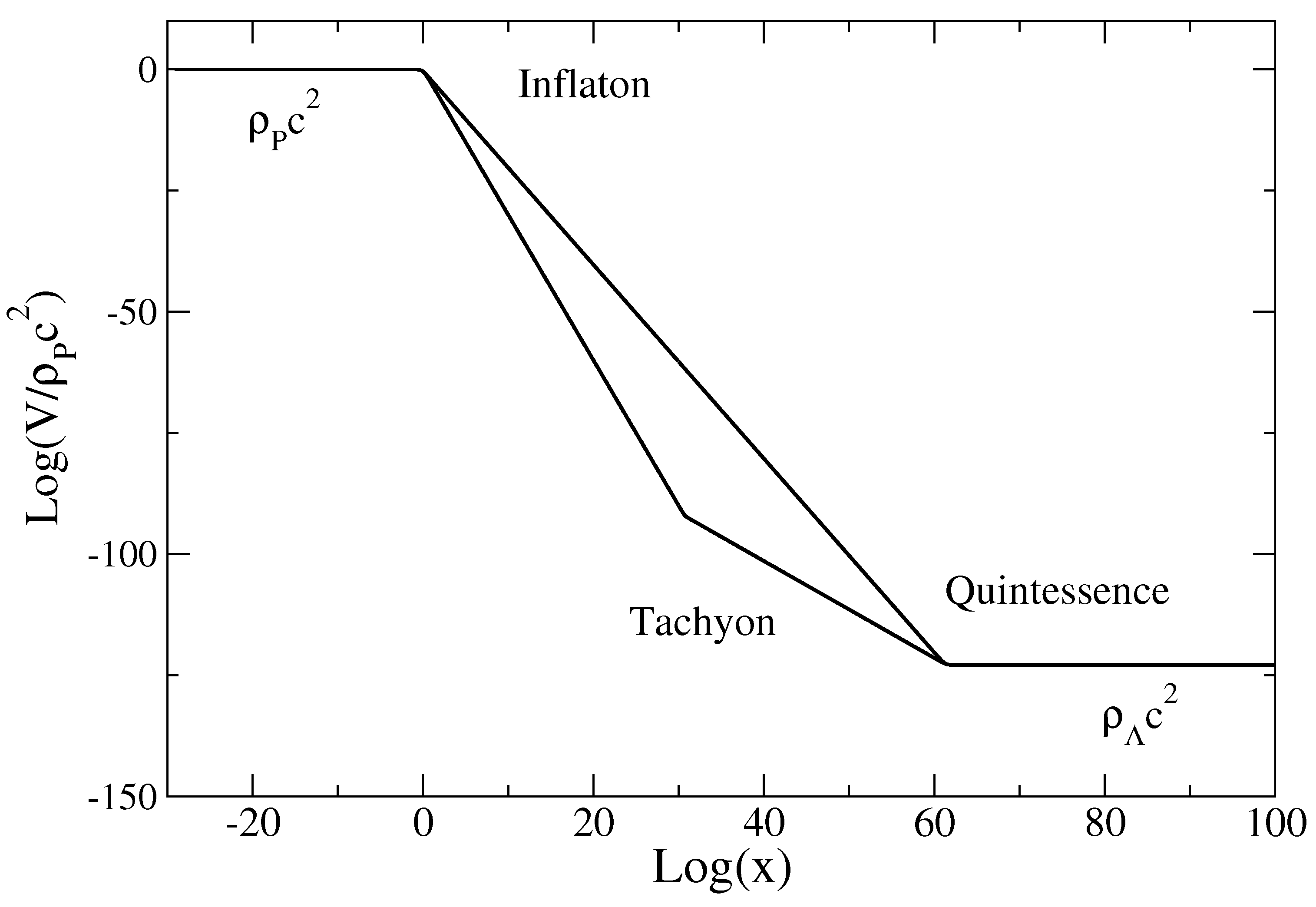
Appendix A, we develop a scalar field theory and derive the potential
associated with the quadratic equation of state (
2). This potential (see Equations (
119)–(
121)) unifies the inflaton potential in the early universe (see Equation (
35)) and the quintessence potential in the late universe (see Equation (
62)).
2. Basic Equations of Cosmology
In a space with uniform curvature, the line element of the expanding universe is given by the Friedmann-Lemaître-Roberston-Walker (FLRW) metric
where
represents the radius of curvature of the 3-dimensional space, or the scale factor. By an abuse of language, we shall sometimes call it the “radius of the universe”. On the other hand,
k determines the curvature of space. The universe may be closed (
), flat (
), or open (
).
If the universe is isotropic and homogeneous at all points in conformity with the line element of Equation (
3), and contains a uniform perfect fluid of energy density
and isotropic pressure
, the energy-momentum tensor
is
The Einstein equations
relate the geometrical structure of the spacetime (
) to the content of the universe (
). For the sake of generality, we have accounted for a possibly non-zero cosmological constant Λ. Given Equations (
3) and (
4), these equations reduce to
where dots denote differentiation with respect to time. These are the well-known cosmological equations describing a non-static universe first derived by Friedmann [
6].
The Friedmann equations are usually written in the form
where we have introduced the Hubble parameter
. Among these three equations, only two are independent. The first equation, which can be viewed as an “equation of continuity”, can be directly derived from the conservation of the energy momentum tensor
which results from the Bianchi identities. For a given barotropic equation of state
, it determines the relation between the density and the scale factor. Then, the temporal evolution of the scale factor is given by Equation (
9).
In this paper, we consider a flat universe (
) in agreement with the observations of the cosmic microwave background (CMB) [
50,
51]. On the other hand, we set
because the contribution of the dark energy will be taken into account in the equation of state. The Friedmann equations then reduce to
The deceleration parameter is defined by
The universe is decelerating when
and accelerating when
. Introducing the equation of state parameter
, and using the Friedmann equations (
11) and (
12), we obtain for a flat universe
We see from Equations (
11) and (
14) that the universe is decelerating if
(strong energy condition) and accelerating if
[Note 5: According to general relativity, the source for the gravitational potential is
. Indeed, the spatial part
of the geodesic acceleration satisfies the exact equation
showing that the source of geodesic acceleration is
not
ρ [
47]. Therefore, in general relativity, gravitation becomes “repulsive” when
.]. On the other hand, according to Equation (
10), the density decreases with the scale factor if
(null dominant energy condition) and increases with the scale factor if
. The latter case corresponds to a “phantom” universe [
52,
53,
54,
55,
56,
57,
58,
59,
60,
61,
62,
63,
64,
65,
66,
67,
68,
69].
3. The Early Universe
In Reference [
29], we have proposed to describe the transition between the vacuum energy era and the
α-era in the early universe by a single equation of state of the form of Equation (
1) with
and
. It can be written as
Assuming
, the equation of continuity (
10) can be integrated into
where
and
is a constant of integration. We see that
corresponds to an upper bound (maximum value) for the density reached for
. Since this solution describes the early universe, it is natural to identify
with the Planck density
. As a result, the equation of state (
15) can be rewritten as
For the sake of simplicity, and for definiteness, we shall select the index
. The general case
has been treated in [
29] and leads to qualitatively similar results. Therefore, we propose to describe the transition between the vacuum energy era and the
α-era in the early universe by a single equation of state of the form
where
is the Planck density. This equation of state corresponds to a generalized polytropic equation of state (
1) with
and
. For
, we recover the linear equation of state
. For
, we get
corresponding to the vacuum energy. The relation of Equation (
16) between the density and the scale factor becomes
The characteristic scale
marks the transition between the vacuum energy era and the
α-era. The equation of state (
18) interpolates smoothly between the vacuum energy era (
,
) and the
α-era (
,
). It provides therefore a “unified” description of the vacuum energy (Planck) era and
α-era in the early universe. This amounts to summing the
inverse of the densities of these two phases. Indeed, Equation (
19) can be rewritten as
At
we have
so that
. Writing
, where
is the present value of the scale factor and
is the present density of the
α-fluid, and using the asymptotic expression
, we find that the transition scale factor
is determined by the relation
.
The equation of state parameter
and the deceleration parameter
q are given by
The velocity of sound
is given by
As the universe expands from
to
, the density decreases from
to 0, the equation of state parameter
w increases from
to
α, the deceleration parameter
q increases from
to
, and the ratio
increases from
to
α (see Figures 2 and 6 of [
29]).
3.1. The Vacuum Energy Era: Early Inflation
When
, the density tends to a maximum value
and the pressure tends to
. The Planck density
(vacuum energy) represents a fundamental upper bound for the density. A constant value of the density
gives rise to a phase of early inflation. From the Friedmann equation (
12), we find that the Hubble parameter is constant,
, where we have introduced the Planck time
. Numerically,
. Therefore, for
, the scale factor increases exponentially rapidly with time as
The timescale of the exponential growth is the Planck time
. We have defined the “original” time
such that
is equal to the Planck length
. Mathematically speaking, the universe exists at any time in the past (
and
for
), so there is no primordial singularity (Big Bang). However, when
, we cannot ignore the quantum fluctuations associated with the spacetime. In that case, we cannot use the classical Einstein equations anymore and a theory of quantum gravity is required. It is not known whether quantum gravity will remove, or not, the primordial singularity. Therefore, we cannot extrapolate the solution in Equation (
24) to the infinite past. However, this solution may provide a
semi-classical description of the phase of early inflation when
.
3.2. The α-Era
When
, we recover the equation
corresponding to the pure linear equation of state
. When
, the Friedmann equation (
12) yields
We then have
During the
α-era, the scale factor increases algebraically as
and the density decreases algebraically as
.
3.3. The General Solution
For the equation of state (
18), the density is related to the scale factor by Equation (
19). It is possible to solve the Friedmann equation (
12) with the density-radius relation of Equation (
19) analytically. Introducing
, we obtain
which can be integrated into [
29]:
where
C is a constant of integration determined such that
at
. Setting
, we get
For
, Equation (
29) reduces to Equation (
26). For
, we have the exact asymptotic result
with
. In general
(for the radiation
, we find
[
29]), so that
C and
D can be approximated by
and
. With this approximation, Equation (
31) returns Equation (
24). The time
marking the end of the inflation is obtained by substituting
in Equation (
29). According to Equation (
21), the universe is accelerating when
(
i.e.,
) and decelerating when
(
i.e.,
) where
and
. The time
at which the universe starts decelerating is obtained by substituting
in Equation (
29). This corresponds to the time at which the curve
presents an inflexion point. For
(radiation) this inflexion point
coincides with
so it also marks the end of the inflation (
). For
the two points differ.
3.4. The Pressure
The pressure is given by Equation (
18). Using Equation (
19), we get
The pressure starts from
at
, remains approximately constant during the inflation, increases at the end of the inflation, becomes positive, reaches a maximum value
, and decreases algebraically during the
α-era. At
,
. The point at which the pressure vanishes (
) corresponds to
and
. On the other hand, the pressure reaches its maximum (
) when
and
[Note 6: The velocity of sound is imaginary (
) when
and real (
) when
. It is always less than the speed of light.]. The maximum pressure is
. At the transition point
, we have
. At the deceleration point
, we have
.
3.5. The Evolution of the Early Universe
In our model, the universe “starts” at
with a vanishing radius
, a finite density
, and a finite pressure
. The universe exists at any time in the past and does not present any singularity. For
, the radius of the universe is less than the Planck length
. In the Planck era, quantum gravity should be taken into account so our semi-classical approach is probably not valid in the infinite past. At
, the radius of the universe is equal to the Planck length
. The corresponding density and pressure are
and
. We note that quantum mechanics regularizes the finite time singularity present in the standard Big Bang theory. This is similar to finite size effects in second order phase transitions (see
Section 3.6). The Big Bang theory is recovered for
. The universe first undergoes a phase of inflation during which its radius increases exponentially rapidly with time while its density and pressure remain approximately constant. The inflation “starts” at
and ends at
. The timescale of the inflation corresponds to the Planck time
(for the radiation
, we find
[
29]). During this very short lapse of time, the scale factor grows from
to
(for
, we find
). By contrast, the density and the pressure do not change significatively: they go from
and
to
and
(for
, we find
and
). The pressure passes from negative values to positive values at
(for
, we find
,
,
). After the inflation, the universe enters in the
α-era. The radius increases algebraically as
while the density decreases algebraically as
. The pressure achieves its maximum value
at
(for
, we find
,
,
,
). During the inflation, the universe is accelerating and during the
α-era it is decelerating (if
). The transition (marked by an inflexion point) takes place at a time
(for
it coincides with the end of the inflation
). The evolution of the scale factor and density as a function of time are represented in
Figure 1,
Figure 2,
Figure 3,
Figure 4 and
Figure 5 in logarithmic and linear scales (the figures correspond to the radiation
).
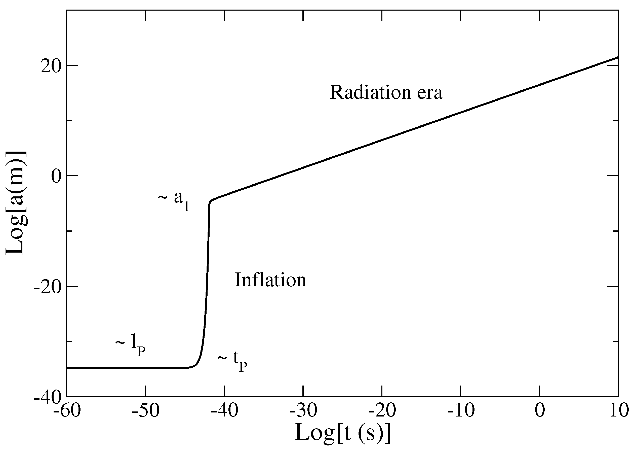
Figure 1.
Evolution of the scale factor a with the time t in logarithmic scales. This figure clearly shows the phase of inflation connecting the vacuum energy era to the α-era (representing here the radiation era). During the inflation, the scale factor increases exponentially rapidly on a timescale of the order of the Planck time (for it increases by 29 orders of magnitude in less than s). In the α-era, the scale factor increases algebraically as .
Figure 2.
Evolution of the scale factor
a with the time
t in linear scales. The dashed line corresponds to a pure linear equation of state
leading to a finite time singularity at
where
(Big Bang). When quantum mechanics is taken into account (as in our semi-classical model), the initial singularity is smoothed-out and the scale factor at
is equal to the Planck length
. This is similar to a second order phase transition where the Planck constant plays the role of finite size effects (see
Section 3.6 for a development of this analogy).
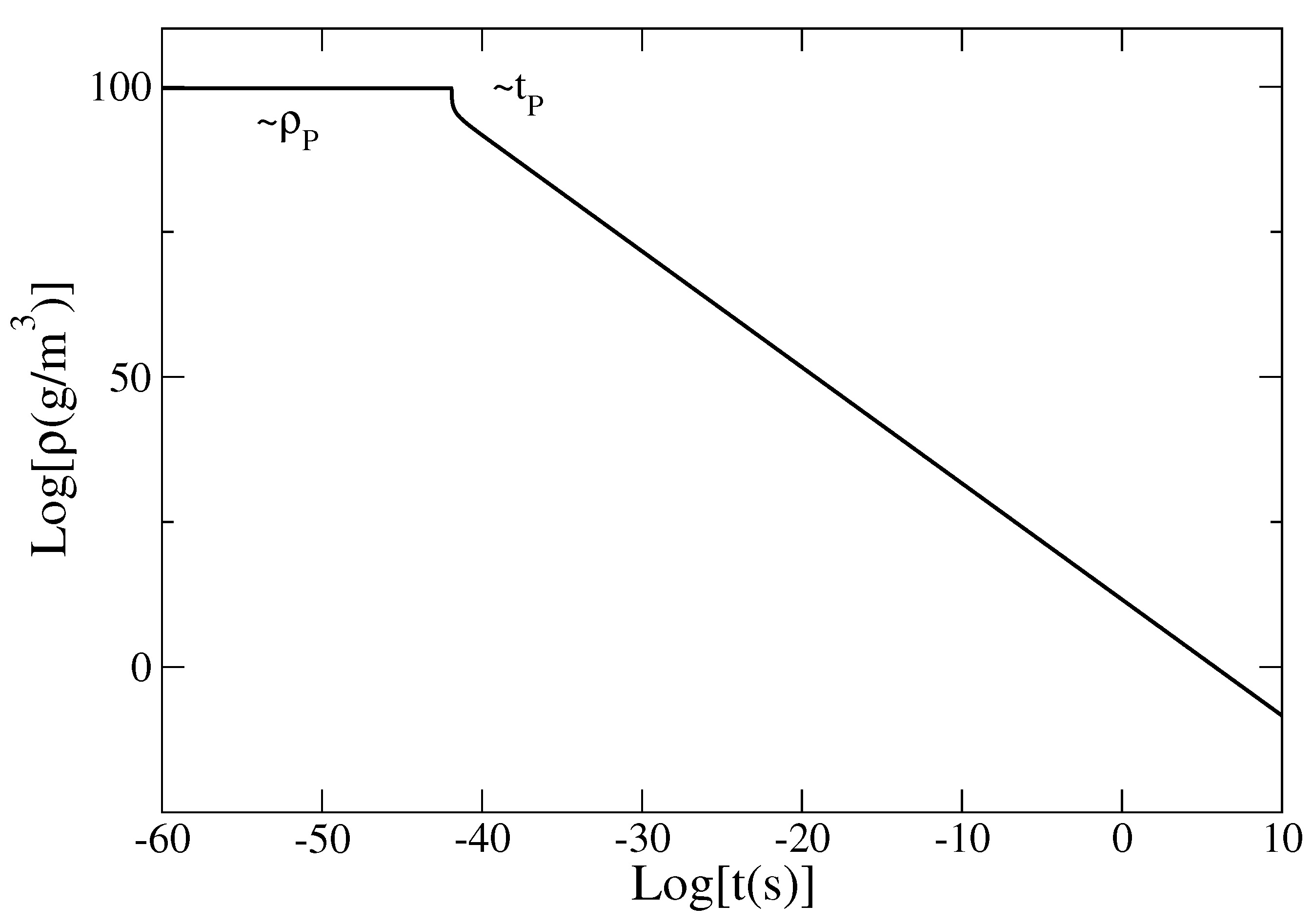
Figure 3.
Evolution of the density ρ with the time t in logarithmic scales. During the inflation, the density remains approximately constant with the Planck value which represents an upper bound. In the α-era, ρ decreases algebraically as .
Figure 3.
Evolution of the density ρ with the time t in logarithmic scales. During the inflation, the density remains approximately constant with the Planck value which represents an upper bound. In the α-era, ρ decreases algebraically as .
Figure 4.
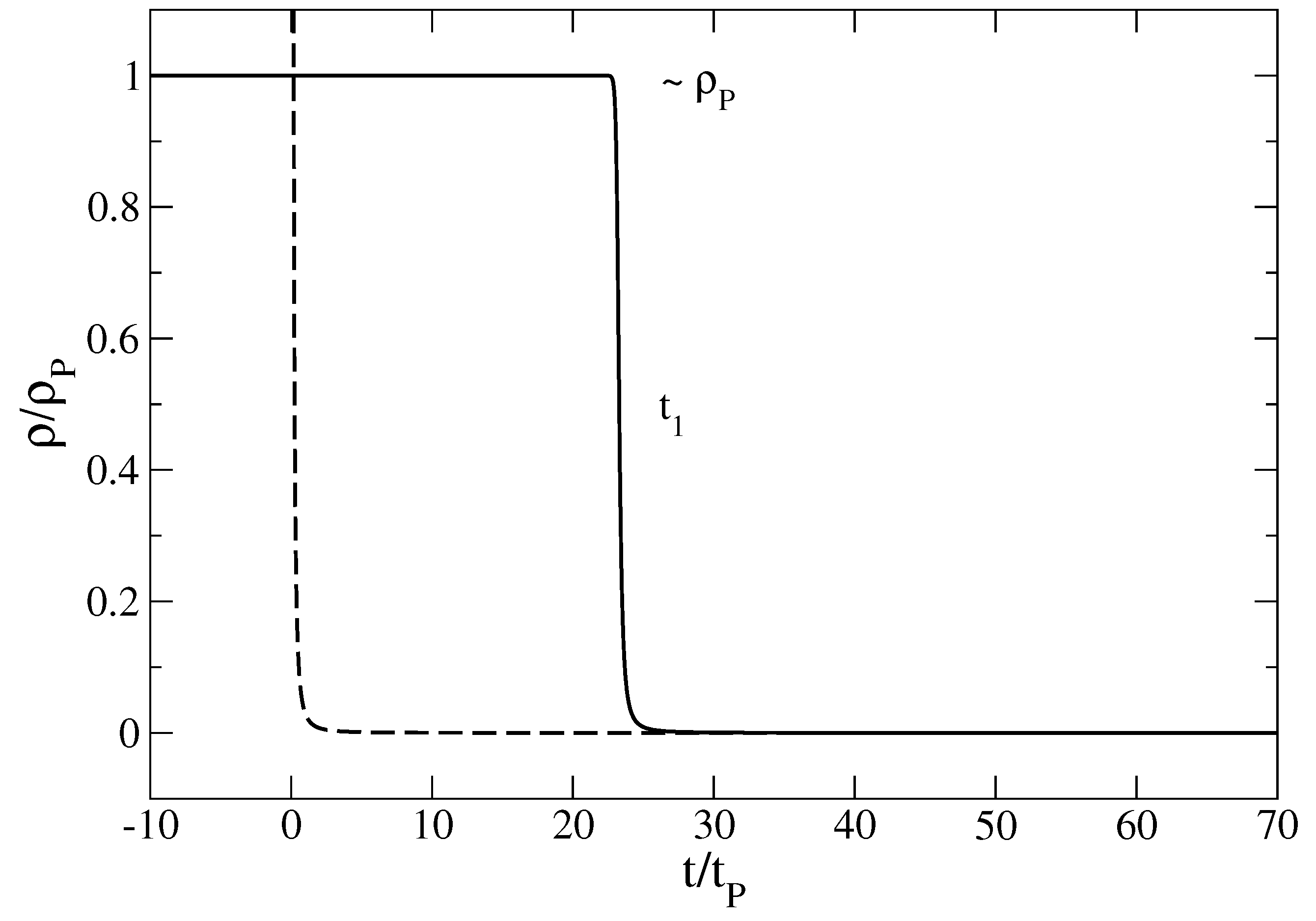
Evolution of the density ρ with the time t in linear scales. The dashed line corresponds to a pure linear equation of state leading to a finite time singularity at . Quantum mechanics limits the rise of the density to the Planck value .
Figure 4.
Evolution of the density ρ with the time t in linear scales. The dashed line corresponds to a pure linear equation of state leading to a finite time singularity at . Quantum mechanics limits the rise of the density to the Planck value .
Remark: If we consider the transition between the inflation era and the radiation era (
), we find that the temperature is given by a generalized Stefan-Boltzmann law (see Equation (84a) in [
29]). The evolution of the temperature is discussed in detail in References [
29,
32,
70]. In our model, the temperature is initially very low, increases exponentially rapidly during the inflation up to a fraction (
) of the Planck temperature
which is of the order of the Grand Unified Theories (GUT) scale, then decreases algebraically during the radiation era. On the other hand, our model generates a value of the entropy as large as
[
29]. This is very different from the standard inflationary scenario [
2,
3,
4,
5]. In that scenario, the universe is radiation dominated up to
and expands exponentially rapidly by a factor
in the interval
with
. For
, the evolution is again radiation dominated. At
, the temperature is about
(this corresponds to the epoch at which most GUTs have a significant influence on the evolution of the universe). During the exponential inflation, the temperature drops drastically and one must advocate a phase of re-heating by various high energy processes (not very well understood) to restore the initial temperature.
Figure 5.
Evolution of the pressure p with the time t in linear scales. The dashed line corresponds to a pure linear equation of state leading to a finite time singularity at . Quantum mechanics limits the rise of the pressure to a maximum value . In the vacuum energy era, the pressure decreases exponentially rapidly as we go backward in time, becomes negative, and tends to for .
3.6. Analogy with Phase Transitions
The standard Big Bang theory is a classical theory in which quantum effects are neglected. In that case, it exhibits a finite time singularity: the radius of the universe is equal to zero at while its density is infinite. For , the solution is not defined and we may take . For the radius of the universe increases as . This is similar to a second order phase transition if we view the time t as the control parameter (e.g., the temperature T) and the scale factor a as the order parameter (e.g., the magnetization M). For (radiation), it is amusing to note that the exponent in is the same as in mean field theories of second order phase transitions (i.e., ) but this is essentially a coincidence.
When quantum mechanics is taken into account, as in our semi-classical model, the singularity at
disappears and the curves
and
are regularized. In particular, we find that
at
, instead of
, due to the finite value of ℏ. This is similar to the regularization due to finite size effects (e.g., the system size
L or the number of particles
N) in ordinary phase transitions. In this sense, the classical limit
is similar to the thermodynamic limit (
or
) in ordinary phase transitions. The convergence of our semi-classical solution towards the classical Big Bang solution when
is shown in
Figure 6 for
(radiation).
Figure 6.
Effect of quantum mechanics (finite value of the Planck constant) on the regularization of the singular Big Bang solution (
, dashed line) in our semi-classical model (see [
29] for details about the construction of this curve). The singularity at
is replaced by an inflationary expansion from the vacuum energy era to the
α-era. We can draw an analogy with second order phase transitions where the Planck constant plays the role of finite size effects.
3.7. Scalar field theory
The phase of inflation in the very early universe is usually described by a scalar field called inflaton [
5]. A canonical scalar field minimally coupled to gravity evolves according to the Klein-Gordon equation
where
is the potential of the scalar field. The scalar field tends to run down the potential towards lower energies. The density and the pressure of the universe are related to the scalar field by
Using standard techniques [
7,
49], we find that the inflaton potential corresponding to the equation of state (
18) is (see Section 8.1 of [
30]):
where we have defined
For
,
which is consistent with the symmetry breaking scalar field potential used to describe inflation. For
,
We can also show [
30] that the relation between the scalar field and the scale factor is
The end of the inflation, and the beginning of the
α-era, corresponds to
, hence to
. Combining Equations (
18), (
19) and (
40), we find that the energy density and the pressure of the universe are related to the scalar field by
Using Equation (
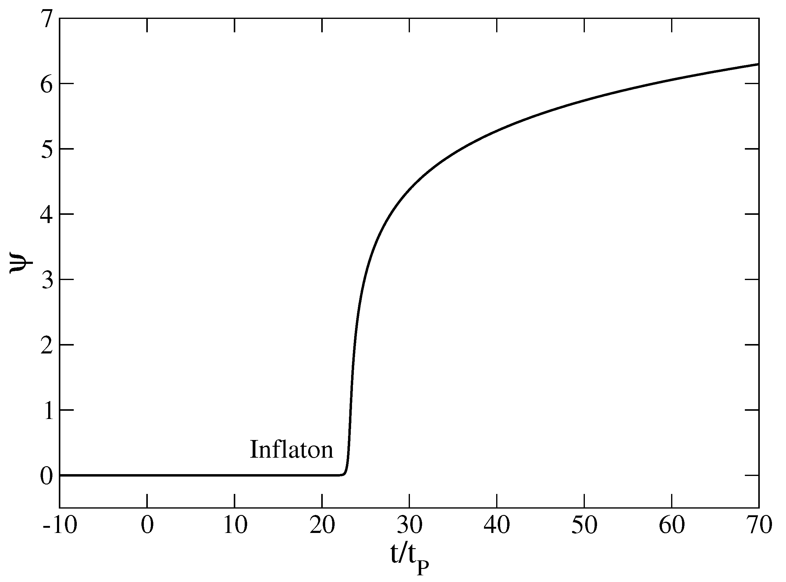
40), and the results of the previous sections, we can obtain the temporal evolution of the scalar field. In the vacuum energy era (
), using Equation (
24), we get
In the
α-era (
), using Equation (
26), we get
More generally, using Equation (
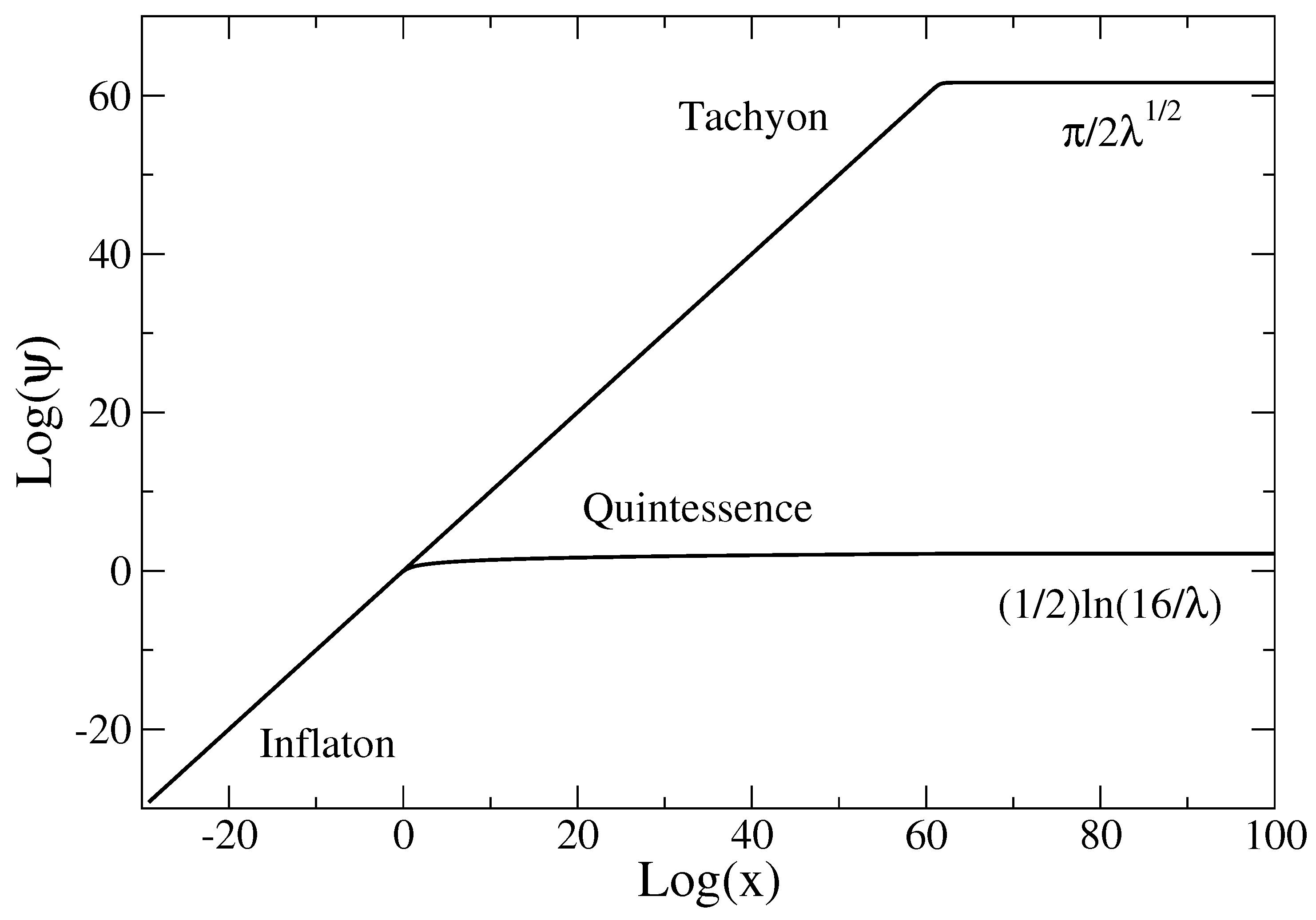
29), the evolution of the scalar field
in the early universe is given by
These results are illustrated in
Figure 7 and
Figure 8 for
(radiation).
Remark: The canonical scalar field potential of Equation (
35) describing the transition between the inflation (vacuum energy) era and the
α-era involves hyperbolic functions. The inflation due to another scalar field with a hyperbolic potential was investigated recently in [
71] and confronted to the Planck 2015 data set, giving promising results. We are carrying out a similar study with the scalar field potential of Equation (
35) to test its performance against Planck inflationary parameters.
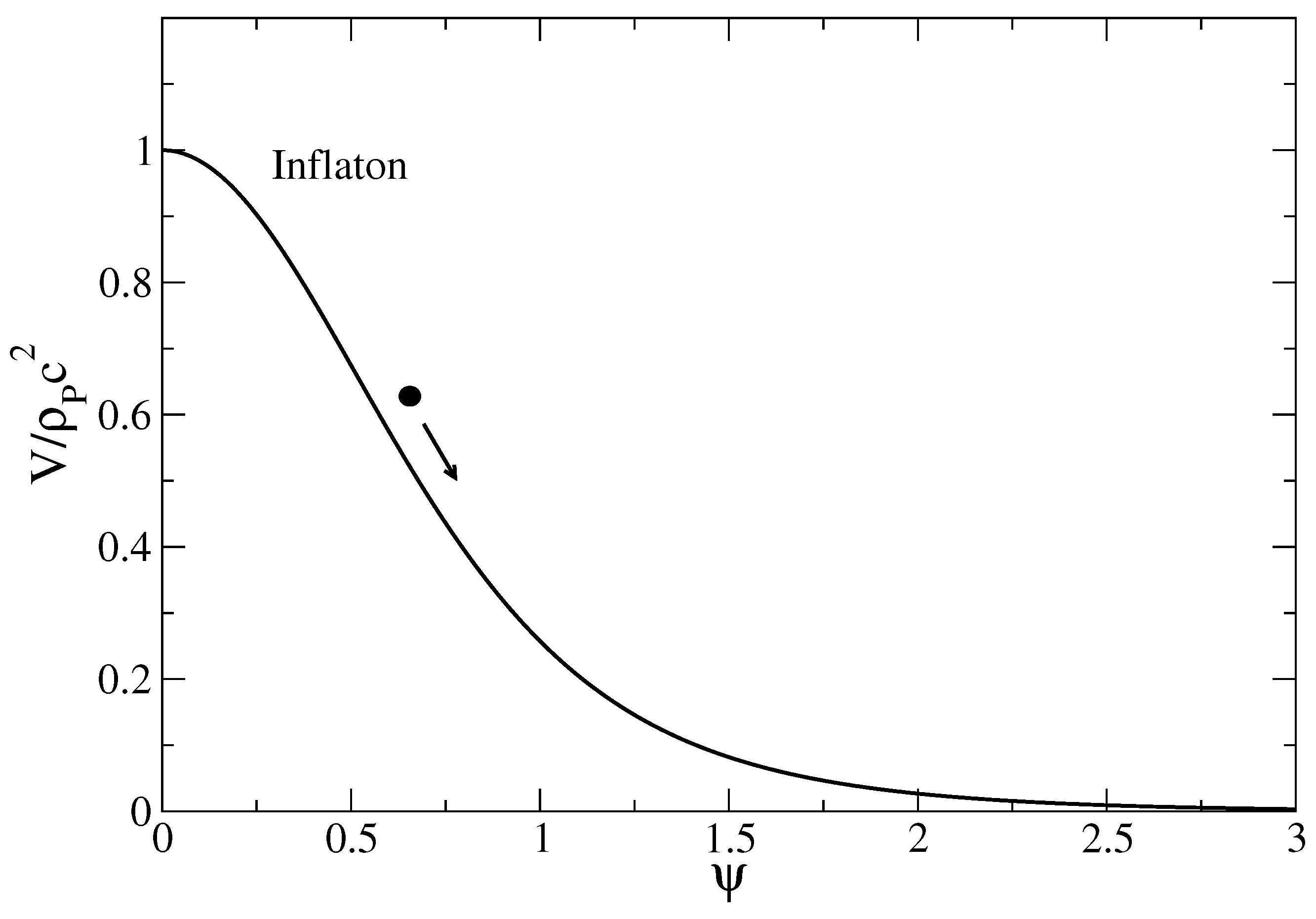
Figure 7.
Potential of the scalar field (inflaton) in the early universe. The field tends to run down the potential.
Figure 7.
Potential of the scalar field (inflaton) in the early universe. The field tends to run down the potential.
Figure 8.
Evolution of the scalar field (inflaton) as a function of time in the early universe. It displays a phase of early inflation before entering in the α-era.
Figure 8.
Evolution of the scalar field (inflaton) as a function of time in the early universe. It displays a phase of early inflation before entering in the α-era.
4. The Late Universe
In Reference [
30], we have proposed to describe the transition between the
α-era and the dark energy era in the late universe by a single equation of state of the form of Equation (
1) with
and
. It can be written as
Assuming
, the equation of continuity (
10) can be integrated into
where
and
is a constant of integration. We see that
corresponds to a lower bound (minimum value) for the density reached for
. Since this solution describes the late universe, it is natural to identify
with the cosmological density
. As a result, the equation of state (
45) can be rewritten as
For the sake of simplicity, and for definiteness, we shall select the index
. The general case
has been treated in [
30] and leads to qualitatively similar results. Therefore, we propose to describe the transition between the
α-era and the dark energy era in the late universe by a single equation of state of the form
where
is the cosmological density. This equation of state corresponds to a generalized polytropic equation of state (
1) with
and
. It can be viewed as the “symmetric” version of the equation of state (
18) in the early universe. For
, we recover the linear equation of state
. For
, we get
corresponding to the dark energy. The relation in Equation (
46) between the density and the scale factor becomes
The characteristic scale
marks the transition between the
α-era and the dark energy era. The equation of state (
48) interpolates smoothly between the
α-era (
and
) and the dark energy era (
and
). It provides therefore a “unified” description of the
α-era and dark energy era (de Sitter) in the late universe. This amounts to summing the density of these two phases. Indeed, Equation (
49) can be rewritten as
At
we have
so that
. Writing
, where
is the present value of the scale factor and
is the present density of the
α-fluid, and using the asymptotic expression
, we find that the transition scale factor
is determined by the relation
. On the other hand, comparing Equations (
19) and (
49) in the
α-era
(
i.e.,
) where the two equations of state overlap, we get
.
The equation of state parameter
and the deceleration parameter
q are given by
The velocity of sound
is given by
As the universe expands from
to
, the density decreases from
to
, the equation of state parameter
w decreases from
α to
, the deceleration parameter
q decreases from
to
, and the ratio
remains constant with the value
α (see Figures 1 and 5 of [
30]).
4.1. The Dark Energy Era: Late Inflation
When
, the density tends to a minimum value
and the pressure tends to
. The cosmological density
(dark energy) represents a fundamental lower bound for the density. A constant value of the density
gives rise to a phase of late inflation (accelerating expansion). It is convenient to define a cosmological time
and a cosmological length
. These are the counterparts of the Planck scales for the late universe (see Appendix B of [
30]). From the Friedmann equation (
12), we find that the Hubble parameter is constant
. Numerically,
. Therefore, the scale factor increases exponentially rapidly with time as
This exponential growth corresponds to the de Sitter solution [
1]. The timescale of the exponential growth is the cosmological time
. This solution exists at any time in the future (
and
for
), so there is no future singularity [Note 7: This is not the case of all cosmological models. In a “phantom universe” [
52,
53,
54,
55,
56,
57,
58,
59,
60,
61,
62,
63,
64,
65,
66,
67,
68,
69], violating the null dominant energy condition (
), the density increases as the universe expands. The models based on phantom dark energy usually predict a future singularity in which the scale factor, the energy density, and the pressure of the universe become infinite in a finite time. This would lead to the death of the universe in a singularity called Big Smash [
54], Big Rip, or Cosmic Doomsday [
53]. Contrary to the Big Crunch, the universe is destroyed not by excessive contraction but rather by excessive expansion. Every gravitationally bound system (e.g., the solar system, the Milky Way, the local group, galaxy clusters) is dissociated before the singularity [
53,
59], and the black holes gradually lose their mass and finally vanish at the Big Rip time [
60,
61,
62]. This scenario allows the explicit calculation of the rest of the lifetime of the universe. Actually, as we approach the singularity, the energy scale may grow up to the Planck scale, giving rise to a second quantum gravity era. Eventually, quantum effects may moderate or even prevent the singularity [
63]. It has also been proposed that, before reaching the Big Rip singularity, the universe could be swallowed by a wormhole [
72]. This is due to the accretion of the ever-increasing phantom energy by the wormhole. This accretion induces an increase of the wormhole throat so rapid that the size of the wormhole throat becomes infinite in a finite time preceding the Big Rip. As a result, the wormhole can engulf the entire universe before it reaches the Big Rip singularity. The wormhole would then act as a spacetime tunnel (Einstein-Rosen bridge) allowing the universe to pass to another, more gentle, universe without future singularity. This could be a way to escape the programmed death of the universe. This has been called the Big Trip. The possibility that we live in a phantom universe is not excluded by the observations. Indeed, observational data indicate that the equation of state parameter
w lies in a narrow strip around
, possibly being below this value. It is important to stress, however, that the phantom models with
do not necessarily lead to finite-time future singularities, as discussed in [
73]. For example, the scale factor and the density may increase indefinitely and become infinite in infinite time. This has been called Little Rip [
69]. In these models, the black holes disappear in infinite time while the wormhole’s throat still becomes infinite in a finite time. The phantom models without future singularity are attractive from the physical viewpoint because the occurrence of a finite time singularity may lead to some inconsistencies.].
4.2. The α-era
When
, we recover the equation
corresponding to the pure linear equation of state
. When
, the Friedmann equation (
12) yields
We then have
During the
α-era, the scale factor increases algebraically as
and the density decreases algebraically as
.
4.3. The General Solution
For the equation of state (
48), the density is related to the scale factor by Equation (
49). It is possible to solve the Friedmann equation (
12) with the density-radius relation of Equation (
49) analytically. Introducing
, we obtain
which can be integrated into [
30]:
The density is then given by
For
, Equation (
59) reduces to Equation (
56) and for
we obtain Equation (
54) with a prefactor
.
The time
corresponding to the transition between the
α-era and the dark energy era is obtained by substituting
in Equation (
59). On the other hand, according to Equation (
51), we find that the universe is decelerating when
(
i.e.,
) and accelerating when
(
i.e.,
) where
and
. The time
at which the universe starts accelerating is obtained by substituting
in Equation (
59). This corresponds to the time at which the curve
presents an inflexion point. For
(radiation), this inflexion point
coincides with
(
). For
the two points differ.
4.4. The Pressure
The pressure is given by Equation (
48). Using Equation (
49), we get
For
, the pressure decreases algebraically during the
α-era and tends to a negative constant value
for
. The point at which the pressure vanishes (
) corresponds to
and
. For
, the pressure is a constant
. At the transition point
, we have
. At the acceleration point
, we have
.
4.5. The Evolution of the Late Universe
When
, the universe is in the
α-era. Its radius increases algebraically as
while its density decreases algebraically as
. For
, the expansion of the universe is decelerating. When
, the universe is in the dark energy era. It undergoes a phase of accelerating expansion (late inflation) during which its radius increases exponentially rapidly with time while its density remains constant and equal to the cosmological density
. The Hubble constant, the Hubble time, the Hubble radius, and the density of the present universe are
,
,
, and
. For
(pressureless matter), the transition between the matter era and the dark energy era takes place at
,
, and
[
30]. The moment at which the universe starts accelerating corresponds to
,
, and
. The age of the universe is
(
if we use a more precise value of
[
30]). The present values of the deceleration parameter and of the equation of state parameter are
and
. The evolution of the scale factor and density as a function of time are represented in
Figure 9,
Figure 10,
Figure 11 and
Figure 12 in logarithmic and linear scales (the figures correspond to pressureless matter
).
Figure 9.
Evolution of the scale factor a with the time t in logarithmic scales. This figure clearly shows the transition between the α-era and the dark energy era (de Sitter). In the α-era, the radius increases as . In the dark energy era, the radius increases exponentially rapidly on a timescale of the order of the cosmological time . This corresponds to a phase of late inflation. The universe is decelerating for and accelerating for . The transition between the α-era and the dark energy era takes place at .
Figure 10.
Evolution of the scale factor a with the time t in linear scales.
Figure 10.
Evolution of the scale factor a with the time t in linear scales.
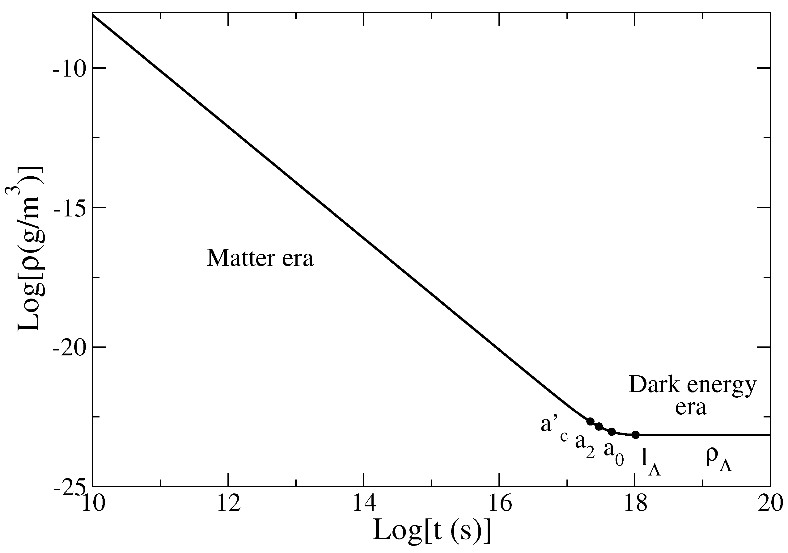
Figure 11.
Evolution of the density ρ with the time t in logarithmic scales. In the α-era, the density decreases as . During the late inflation (accelerating expansion), the density remains approximately constant with the cosmological value representing a lower bound.
Figure 11.
Evolution of the density ρ with the time t in logarithmic scales. In the α-era, the density decreases as . During the late inflation (accelerating expansion), the density remains approximately constant with the cosmological value representing a lower bound.
Figure 12.
Evolution of the density ρ with the time t in linear scales. General relativity (cosmological constant) limits the decay of the density to the cosmological value .
Figure 12.
Evolution of the density ρ with the time t in linear scales. General relativity (cosmological constant) limits the decay of the density to the cosmological value .
4.6. Scalar Field Theory
In alternative theories to the cosmological constant, the dark energy is usually described by a scalar field, defined by Equations (
33) and (
34), called quintessence [
12,
13,
14,
15,
16,
17,
18,
19,
20,
21,
22,
23,
24]. Using standard techniques [
7,
49], we find that the quintessence potential corresponding to the equation of state (
48) is (see Section 8.1 of [
30]):
where we have defined
For
,
For
,
For
, the scalar field potential
is constant. We can also show [
30] that the relation between the scalar field and the scale factor is
The end of the
α-era, and the beginning of the dark energy era, corresponds to
, hence to
. Combining Equations (
48), (
49) and (
66), we find that the energy density and the pressure of the universe are related to the scalar field by
Using Equation (
66), and the results of the previous sections, we can obtain the temporal evolution of the scalar field. For
, using Equation (
56), we get
For
, using Equation (
54) with the prefactor
, we get
More generally, using Equation (
59), the evolution of the scalar field
in the late universe is given by
These results are illustrated in
Figure 13 and
Figure 14 for
(pressureless matter).
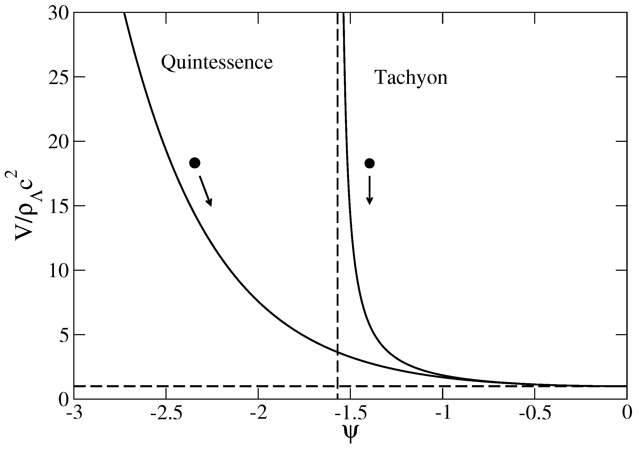
Some authors have proposed to represent the dark energy by a rolling tachyon condensate appearing in a class of string theories [
25]. A tachyonic scalar field [
26,
27,
28] has an equation of state
with
. This scalar field evolves according to the equation
The tachyonic field tends to run down the potential towards lower energies. The density and the pressure of the universe are related to the tachyonic field by
Figure 13.
Potential of the quintessence field and tachyonic field in the late universe. The field tends to run down the potential.
Figure 13.
Potential of the quintessence field and tachyonic field in the late universe. The field tends to run down the potential.
Figure 14.
Evolution of the quintessence field and tachyonic field as a function of time in the late universe.
Figure 14.
Evolution of the quintessence field and tachyonic field as a function of time in the late universe.
Let us consider the equation of state (
48) with the specific index
(pressureless matter). Since
is between
and 0, the equation of state (
48) can be associated with a tachyonic field. Using standard techniques [
7,
49], we find that its potential is (see Section 8.2 [
30]):
where we have defined
For
,
For
,
We can also show [
30] that the relation between the scalar field and the scale factor is
The end of the matter-era (
), and the beginning of the dark energy era, corresponds to
, hence to
. Combining Equations (
48), (
49) and (
77), we find that the energy density and the pressure of the universe are related to the scalar field by
Using Equation (
77), and the results of the previous sections, we can obtain the temporal evolution of the scalar field. In the matter era (
), using Equation (
56), we get
In the dark energy era (
), using Equation (
54) with a prefactor
, we get
More generally, using Equation (
59), the evolution of the tachyonic field
in the late universe is given by
These results are illustrated in
Figure 13 and
Figure 14 for
(pressureless matter).
Remark: The canonical scalar field potential of Equation (
62) describing the transition between the
α-era and the dark energy era involves hyperbolic functions. It corresponds to the scalar field potential associated with the generalized Chaplygin gas (see Note 1) [
37,
38,
39,
40,
41,
42,
43,
44,
45]. Other types of hyperbolic scalar field potentials have been introduced in the past. The first potential with hyperbolic functions driving the observed acceleration of the universe was proposed by Sahni and Wang [
74] and has been confronted to the observations in [
75]. Related potentials were considered in [
76,
77,
78]. Models with hyperbolic potentials exploiting dynamical Noether symmetries of the field equations and admiting analytical solutions were constructed and compared with cosmological data in [
79], finding a good agreement. On the other hand, the tachyonic scalar field potential of Equation (
73) describing the transition between the
α-era and the dark energy era involves trigonometric functions. A tachyonic field with a trigonometric potential was proposed in [
80] to describe the transition between dark matter and dark energy. Interestingly, this model admits different solutions depending on the initial condition. It can either describe an eternally expanding universe or lead to a future finite time singularity, called Big Brake, which is characterized by an infinite deceleration. This model has been recently subjected to several cosmological tests in [
81].
6. Conclusions
We have constructed a cosmological model based on the quadratic equation of state (
2). This equation of state describes the evolution of a universe presenting a phase of early inflation (Planck era), a phase of decelerating expansion (
α-era), and a phase of late accelerating expansion (de Sitter era). An interest of this model is its simplicity (while being already quite rich) and the fact that it admits a fully analytical solution (see Equation (
106)). It provides a particular solution of the Friedmann equations. In addition, it is in qualitative agreement with the evolution of our own universe. Finally, it admits a scalar field interpretation based on an inflaton, quintessence, or tachyonic field.
This model does not present any singularity and exists “eternally” in the past and in the future, so that it has no origin nor end (we call it aioniotic universe). In particular, the phase of early inflation avoids the Big Bang singularity and replaces it by a sort of second order phase transition where the non-zero value of the Planck constant ℏ plays the same role as finite size effects in statistical mechanics. Of course, it is probably incorrect to extrapolate the results in the infinite past since our model is purely classical, or semi-classical, and does not take quantum gravity into account. In our model, the universe starts from but, for , its size is less than the Planck length . In the Planck era, the classical Einstein equations may be incorrect and should be replaced by a theory of quantum gravity that still has to be constructed.
Another interest of this model is that it describes the early universe and the late universe in a symmetric manner. The early universe is described by a polytrope
and the late universe by a polytrope
. The mathematical formulae are then strikingly symmetric (we sum the inverse of the densities in the early universe and we sum the densities in the late universe). Furthermore, the Planck density
in the early universe plays the same role as the cosmological density
in the late universe. They represent fundamental upper and lower density bounds differing by 122 orders of magnitude. They lead to phases of early and late inflation with very different timescales
and
. The densities
and
(together with
α) appear as the coefficients of the equation of state (
2). Therefore, this equation of state provides a “unification” of vacuum energy and dark energy.
A limitation of this equation of state is that it cannot describe the transition between the radiation era and the matter era because they are both described by a linear equation of state
with
and
respectively. Therefore, the equation of state (
2) with
describes a universe without matter while the equation of state (
2) with
describes a universe without radiation. A better model can be achieved by letting
vary with time and decrease smoothly from
to 0. Alternatively, we can “unify” vacuum energy + radiation + dark energy into a “generalized radiation” described by the equation of state (
2) with
and treat baryonic matter and dark matter as independent species described by the equations of state
and
. This general approach (see
Section 5.8) allows us to describe the complete evolution of the universe (inflation + radiation + matter + acceleration). It leads to an interesting generalization of the ΛCDM model where Equation (
107) is replaced by Equation (
110). As a result, our model generalizes the standard ΛCDM model by incorporating naturally a phase of early inflation that avoids the primordial singularity. Furthermore, it describes the early inflation and the late acceleration simultaneously with a single equation of state that unifies vacuum energy and dark energy, and a single scalar field potential that unifies the inflaton potential and the quintessence potential (see
Appendix A).
Dark matter is usually described by a pressureless equation of state
. This leads to the famous Einstein-de Sitter (EdS) model. However, there are indications that dark matter may be described by an isothermal equation of state
with
[
48]. Therefore, it is useful to provide general results valid for arbitrary values of
α as we have done here. This allows us to describe either radiation (
), pressureless matter (
), or isothermal matter (
).
In this paper, for definiteness, we have selected the indices
and
in Equation (
82) to describe the early and the late universe respectively. As we have seen, the equation of state (
82) with
leads to results that coincide with the ΛCDM model in the late universe. This equivalence is not trivial since our approach is fundamentally different from the ΛCDM model (in particular this coincidence is not true anymore for
). Since the ΛCDM model provides a good description of the universe after the Planck era, this implies that observations tend to favor the value
of the polytropic index. This is a reason why we have selected this index. However, we can obtain more general models by taking
different from
. In particular, a value of
close to
may be consistent with the observations and may improve upon the ΛCDM model. In this respect, Asadzadeli
et al. [
95] have shown that the observations constrain the index
to be in the range
or
at
and
confidence levels, respectively. On the other hand, we have selected the index
in Equation (
82) to describe the inflation in the early universe. More general models of inflation can be obtained by selecting other values of
. The value of
could be determined from the measurements of the cosmic microwave background (CMB) radiation. Therefore, possible extensions of our study would be to consider the generalized equation of state (
82) with arbitrary values of
and
. General results valid for the asymptotic expressions (Equations (
17) and (
47)) of the equation of state (
82) in the early and late universe are given in [
29,
30,
31].
A weakness of our work is that we have not given a justification of the quadratic equation of state (
2) [Note 14: It would be of considerable interest to justify this equation of state from a microscopic model of radiation since we argued that this equation of state provides an effective model of “generalized radiation”. The quadratic equation of state (
18) and the analytical solution of Equation (
29) describing the phase of inflation were first given in [
96] in relation to Bose-Einstein condensates (BECs) with an attractive self-interaction (negative scattering length
). Although this BEC model may be too simplistic (see the discussion in Appendix B of [
29]), it shows how a quadratic equation of state with a negative pressure may arise in practice. We may also draw an analogy between the BEC model and the primeval atom of Lemaître [
97].]. However, since this equation of state is connected to the Chaplygin gas model, there is some hope that this equation of state could arise from fundamental theories since the original Chaplygin gas model [
37,
38,
39,
40,
41,
42,
43,
44,
45] is motivated by some works on string theory. It can be obtained from the Nambu-Goto (or Born-Infeld) action for
d-branes moving in a
-dimensional spacetime in the light-cone parametrization [Note 15: We also note that a theoretical justification of a polytropic equation of state of the form
with
for a perfect relativistic fluid in cosmology has been given recently by Kazinski [
98] in relation to the quantum gravitational anomaly.]. We may also argue that the quadratic equation of state (
2) (and its generalization in Equation (
82)) is the “simplest” equation of state that we can imagine in order to obtain a non singular model of universe (see the discussion in Section 7.4 of [
30]). This “simplest” model is in agreement with the known properties of our universe. It is interesting that these properties can be reproduced by an equation of state of the form
where the three coefficients are related to ℏ,
α, and Λ.
In this paper, the quadratic equation of state (
2) has been introduced heuristically in order to obtain a cosmological model that describes simultaneously a phase of inflation, a phase of decelerating expansion, and a phase of acceleration. The Planck constant ℏ and the cosmological constant Λ are interpreted as two fundamental constants fixed by nature that appear in the coefficients of this equation of state. In a sense, this equation of state can be viewed as a simple interpolation formula between different, well-motivated, equations of state. Interpolation formulae are often useful in physics and the equation of state (
2) is also interesting in this respect.
The next step would be to study the growth of perturbations in our model. In particular, it would be important to confront the model of inflation based on the polytropic equation of state (
15) to the Planck 2015 data set. In this respect, it may be necessary to use the scalar field interpretation instead of the hydrodynamic interpretation because it is known that, although the hydrodynamic and scalar field equations coincide at the background level, they may show differences at the level of the perturbations. A first study has been made in this direction by Freitas and Gonçalves [
94] using our model of inflation. They studied the primordial quantum fluctuations in the slow-roll approximation and calculated the scalar perturbations, the scalar power spectrum, and the spectral index. They obtained encouraging results, but some of their results need to be further developed. This will be considered in future works.
Remark: In this paper, we have proposed to describe the complete evolution of the universe (early and late inflation) by the quadratic equation of state (
2). A quadratic equation of state aiming at describing the late acceleration of the universe has been considered in [
63,
64,
99,
100] and compared to the observations by Sharov [
101]. Sharov mentions that a quadratic equation of state with a positive coefficient in front of
can lead to past singularities. In the present paper, we have considered a quadratic equation of state with a small negative coefficient in front of
(of the order of
), so that the quadratic term accounts for the early inflation, not for the late acceleration. This is why we do not have past singularities in our model (the universe exits at any time in the past). The possibility of past singularities when the coefficient in front of
is positive is discussed in [
29].


