Two Novel Approaches to the Hadron-Quark Mixed Phase in Compact Stars
by
 , , , and
Vahagn Abgaryan
1 ,
,
David Alvarez-Castillo
2,*,
Alexander Ayriyan
1,*,
David Blaschke
2,3,4 and
Hovik Grigorian
1,5 1
Laboratory for Information Technologies, Joint Institute for Nuclear Research, Joliot-Curie Street 6, Dubna 141980, Russia
2
Bogoliubov Laboratory for Theoretical Physics, Joint Institute for Nuclear Research, Joliot-Curie Street 6, Dubna 141980, Russia
3
Institute of Theoretical Physics, University of Wroclaw, Max Born Place 9, 50-204 Wroclaw, Poland
4
National Research Nuclear University (MEPhI), Kashirskoe Shosse 31, Moscow 115409, Russia
5
Department of Physics, Yerevan State University, Alek Manukyan Str. 1, Yerevan 0025, Armenia
*
Authors to whom correspondence should be addressed.
Universe 2018, 4(9), 94; https://0-doi-org.brum.beds.ac.uk/10.3390/universe4090094
Submission received: 23 July 2018
/
Revised: 31 August 2018
/
Accepted: 31 August 2018
/
Published: 5 September 2018
(This article belongs to the Special Issue Compact Stars in the QCD Phase Diagram)
Abstract
:First-order phase transitions, such as the liquid-gas transition, proceed via formation of structures, such as bubbles and droplets. In strongly interacting compact star matter, at the crust-core transition but also the hadron-quark transition in the core, these structures form different shapes dubbed “pasta phases”. We describe two methods to obtain one-parameter families of hybrid equations of state (EoS) substituting the Maxwell construction that mimic the thermodynamic behaviour of pasta phase in between a low-density hadron and a high-density quark matter phase without explicitly computing geometrical structures. Both methods reproduce the Maxwell construction as a limiting case. The first method replaces the behaviour of pressure against chemical potential in a finite region around the critical pressure of the Maxwell construction by a polynomial interpolation. The second method uses extrapolations of the hadronic and quark matter EoS beyond the Maxwell point to define a mixing of both with weight functions bounded by finite limits around the Maxwell point. We apply both methods to the case of a hybrid EoS with a strong first order transition that entails the formation of a third family of compact stars and the corresponding mass twin phenomenon. For both models, we investigate the robustness of this phenomenon against variation of the single parameter: the pressure increment at the critical chemical potential that quantifies the deviation from the Maxwell construction. We also show sets of results for compact star observables other than mass and radius, namely the moment of inertia and the baryon mass.
1. Introduction
The understanding of the properties of dense matter in compact star interiors is a subject of current research. Recently, great progress in this direction has been achieved by the detection of the gravitational radiation that emerged from the inspiral phase of two coalescing compact stars, an event named GW170817 [1]. Since it was observed in all other bands of the electromagnetic spectrum, it marked the birth of multi-messenger astronomy. Among the various obtained results, GW170817 has shed light on the properties of the equation of state (EoS) of compact star matter, namely on its stiffness, since through the constraints on the tidal deformability parameter [2] from the LIGO-Virgo Collaboration (LVC) results one could estimate the maximum radius of a 1.4 M⊙ compact star to km [3] and maximum mass of nonrotating compacts stars M⊙ [4]. Of great scientific interest is the phenomenon of a phase transition from hadronic matter to a deconfined quark phase in hybrid compact stars. Those stars are comprised of a deconfined quark matter core surrounded by a hadronic mantle. The nature of the deconfinement transition is a matter of debate [5,6]. Whether it exhibits a jump in the thermodynamic variables or represents a crossover (1 is a question that is addressed to both, laboratory experiments as well as compact star observations. The possibility of a mixed phase in neutron stars arises. Standard approaches to describe such a domain of coexistence of competing phases are: (i) the Maxwell construction (for just one chemical potential) which leads to sharp phase boundaries due to constant pressure throughout the mixed phase; (ii) the Gibbs construction (for several chemical potentials corresponding to different conserved quantities) [7], where the pressure changes in the mixed phase which is quasi homogeneous due to the neglect of surface tension effects; and (iii) the constructions with finite size structures of different shapes (“pasta phases” [8]) due to surface tension and Coulomb effects that are mainly modeled with the approximation of sharp surfaces and the surface tension as a free parameter. The adequate description of the letter is a complicated problem where the geometrical properties of the structures, as well as transitions between them, must be taken into account (different methodologies can be found in [9,10,11,12,13,14,15]). In the case of the hadron-quark interface, the procedure is well explained in [16] (see also [15] for a recent work); one models several geometrical structures and finds the energetically most favorable ones in different density regions inside compact stars. The occurrence of structures introduces surfaces separating the phases coexisting in the mixed phase. The value of the surface tension determines the size of the structures and thus the amount of surface per volume that can optimally be afforded. While for a vanishing surface tension the mixed phase becomes quasi homogeneous and is largest, a high value of surface tension results in a single surface as for the Maxwell construction that corresponds to , see Figure 1. The quantitative relation between and the surface tension is under investigation [17].
In this work we take a different route and introduce two types of phenomenological interpolations which aim at mimicking the thermodynamic behaviour of those geometrical structures while simultaneously exploring the whole corresponding density range in a unified way. A first realization of the idea to describe the transition from the hadronic to the quark matter phase of matter in neutron stars by an interpolation in order to model a crossover-like behaviour was carried out in [18] and followed up in Refs. [19,20], where the jump of the EoS was replaced by a smooth behaviour using as an ansatz a tangens hyperbolicus function.
The mixed phase constructions in this work are developed exclusively for stellar matter where the conditions of charge neutrality and beta equilibrium apply. These constraints allow to express the other chemical potentials in terms of the baryon one. Therefore, only the baryon chemical potential remains as the single independent thermodynamic variable. The pressure as a function of as shown in Figure 1 can be viewed as a projection from a higher dimensional space spanned by the pressure and several other chemical potentials onto the plane where the resulting function is subject to modeling within our simplified approach to mimic the effect of pasta structures in the mixed phase.
A systematic and thermodynamically consistent formulation was recently given in [21,22], where a parabolic interpolation function was introduced to replace the behaviour of the hybrid EoS for a Maxwell transition. We shall denote this procedure as the replacement interpolation method (RIM). The resulting hybrid EoS was then used to study the effect of the mixed phase on the properties of compact stars. A second realization of this concept has been worked out recently in [23], where instead of replacing the hadronic and quark matter branches of the hybrid EoS in the limits (see Figure 1) a mixing of these branches is defined using switch functions and a bell-shaped function for the pressure increment with an amplitude , where is the critical pressure of the Maxwell construction. This procedure is denoted as the mixing interpolation method (MIM) in [23]. The free parameter occurs in both methods with an equivalent influence on the behaviour of the EoS in the mixed phase region, in particular on its extension, see Figure 1. We would like to note that in both methods a negative value of would signal that a Maxwell construction using both input EoS for hadronic matter and for quark matter would not make sense because it would describe a transition from quark matter at low densities (where is not trustworthy) to hadronic matter at high densities (where is not trustworthy). For a discussion of this situation, see Ref. [24].
In this work we present a comparative study of the RIM and MIM approaches to construct mixed phases of the quark-hadron phase transition that mimic the thermodynamic behaviour of pasta phases. We discuss the similarities and differences of these two approaches and apply them to obtain a hybrid EoS under neutron star constraints for which we discuss the resulting hybrid star sequences and their properties. While the first approach (RIM) is rather intuitive and simple to realise as its properties just depend on the order of interpolating polynomial, the second approach (MIM) is based on a procedure of “mixing” the EoS of the two phases in the coexistence region and reminds in its properties on the physics of substitutional compounds as in the crust of compact stars, resulting in an intermediate stiffening effect.
The paper is structured as follows. In Section 2 we start with the reference EOS for the present study, for which a four-polytrope ansatz is employed which features a hadronic phase (first polytrope), a constant pressure polytrope resembling a strong first order phase transition as described by a Maxwell construction (second polytrope) and two polytropes for quark matter phases at high densities. Next, in Section 3, we introduce the RIM and MIM approaches to construct mixed phases when two reference EoS for the low-density (hadronic) and high-density (quark matter) phases are given. We discuss the speed of sound as the key characterizing property of the family of obtained hybrid EoS. Subsequently, in Section 4, we discuss the similarities and differences between the hybrid star EoS of both approaches and show results for the macroscopic properties of compact stars. We motivate these results by the feasibility of detection by multi-messenger astronomy. Consequently, future detections of gravitational wave radiation emitted by of NS–NS or NS–BH mergers shall provide new constraints on both the star mass and radius. Moreover, the determination of the fate of the merger, whether it evolves via a prompt or delayed collapse into a black hole, can be used as an independent estimate on the mass and radius, as proposed in [25]. Up to now, tests for the current compact star models with the at present still single compact star merger event have been performed, e.g., in [22,23,26].
2. Hybrid Star EoS with a Third Family and High-Mass Twins
Compact stars are traditionally divided into white dwarf (first family) and neutron star (second family) branches. Hybrid stars whose equation of state undergoes a sufficiently strong first order phase transition (large jump in energy density ) can populate a third family branch in the mass-radius diagram, separated from the second one by a sequence of unstable configurations. As a consequence, there appear so called mass twin configurations: the second and third family solutions overlap within a certain range of masses while the radii of any two stars with the same mass (mass twins) are very different. If the mass-twin phenomenon occurs at high masses ∼2 M⊙ then one speaks of high-mass twin (HMT) stars [27]. Depending on the critical pressure of the phase transition, the mass-twin phenomenon can occur also at lower masses such as the typical binary radio pulsar mass of ∼1.35 M⊙, see [22,23,26], so that the corresponding twin star configuration become of relevance for the interpretation of GW170817. In the latter case, a mass ratio of the merger would not entail that the merging stars have the same radii and internal structure! Would the mass-twin phenomenon (at whatever mass) be observed, this would entail that the QCD phase diagram has to possess at least one critical endpoint since for the study of the cold region of the QCD phase diagram the existence of a first order phase transition between hadron to quark matter had to be concluded. Since the high temperature region of the QCD diagram is known to feature a crossover transition, compact stars can serve as a probe of the existence of a critical end point [28] and provide insight into the properties of matter in heavy ion collision conditions [29].
In order to study the effects of pasta phases at the hadron-quark matter interface in hybrid star interiors, we consider a piecewise polytropic EoS as previously used in various works [3,30,31,32,33]. The polytropic representation used in the present work consists of four segments of matter at densities higher than saturation density fm−3 ().
Each density region is labelled by with prefactor and polytropic index . HMT stars require a rather stiff nucleonic EoS which here is represented by the first polytrope. The hadron-quark matter first-order phase transition is described by the second polytrope with constant pressure and vanishing polytropic index (). At higher densities the polytropes 3 and 4 represent a rather stiff quark matter EoS. The parameters for this HMT realisation are given in Table 1.
For the present applications to thermodynamically consistent interpolating constructions we need to convert the EoS (1) to the form [33]
valid for the respective regions (phases) , where for the constant pressure region this formula collapses to because of . The masses represent the effective masses of the constituent degrees of freedom in the phase i. For example, in the hadronic region, , where is the nucleon mass. At higher densities, this corresponds to effective quark masses. For applying the MIM below, it will be important that the pressure of the hadronic phase () valid for can be extrapolated to the neighbouring quark matter phase () where and vice-versa.
HMT star EoS fulfil the Seidov conditions over quantity values at the phase transition [34]
for the third family of compact stars to exist. These conditions determine the existence of a gap on the mass-radius relation, therefore separating the third family of compact stars from the second one. Once a small region of different matter appears in the centre of the star, the effect can be studied by perturbation theory [34] or by linear response theory [35,36]. The result is that if the Seidov conditions are satisfied, any increase in the central pressure will lead to an instability against oscillations precisely of the same type that happens when the maximum mass is exceeded in the mass-radius relation. The choice of parameters for this EoS corresponds to a sufficiently stiff high-density region in order to prevent gravitational collapse while at the same time not violating the causality condition for the speed of sound . See [33] for details.
3. Mixed Phase Constructions
In this section we present the details of the interpolation descriptions for the mixed phase between the hadronic and quark matter phases. For this purpose we consider the chemical potential dependent pressures of both the hadronic () and the neighbouring quark matter () phases: , , respectively. As mentioned above, our polytropic HMTs EoS features a first order phase transition implemented in the form of a Maxwell construction at a critical chemical potential value where pressures for both phases are equal:
thus both phases are in thermodynamic equilibrium.
3.1. The Replacement Interpolation Method (RIM)
In this mixed phase approach the relevant regions of both, the hadronic and quark matter EoS around the Maxwell critical point () are replaced by a polynomial function defined as
where is a free parameter representing additional pressure of the mixed phase at . Generally, the ansatz (5) for the mixed phase pressure is an even order (, k = 1,2, …) polynomial and it smoothly matches the EoS at and up to the k-th derivative of the pressure,
where parameter values (, and , for ) can be found by solving the above system of equations, leaving one parameter () as a free parameter of this method.
As usual, the parameters , , and are found from the following system of equations involving quantities at the borders of the mixed phase,
It is evident that the order of the interpolating function (5) will determine whether or not there are discontinuities for the derivatives of the function .
For instance, the square of the speed of sound,
involves the second derivative of the pressure with respect to since , see Figure 2. The result is that for the function (5) exhibits a clear discontinuity in the speed of sound at and , whereas in between these borders, the speed of sound slightly increases relative to the case of the Maxwell construction for which in the mixed phase region. For , the mixed phase pressure (5) allows for a continuous speed of sound. However, it is connected at and to the speed of sound outside these borders with a jump in its derivative. At the order and higher the speed of sound behaves smoothly without a jump in its derivative. However, the sharp change in the speed of sound remains as a feature of matter around the transition points and distinctive of a first order phase transition. Moreover, the effect of taking into account the contribution of the higher order polynomials is a softening at the transition that can be associated with crossover–type phase transitions.
3.2. The Mixing Interpolation Method (MIM)
This approach has recently been defined in Ref. [23], where the interpolation ansatz was based on trigonometric functions. Here we will use instead a polynomial ansatz for the interpolation that consists of a pair of functions and that will switch off and on the hadronic and quark parts of the equation of state, as well as an additional compensating function in order to eliminate thermodynamic instabilities, see Figure 3. This interpolation is applied in the p − plane within the range .
The pressure that interpolates between the hadron and quark phase at the phase transition reads
Even though and might be any switching functions, our choice of definition consists of the following pair of left and right side polynomials:
that together with the complementary functions and will complete the switch functions. The above coefficients , , and can be determined by the following conditions
where the value of is chosen for symmetric convenience. Consequently, the switching functions are defined as
and furthermore obey .
In order to construct a proper dimensionless function we introduce
consisting of the functions
whose coefficients are determined by the conditions
Regarding as the only free external parameter, up to this moment we have 10 unknowns and eight independent equations which leave us with the possibility to fix the second order derivative of P at and in the following way:
4. Results
4.1. Hybrid Star EoS with Mixed Phases
The two interpolation methods presented above result in a thermodynamically consistent EoS. Knowing that , the thermodynamic identity used to derived all the needed variables at zero temperature reads
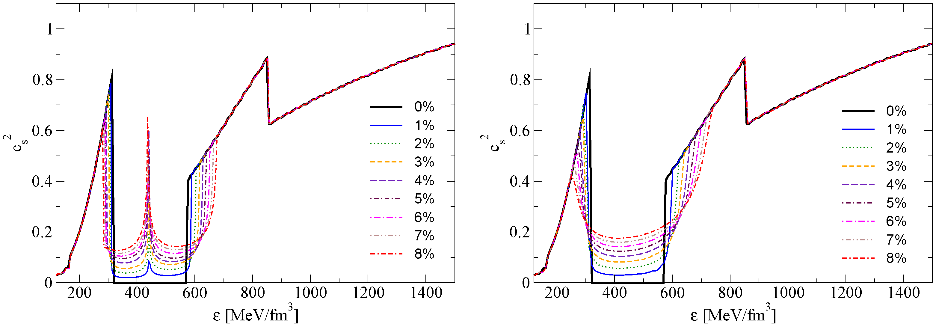
Figure 4 shows the resulting mixed phase interpolations for both approaches characterised by the dimensionless pressure increment that ranges from 1 to , where reproduces the Maxwell construction. Figure 5 shows pressure values depending on energy density. The first order phase transition via a Maxwell construction corresponds to the case with the pressure being constant in the mixed phase region. Furthermore, Figure 6 shows the squared speed of sound for both approaches where the difference between them becomes obvious: while the MIM shows a peak in the mixed phase region the RIM shows a rather structureless behaviour in this region. This feature is a direct consequence of the functional form of the interpolation implemented by the two methods.
4.2. Compact Star Sequences
In order to compute the compact star internal pressure (energy density) profiles leading to mass-radius relations, we solve the Tolman–Oppenheimer–Volkoff (TOV) equations [37,38] derived in the framework of General Relativity for a static, spherically-symmetric compact star
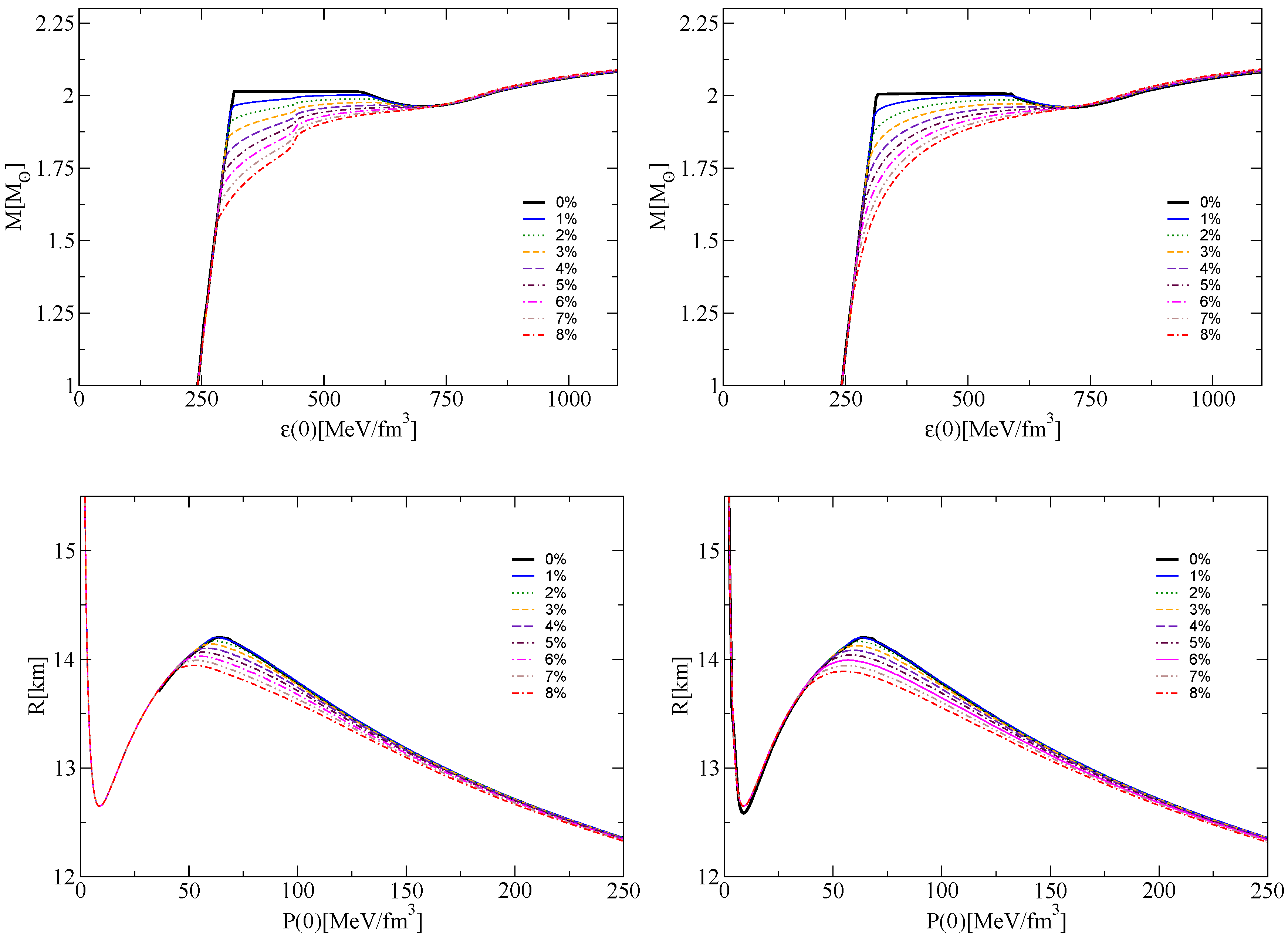
with the boundary conditions , M(0) = 0 and that serve to determine the total stellar mass M and total stellar radius R once a central pressure (and with it the central energy density because is known) is given as input. By increasing the central energy density values, a whole sequence of star configurations up to the one with the maximal mass can be obtained, thus populating the mass-radius diagram. Figure 7 shows compact star sequences for all models characterised by the value for both, the MIM and RIM approaches together with up-to-date constraints from astrophysical measurements. We can notice that for the lower values of the HMT phenomenon persists regardless which mixed phase interpolation method has been applied. In Figure 8 we show the mass versus central energy density and the radius versus central pressure for both interpolation methods. For the MIM one observes a trace of the intermediate stiffening effect in the mass versus central energy density which is absent for the RIM.
In addition, two other quantities of astrophysical interest are the total baryonic mass of the star that results from integrating the following equation
and similarly, its moment of intertia [42]
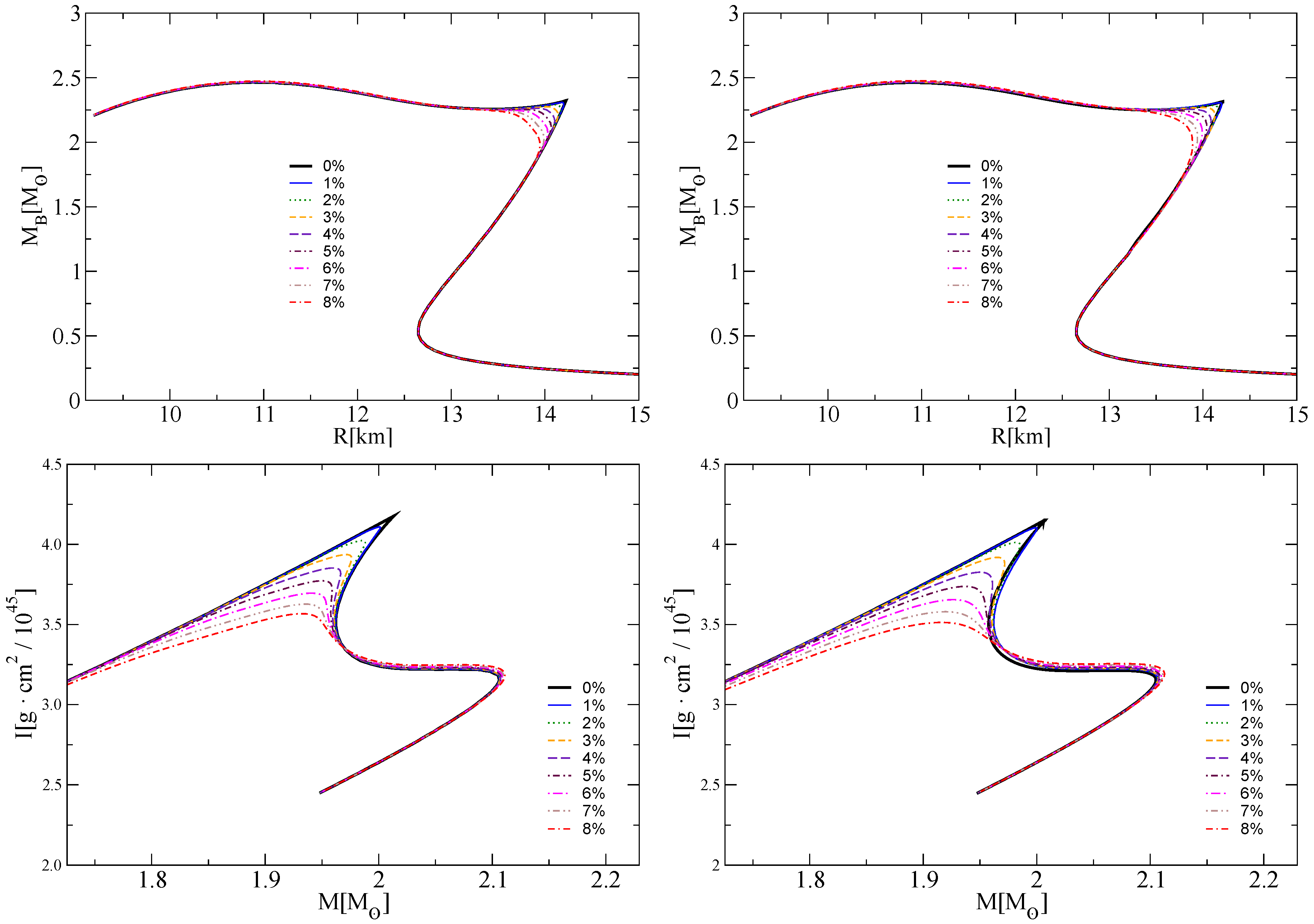
which are related to observational phenomena as well, like energetic emissions that might conserve baryon mass or moment of inertia dependent pulsar glitches. For a detailed discussion of the moment of inertia in the slow-rotation approximation, and for the hybrid star case see, e.g., [43,44,45], and references therein. In Figure 9 we show the baryon mass versus radius and and the moment of inertia versus gravitational mass for the compact star sequences obtained in this work with both interpolation methods. When increasing the pressure increment from to , the sharp edges which are obtained for the Maxwell construction case get washed out. One observes no qualitative difference between the MIM and the RIM in the patterns of these families of sequences. For , the second and third family branches in the versus R diagrams get joined so that neutron star and hybrid star configurations form a connected sequence and the HMT phenomenon get lost. This effect is reflected in the I vs. M diagrams by the loss of multiple values (the lowest branch up to the maximum mass of M⊙ shall be ignored because it is unstable). From the versus R diagrams one can read off which configuration on the hybrid star branch would be reached when the maximum mass neutron star configuration would collapse under conservation of baryon number. Comparing the gravitational masses of these two star configurations one can estimate the release of binding energy in this process, see Ref. [45].
5. Conclusions
In this work we have introduced two interpolation approaches to a mixed phase at the hadron-quark phase transition. An advantage of these two interpolation methods presented here over the construction employing hyperbolic tangent functions [19,20] is the finite extension in chemical potentials of the mixed phase between the hadronic and the quark EoS, whereas the latter strictly converges only at infinity.
While each approach uses a different functional form, both fulfil the same conditions at the border of the mixed phase. We have found that both methods can be distinguished by the behaviour of the speed of sound that they predict. The MIM approach motivated by the analogy with sequential phase transitions occurring for substitutional compounds in the neutron star crust finds an intermediate stiffening of the mixed phase EoS. The RIM approach does not exhibit this feature. In the case of the RIM approach, we have studied both a fourth and sixth order polynomial interpolation. We found that the latter connects the hadron and quark EoS smoothly up to second derivatives, which is visible in the smooth behaviour of the speed of sound. However, the differences in the neutron star properties for both polynomial orders are safely negligible.
The macroscopic properties of compact stars show, for both mixed phase constructions, a very similar systematic behaviour as the pressure increment is increased: the mass-radius relation smooths out, eliminating the gap between second and third branches, however, we have only considered the highest values. Up to the HMT phenomenon is robust against the mixed phase construction, regardless whether the MIM or RIM approach is used. For the mass versus central energy density, one observes a trace of the intermediate stiffening effect for the MIM which is absent for the RIM. For the other compact star quantities evaluated here, the baryonic mass and the moment of inertia, both interpolation methods display a similar type of behaviour when the pressure increment is varied.
The methods presented here can potentially be applied to the compact star crust-core transition as well. Just like at the hadron-quark boundary, the transition at the bottom of the crust may proceed via pasta phases dominated by Coulomb forces and surface tension effects [8]. Further astrophysical aspects of mixed phases inside neutron stars include potentially observable effects such as the rotational evolution, pulsar glitches, gravitational wave emission and cooling. They could be sufficiently sensible to the nature of the phase transition, proceeding via pasta phases or not, and thus provide potential signatures of the presence and extension of a mixed phase in compact stars.
Author Contributions
All authors have discussed the results presented in the article and contributed to its final form. The RIM was originally developed by A.A. and H.G. while D.A.-C. and D.B. developed the MIM. A.A. and V.A. generalized RIM for the higher order. V.A. made its realization and called to life H.G’s idea of polynomial switching functions. D.A.-C. calculated the compact star configurations.
Funding
This research was funded by the Russian Science Foundation grant number 17-12-01427. D.A.-C. is grateful NCN grant no. UMO-2014/13/B/ST9/02621 and the Bogoliubov-Infeld Program for collaboration between JINR Dubna and Polish Institutes.
Acknowledgments
The authors thank N. Yasutake, K. Maslov and D.N. Voskresensky for fruitful discussions on the features of hadron-quark mixed phase.
Conflicts of Interest
The authors declare no conflict of interest.
References
- Abbott, B.P.; Abbott, R.; Abbott, T.D.; Acernese, F.; Ackley, K.; Adams, C.; Adams, T.; Addesso, P.; Adhikari, R.X.; Adya, V.B.; et al. GW170817: Observation of gravitational waves from a binary neutron star inspiral. Phys. Rev. Lett. 2017, 119, 161101. [Google Scholar] [CrossRef] [PubMed]
- Hinderer, T.; Lackey, B.D.; Lang, R.N.; Read, J.S. Tidal deformability of neutron stars with realistic equations of state and their gravitational wave signatures in binary inspiral. Phys. Rev. D 2010, 81, 123016. [Google Scholar] [CrossRef]
- Annala, E.; Gorda, T.; Kurkela, A.; Vuorinen, A. Gravitational-wave constraints on the neutron-star-matter Equation of State. Phys. Rev. Lett. 2018, 120, 172703. [Google Scholar] [CrossRef] [PubMed]
- Rezzolla, L.; Most, E.R.; Weih, L.R. Using gravitational-wave observations and quasi-universal relations to constrain the maximum mass of neutron stars. Astrophys. J. 2018, L25, 852. [Google Scholar] [CrossRef]
- Alford, M.G.; Han, S.; Prakash, M. Generic conditions for stable hybrid stars. Phys. Rev. D 2013, 88, 083013. [Google Scholar] [CrossRef]
- Kojo, T. Phenomenological neutron star equations of state: 3-window modeling of QCD matter. Eur. Phys. J. A 2016, 52, 51. [Google Scholar] [CrossRef]
- Glendenning, N.K. First order phase transitions with more than one conserved charge: Consequences for neutron stars. Phys. Rev. D 1992, 46, 1274–1287. [Google Scholar] [CrossRef]
- Ravenhall, D.G.; Pethick, C.J.; Wilson, J.R. Structure of Matter below Nuclear Saturation Density. Phys. Rev. Lett. 1983, 50, 2066. [Google Scholar] [CrossRef]
- Voskresensky, D.N.; Yasuhira, M.; Tatsumi, T. Charge screening at first order phase transitions and hadron quark mixed phase. Nucl. Phys. A 2003, 723, 291–339. [Google Scholar] [CrossRef]
- Maruyama, T.; Chiba, S.; Schulze, H.J.; Tatsumi, T. Quark deconfinement transition in hyperonic matter. Phys. Lett. B 2008, 659, 192–196. [Google Scholar] [CrossRef] [Green Version]
- Watanabe, G.; Sato, K.; Yasuoka, K.; Ebisuzaki, T. Structure of cold nuclear matter at subnuclear densities by quantum molecular dynamics. Phys. Rev. C 2003, 68, 035806. [Google Scholar] [CrossRef]
- Horowitz, C.J.; Perez-Garcia, M.A.; Berry, D.K.; Piekarewicz, J. Dynamical response of the nuclear ‘pasta’ in neutron star crusts. Phys. Rev. C 2005, 72, 035801. [Google Scholar] [CrossRef]
- Horowitz, C.J.; Berry, D.K.; Briggs, C.M.; Caplan, M.E.; Cumming, A.; Schneider, A.S. Disordered nuclear pasta, magnetic field decay, and crust cooling in neutron stars. Phys. Rev. Lett. 20015, 114, 031102. [Google Scholar] [CrossRef] [PubMed]
- Newton, W.G.; Stone, J.R. Modeling nuclear ‘pasta’ and the transition to uniform nuclear matter with the D-3 Skyrme-Hartree-Fock method at finite temperature: Core-collapse supernovae. Phys. Rev. C 2009, 79, 055801. [Google Scholar] [CrossRef]
- Yasutake, N.; Lastowiecki, R.; Benic, S.; Blaschke, D.; Maruyama, T.; Tatsumi, T. Finite-size effects at the hadron-quark transition and heavy hybrid stars. Phys. Rev. C 2014, 89, 065803. [Google Scholar] [CrossRef]
- Maruyama, T.; Chiba, S.; Schulze, H.J.; Tatsumi, T. Hadron-quark mixed phase in hyperon stars. Phys. Rev. D 2007, 76, 123015. [Google Scholar] [CrossRef]
- Maslov, K.; Yasutake, N.; Ayriyan, A.; Blaschke, D.; Grigorian, H.; Maruyama, T.; Tatsumi, T.; Voskresensky, D.N. Hybrid Equation of State with Pasta Phases and Third Family of Compact Stars. Unpublished work. 2018. [Google Scholar]
- Masuda, K.; Hatsuda, T.; Takatsuka, T. Hadron–quark crossover and massive hybrid stars. Prog. Theor. Exp. Phys. 2013, 7, 073D01. [Google Scholar] [CrossRef]
- Alvarez-Castillo, D.E.; Blaschke, D. Mixed phase effects on high-mass twin stars. Phys. Part. Nucl. 2015, 46, 846–848. [Google Scholar] [CrossRef] [Green Version]
- Alvarez-Castillo, D.; Blaschke, D.; Typel, S. Mixed phase within the multi-polytrope approach to high-mass twins. Astron. Nachr. 2017, 338, 1048–1051. [Google Scholar] [CrossRef] [Green Version]
- Ayriyan, A.; Grigorian, H. Model of the Phase Transition Mimicking the Pasta Phase in Cold and Dense Quark-Hadron Matter. Eur. Phys. J. Web Conf. 2018, 173, 03003. [Google Scholar] [CrossRef] [Green Version]
- Ayriyan, A.; Bastian, N.-U.; Blaschke, D.; Grigorian, H.; Maslov, K.; Voskresensky, D.N. Robustness of third family solutions for hybrid stars against mixed phase effects. Phys. Rev. C 2018, 97, 045802. [Google Scholar] [CrossRef] [Green Version]
- Alvarez-Castillo, D.; Blaschke, D. A mixing interpolation method to mimic pasta phases in compact star matter. arXiv, 2018; arXiv:1807.03258. [Google Scholar]
- Kojo, T.; Powell, P.D.; Song, Y.; Baym, G. Phenomenological QCD equation of state for massive neutron stars. Phys. Rev. D 2015, 91, 045003. [Google Scholar] [CrossRef]
- Bauswein, A.; Just, O.; Janka, H.T.; Stergioulas, N. Neutron-star radius constraints from GW170817 and future detections. Astrophys. J. 2017, 850, L34. [Google Scholar] [CrossRef]
- Paschalidis, V.; Yagi, K.; Alvarez-Castillo, D.; Blaschke, D.B.; Sedrakian, A. Implications from GW170817 and I-Love-Q relations for relativistic hybrid stars. Phys. Rev. D 2018, 97, 084038. [Google Scholar] [CrossRef] [Green Version]
- Benic, S.; Blaschke, D.; Alvarez-Castillo, D.E.; Fischer, T.; Typel, S. A new quark-hadron hybrid equation of state for astrophysics—I. High-mass twin compact stars. Astron. Astrophys. 2015, 577, A40. [Google Scholar] [CrossRef]
- Alvarez-Castillo, D.E.; Blaschke, D. Supporting the existence of the QCD critical point by compact star observations. In Proceedings of the 9th International Workshop on Critical Point and Onset of Deconfinement (CPOD2014), Bielefeld, Germany, 17–21 November 2014. [Google Scholar] [CrossRef]
- Alvarez-Castillo, D.; Benic, S.; Blaschke, D.; Han, S.; Typel, S. Neutron star mass limit at 2 M⊙ supports the existence of a CEP. Eur. Phys. J. A 2016, 52, 232. [Google Scholar] [CrossRef]
- Read, J.S.; Lackey, B.D.; Owen, B.J.; Friedman, J.L. Constraints on a phenomenologically parameterized neutron-star equation of state. Phys. Rev. D 2009, 79, 124032. [Google Scholar] [CrossRef]
- Hebeler, K.; Lattimer, K.M.; Pethick, C.J.; Schwenk, A. Equation of state and neutron star properties constrained by nuclear physics and observation. Astrophys. J. 2013, 773, 11. [Google Scholar] [CrossRef]
- Raithel, C.A.; Ozel, F.; Psaltis, D. From Neutron Star Observables to the Equation of State: An Optimal Parametrization. Astrophys. J. 2016, 831, 44. [Google Scholar] [CrossRef]
- Alvarez-Castillo, D.E.; Blaschke, D.B. High-mass twin stars with a multipolytrope equation of state. Phys. Rev. C 2017, 96, 045809. [Google Scholar] [CrossRef]
- Seidov, Z.F. The Stability of a Star with a Phase Change in General Relativity Theory. Sov. Astron. Lett. 1971, 15, 347–348. [Google Scholar]
- Schaeffer, R.; Zdunik, L.; Haensel, P. Phase transitions in stellar cores. I-Equilibrium configurations. Astron. Astrophys. 1983, 126, 121–145. [Google Scholar]
- Zdunik, J.L.; Haensel, P.; Schaeffer, R. Phase transitions in stellar cores. II-Equilibrium configurations in general relativity. Astron. Astrophys. 1987, 172, 95–110. [Google Scholar]
- Tolman, R.C. Static solutions of Einstein’s field equations for spheres of fluid. Phys. Rev. 1939, 55, 364–373. [Google Scholar] [CrossRef]
- Oppenheimer, J.R.; Volkoff, G.M. On Massive neutron cores. Phys. Rev. 1939, 55, 374–381. [Google Scholar] [CrossRef]
- Antoniadis, J.; Freire, P.C.; Wex, N.; Tauris, T.M.; Lynch, R.S.; van Kerkwijk, M.H.; Kramer, M.; Bassa, C.; Dhillon, V.S.; Driebe, T.; et al. A Massive Pulsar in a Compact Relativistic Binary. Science 2013, 340, 1233232. [Google Scholar] [CrossRef] [PubMed]
- Arzoumanian, Z.; Brazier, A.; Burke-Spolaor, S.; Chamberlin, S.; Chatterjee, S.; Christy, B.; Cordes, J.M.; Cornish, N.J.; Crowter, K. The NANOGrav 11-year Data Set: High-precision timing of 45 Millisecond Pulsars. Astrophys. J. Suppl. 2018, 235, 37. [Google Scholar] [CrossRef]
- Arzoumanian, Z.; Bogdanov, S.; Cordes, J.; Gendreau, K.; Lai, D.; Lattimer, J.; Link, B.; Lommen, A.; Miller, C.; Ray, P.; et al. X-ray Timing of Neutron Stars, Astrophysical Probes of Extreme Physics. arXiv, 2009; arXiv:0902.3264. [Google Scholar]
- Ravenhall, D.G.; Pethick, C.J. Neutron star moments of inertia. Astrophys. J. 1994, 424, 846–851. [Google Scholar] [CrossRef]
- Chubarian, E.; Grigorian, H.; Poghosyan, G.S.; Blaschke, D. Deconfinement phase transition in rotating nonspherical compact stars. Astron. Astrophys. 2000, 357, 968. [Google Scholar]
- Zdunik, J.L.; Bejger, M.; Haensel, P.; Gourgoulhon, E. Phase transitions in rotating neutron stars cores: Back bending, stability, corequakes and pulsar timing. Astron. Astrophys. 2006, 450, 747–758. [Google Scholar] [CrossRef]
- Bejger, M.; Blaschke, D.; Haensel, P.; Zdunik, J.L.; Fortin, M. Consequences of a strong phase transition in the dense matter equation of state for the rotational evolution of neutron stars. Astron. Astrophys. 2017, 600, A39. [Google Scholar] [CrossRef] [Green Version]
| 1. | The word “crossover” is used generically for a transition that does not proceed like in a Maxwell construction at a strictly constant pressure with a jump in (energy) density, but rather by a varying pressure in the transition region. It can thus be a generic crossover transition like in ferromagnetic systens under external magnetic field, but also a first order transition for several globally conserved charges which proceeds via formation of structures of different shapes (pasta phases). |
Figure 1.
Schematic representation of the interpolation function obtained from the mixed phase constructions discussed in this work. For both interpolation methods discussed in the text it has to go though three points: , and .
Figure 1.
Schematic representation of the interpolation function obtained from the mixed phase constructions discussed in this work. For both interpolation methods discussed in the text it has to go though three points: , and .

Figure 2.
The squared speed of sound as a function of the chemical potential for the RIM construction with (left panel) and (right panel).
Figure 2.
The squared speed of sound as a function of the chemical potential for the RIM construction with (left panel) and (right panel).

Figure 3.
Polynomial switch functions as well as the function .

Figure 4.
The EoS for pressure P vs. chemical potential for both MIM (left panel) and RIM for a sixth order polynomial ansatz (right panel, ) approaches to the mixed phase construction. Different curves labelled by percentages correspond to values of , where corresponds to the Maxwell construction.
Figure 4.
The EoS for pressure P vs. chemical potential for both MIM (left panel) and RIM for a sixth order polynomial ansatz (right panel, ) approaches to the mixed phase construction. Different curves labelled by percentages correspond to values of , where corresponds to the Maxwell construction.

Figure 5.
The EoS for pressure P vs. energy density for both MIM (left panel) and RIM for a sixth order polynomial ansatz (right panel, ) approaches to the mixed phase construction. Different curves labelled by percentages correspond to values of , where corresponds to the Maxwell construction. See [23] for an extended discussion on the MIM approach.

Figure 6.
The squared speed of sound against energy density for both MIM (left panel) and RIM (right panel, ) approaches to the mixed phase construction. Different curves labelled by percentages correspond to values of , where corresponds to the Maxwell construction. A clear feature of the MIM that distinguishes it from the RIM is the intermediate stiffening of the EoS, apparent by the peaked structure inside the mixed phase region. See [23] for an extended discussion on the MIM approach.

Figure 7.
Mass-radius relations for both mixed phase approaches, MIM (left panel) and RIM for a sixth order polynomial ansatz (right panel). Each curve corresponds to an EoS with a chosen value given as a percentage of the critical Maxwell pressure represented by alternating line-styles. The shaded areas correspond to compact star measurements: The blue and red horizontal bands correspond to mass measurements of PSR J1614-2230 [39] and PSR J0348+432 [40], respectively. The gray and orange bands denoted by M1 and M2 are the compact star mass windows for the binary merger GW170817. The green band corresponds to the M⊙ mass of PSR J0437-4715 whose radius is expected to be measured by NICER [41]. The hatched regions are excluded by GW170817: the star radius at 1.6 M⊙ cannot be smaller than 10.68 km [25] and for a 1.4 M⊙ the star has to have a radius smaller than 13.6km [3]. The maximum mass of compact stars is estimated to be lower than M⊙ [4].

Figure 8.
Upper panel: Mass as a function of central energy density for both mixed phase approaches, MIM (left panel) and RIM (right panel). Lower panel: Radius as a function of central pressure for all MIM (left panel) and RIM (right panel, ) sequences. Each curve corresponds to an EoS with a chosen value given as a percentage of the critical Maxwell pressure represented by alternating line-styles. The case corresponds to the Maxwell construction which produces a sharp edge in the curves.

Figure 9.
Upper panel: Baryonic Mass versus radius for both mixed phase approaches, MIM (left panel) and RIM (right panel, ). Lower panel: Moment of inertia as a function of total mass for MIM (left panel) and RIM (right panel, ) approaches. Each curve corresponds to an EoS with a chosen value given as a percentage of the critical Maxwell pressure represented by alternating line-style values. The case corresponds to the Maxwell construction which produces a sharp edge in the curves.


Table 1.
Parameters for the four-polytrope EoS of Ref. [33], called “ACB4” in Ref. [26]. The corresponding description is presented in Equation (1) of the main text. The last column displays the maximum masses on the hadronic (hybrid) branch corresponding to region (). In addition, the minimal mass in region of the hybrid branch is displayed in that column.
| ACB | i | |||||
|---|---|---|---|---|---|---|
| [MeV/fm3] | [1/fm3] | [MeV] | [M⊙] | |||
| 4 | 1 | 4.921 | 2.1680 | 0.1650 | 939.56 | 2.01 |
| 2 | 0.0 | 63.178 | 0.3174 | 939.56 | – | |
| 3 | 4.000 | 0.5075 | 0.5344 | 1031.2 | 1.96 | |
| 4 | 2.800 | 3.2401 | 0.7500 | 958.55 | 2.11 |
© 2018 by the authors. Licensee MDPI, Basel, Switzerland. This article is an open access article distributed under the terms and conditions of the Creative Commons Attribution (CC BY) license (http://creativecommons.org/licenses/by/4.0/).
Share and Cite
MDPI and ACS Style
Abgaryan, V.; Alvarez-Castillo, D.; Ayriyan, A.; Blaschke, D.; Grigorian, H. Two Novel Approaches to the Hadron-Quark Mixed Phase in Compact Stars. Universe 2018, 4, 94. https://0-doi-org.brum.beds.ac.uk/10.3390/universe4090094
AMA Style
Abgaryan V, Alvarez-Castillo D, Ayriyan A, Blaschke D, Grigorian H. Two Novel Approaches to the Hadron-Quark Mixed Phase in Compact Stars. Universe. 2018; 4(9):94. https://0-doi-org.brum.beds.ac.uk/10.3390/universe4090094
Chicago/Turabian StyleAbgaryan, Vahagn, David Alvarez-Castillo, Alexander Ayriyan, David Blaschke, and Hovik Grigorian. 2018. "Two Novel Approaches to the Hadron-Quark Mixed Phase in Compact Stars" Universe 4, no. 9: 94. https://0-doi-org.brum.beds.ac.uk/10.3390/universe4090094
Note that from the first issue of 2016, this journal uses article numbers instead of page numbers. See further details here.