Inflation from Supersymmetry Breaking ^†

Abstract

I discuss the possibility that inflation is driven by supersymmetry breaking, with the superpartner of the goldstino (sgoldstino) playing the role of the inflaton. Imposing an R-symmetry to satisfy the slow-roll conditions, avoiding the so-called $\eta$-problem, leads to an interesting class of small field inflation models, characterised by an inflationary plateau around the maximum of scalar potential near the origin, where R-symmetry is restored with the inflaton rolling down to a minimum, describing the present phase of the Universe. Inflation can be driven by either an F- or a D-term, while the minimum has a positive tuneable vacuum energy. The models agree with cosmological observations and, in the simplest case, predict a rather small tensor-to-scalar ratio of primordial perturbations. This talk is an extended version of an earlier review (Antoniadis, 2018).

1. Introduction

In a recent work [1,2], we studied a simple $N=1$ supergravity model having the property of relating the scales of supersymmetry (SUSY) breaking and inflation, partly motivated by string theory. Besides the gravity multiplet, the minimal field content consists of a chiral multiplet with a shift symmetry promoted to a gauged R-symmetry using a vector multiplet. In the string theory context, the chiral multiplet can be identified with the string dilaton (or an appropriate compactification modulus) and the shift symmetry associated to the gauge invariance of a two-index antisymmetric tensor field, dual to a (pseudo)scalar. The shift symmetry fixes the form of the superpotential and gauging allows for the presence of a Fayet-Iliopoulos (FI) term [3,4], leading to a supergravity action with two independent parameters, which can be tuned so that the scalar potential possesses a metastable de Sitter minimum with a tiny vacuum energy (essentially the relative strength between the F- and D-term contributions). A third parameter fixes the Vacuum Expectation Value (VEV) of the string dilaton at the desired (phenomenologically) weak coupling regime. An important consistency constraint of the model is anomaly cancellation, which has been studied in [5] and implies the existence of additional charged fields under the gauged R-symmetry.

In a subsequent work [6], we analysed a small variation of this model which is manifestly anomaly-free without additional charged fields and allows coupling in a straightforward way of a visible sector containing the minimal supersymmetric extension of the Standard Model (MSSM), and studied the mediation of supersymmetry breaking and its phenomenological consequences. This model has the necessary ingredients to be obtained as a remnant of moduli stabilisation within the framework of internal magnetic fluxes in type I string theory, turned on along the compact directions for several abelian factors of the gauge group. All geometric moduli can, in principle, be fixed in a supersymmetric way, while the shift symmetry is associated to the 4d axion and its gauging is a consequence of anomaly cancellation [7,8,9].

We then made an attempt to connect the scale of inflation with the electroweak and supersymmetry breaking scales within the same effective field theory, that at the same time allows the existence of an infinitesimally small (tuneable) positive cosmological constant, describing the present dark energy of the universe. We thus addressed the question whether the same scalar potential can provide inflation with dilaton playing also the role of inflaton at an earlier stage of universe evolution [10]. We showed that this is possible if one modifies the Kähler potential by a correction that plays no role around the minimum, but creates an appropriate plateau around the maximum. In general, the Kähler potential receives perturbative and non-perturbative corrections that vanish in the weak coupling limit. After analysing all such corrections, we find that only those that have the form of (Neveu-Schwarz) NS5-brane instantons can lead to an inflationary period compatible with cosmological observations. The scale of inflation turns out, then, to be of the order of low energy supersymmetry breaking, in the TeV region. On the other hand, the predicted tensor-to-scalar ratio is too small to be observed.

Inflationary models [11,12,13] in supergravity1 suffer, in general, from several problems, such as fine-tuning to satisfy the slow-roll conditions, large field initial conditions that break the validity of the effective field theory, and stabilisation of the (pseudo) scalar companion of the inflaton arising from the fact that the bosonic components of superfields are always even. The simplest argument to see the fine tuning of the potential is that a canonically normalised kinetic term of a complex scalar field X corresponds to a quadratic Kähler potential $K=X\overline{X}$ which brings one unit contribution to the slow-roll parameter $\eta =V^{″}/V$, arising from the $e^K$ proportionality factor in the expression of the scalar potential V. This problem can be avoided in models with no-scale structure, where cancellations arise naturally due to non-canonical kinetic terms leading to potentials with flat directions (at the classical level). However, such models require often trans-Planckian initial conditions that invalidate the effective supergravity description during inflation. A concrete example where all these problems appear is the Starobinsky model of inflation [16], despite its phenomenological success.

All three problems above are solved when the inflaton is identified with the scalar component of the goldstino superfield2, in the presence of a gauged R-symmetry [21]. Indeed, the superpotential is, in that case, linear and the big contribution to $\eta$ described above cancels exactly. Since inflation arises at a plateau around the maximum of the scalar potential (hill-top), no large field initial conditions are needed, while the pseudo-scalar companion of the inflaton is absorbed into the R-gauge field which becomes massive, leading the inflaton as a single scalar field present in the low-energy spectrum. This model therefore provides a minimal realisation of natural small-field inflation in supergravity, compatible with present observations, as we show below. Moreover, it allows the presence of a realistic minimum describing our present Universe with an infinitesimal positive vacuum energy, arising due to a cancellation between an F- and D-term contributions to the scalar potential, without affecting the properties of the inflationary plateau along the lines of Refs. [1,2,10,22].

In the above models, the D-term has a constant FI contribution but plays no role during inflation and can be neglected, while the pseudoscalar partner of the inflaton is absorbed by the $U{\left(1\right)}_R$ gauge field which becomes massive away from the origin. Recently, a new FI term was proposed [23] that has three important properties: (1) It is manifestly gauge invariant already at the Lagrangian level; (2) it is associated to a $U\left(1\right)$ that should not gauge an R-symmetry; and (3) supersymmetry is broken by (at least) a D-auxiliary expectation value, and the extra bosonic part of the action is reduced in the unitary gauge to a constant FI contribution, leading to a positive shift of the scalar potential in the absence of matter fields. In the presence of matter fields, the FI contribution to the D-term acquires a special field dependence $e^{2K/3}$ that violates invariance under Kähler transformations.

In a recent work [24], we studied the properties of the new FI term and explored its consequences on the class of inflation models we introduced in [21]. 3 We first showed that matter fields charged under the $U\left(1\right)$ gauge symmetry can consistently be added in the presence of the new FI term, as well as a non-trivial gauge kinetic function. We then observed that the new FI term is not invariant under Kähler transformations. On the other hand, a gauged R-symmetry in ordinary Kähler invariant supergravity can always be reduced to an ordinary (non-R) $U\left(1\right)$ by a Kähler transformation. By then going to such a frame, we find that the two FI contributions to the $U\left(1\right)$ D-term can coexist, leading to a novel contribution to the scalar potential.

The resulting D-term scalar potential provides an alternative realisation of inflation from supersymmetry breaking, driven by a D-instead of an F-term. The inflaton is still a superpartner of the goldstino, which is now a gaugino within a massive vector multiplet, where again the pseudoscalar partner is absorbed by the gauge field away from the origin. For a particular choice of inflaton charge, the scalar potential has a maximum at the origin where inflation occurs and a supersymmetric minimum at zero energy, in the limit of negligible F-term contribution (such as in the absence of superpotential). The slow roll conditions are automatically satisfied near the point where the new FI term cancels the charge of the inflaton, leading to higher than quadratic contributions due to its non trivial field dependence.

The Kähler potential can be canonical, modulo the Kähler transformation that takes it to the non R-symmetry frame. In the presence of a small superpotential, the inflation is practically unchanged and driven by the D-term, as before. However, the maximum is now slightly shifted away from the origin and the minimum has a small non-vanishing positive vacuum energy, where supersymmetry is broken by both F- and D-auxiliary expectation values of similar magnitude. The model predicts, in general, small primordial gravitational waves with a tensor-to-scalar ration r well below the observability limit. However, when higher order terms are included in the Kähler potential, one finds that r can increase to large values $r\simeq 0.015$.

An interesting point on these models of inflation by supersymmetry breaking concerns the general problem of the fine-tuning of initial conditions (see, e.g., [26]). Here, the initial point of inflation is special since it corresponds to a restoration of the R-symmetry.

In the following, we will present the main features of these models, where inflation occurs near the maximum of the scalar potential where R-symmetry is restored and supersymmetry breaking is driven predominantly either by an F-term or by a D-term. The first part describing the F-term is a short summary of an earlier review [27] which was added for self consistency and convenience of the reader.

2. Conventions and Preliminaries

Throughout this paper, we use the conventions of [28]. A supergravity theory is specified (up to Chern-Simons terms) by a Kähler potential $\mathcal{K}$, a superpotential W, and the gauge kinetic functions $f_{AB}\left(z\right)$. The chiral multiplets $z^{\alpha },{\chi }^{\alpha }$ are enumerated by the index $\alpha$ and the indices $A,B$ indicate the different gauge groups. Classically, a supergravity theory is invariant under Kähler tranformations, viz.

$$\begin{array}{ccc}\hfill \mathcal{K}(z,\overline{z})& ⟶& \mathcal{K}(z,\overline{z})+J\left(z\right)+\overline{J}\left(\overline{z}\right),\hfill \\ \hfill W\left(z\right)& ⟶& e^{-{\kappa }^{2}J\left(z\right)}W\left(z\right),\hfill \end{array}$$

(1)

where $\kappa$ is the inverse of the reduced Planck mass, $M_{\mathrm{Pl}}={\kappa }^{-1}=2.4\times {10}^{15}$ TeV. The gauge transformations of chiral multiplet scalars are given by holomorphic Killing vectors, that is, $\delta z^{\alpha }={\theta }^A{k}_A^{\alpha }\left(z\right)$, where ${\theta }^A$ is the gauge parameter of the gauge group A. The Kähler potential and superpotential need not be invariant under this gauge transformation, but can change by a Kähler transformation

$$\delta \mathcal{K}={\theta }^A\left[r_A\left(z\right)+{\overline{r}}_A\left(\overline{z}\right)\right],$$

(2)

provided that the gauge transformation of the superpotential satisfies $\delta W=-{\theta }^A{\kappa }^2{r}_A\left(z\right)W$. One then has, from $\delta W=W_{\alpha }\delta z^{\alpha }$

$$W_{\alpha }{k}_A^{\alpha }=-{\kappa }^2{r}_{A}W,$$

(3)

where $W_{\alpha }={\partial }_{\alpha }W$ and $\alpha$ labels the chiral multiplets.

The scalar potential is given by

$$\begin{array}{ccc}\hfill V& =& V_F+V_D\hfill \\ \hfill V_F& =& e^{{\kappa }^2\mathcal{K}}\left(-3{\kappa }^{2}W\overline{W}+{\nabla }_{\alpha }W{g}^{\alpha \overline{\beta }}{\overline{\nabla }}_{\overline{\beta }}\overline{W}\right)\hfill \\ \hfill V_D& =& \frac{1}{2}{\left(\mathrm{Re}f\right)}^{-1AB}{\mathcal{P}}_A{\mathcal{P}}_B,\hfill \end{array}$$

(4)

where W appears with its Kähler covariant derivative

$${\nabla }_{\alpha }W={\partial }_{\alpha }W\left(z\right)+{\kappa }^2\left({\partial }_{\alpha }\mathcal{K}\right)W\left(z\right).$$

(5)

The moment maps ${\mathcal{P}}_A$ are given by

$${\mathcal{P}}_A=i(k_A^{\alpha }{\partial }_{\alpha }\mathcal{K}-r_A).$$

(6)

Here, we are concerned with theories having a gauged R-symmetry, for which $r_A\left(z\right)$ is given by an imaginary constant $r_A\left(z\right)=i{\kappa }^{-2}\xi$. In this case, ${\kappa }^{-2}\xi$ is a Fayet-Iliopoulos [3,4] constant parameter.

We consider a class of inflationary models in supergravity containing a single chiral multiplet transforming under a gauged R-symmetry with a corresponding abelian vector multiplet [21]. We assume that the chiral multiplet $\mathcal{X}$ (with scalar component X) transforms as:

$$\begin{array}{c}\hfill X⟶X{e}^{-iq\omega },\end{array}$$

(7)

where q is its charge and $\omega$ is the gauge parameter.

The Kähler potential is therefore a function of $X\overline{X}$, while the superpotential is constrained to be of the form $X^b$:

$$\begin{array}{cc}\hfill \mathcal{K}& =\mathcal{K}\left(X\overline{X}\right),\\ \hfill W& ={\kappa }^{-3}f{X}^b,\end{array}$$

(8)

where X is a dimensionless field. For $b\ne 0$, the gauge symmetry Equation (7) becomes a gauged R-symmetry. The gauge kinetic function can have a constant contribution, as well as a contribution proportional to $lnX$

$$\begin{array}{c}\hfill f\left(X\right)=\gamma +\beta lnX.\end{array}$$

(9)

The latter contribution proportional to $\beta$ is not gauge invariant, and can be used as a Green-Schwarz counter term to cancel possible anomalies. It turns out, however, that the constant $\beta$ is very small by anomaly cancellation conditions and does not change our results [21]. We will therefore omit this term in our analysis below.

Before performing our analysis, a distinction should be made concerning the initial point where slow-roll inflation starts. The inflaton field (which will turn out to be $\rho$, where $X=\rho e^{i\theta }$) can either have its initial value close to the symmetric point where $X=0$, or at a generic point $X\ne 0$. The minimum of the potential, however, is always at a nonzero point $X\ne 0$. This is because, at $X=0$, the negative contribution to the scalar potential vanishes and no cancellation between F-term and D-term is possible. The supersymmetry breaking scale is related to the cosmological constant as ${\kappa }^{-2}{m}_{3/2}^2\approx \Lambda$. We will therefore assume that inflation starts near $X=0$, and the inflaton field rolls towards a minimum of the potential at $X\ne 0$.

3. Inflation Near the R-Symmetric Point

Slow-Roll Parameters

In this section, we derive the conditions that lead to slow-roll inflation. Since the superpotential has charge 2 under R-symmetry, one has $\langle W\rangle =0$ as long as R-symmetry is preserved. Therefore, $\langle W\rangle$ can be regarded as the order parameter of R-symmetry breaking. On the other hand, the minimum of the potential requires $\langle W\rangle \ne 0$ and broken R-symmetry. It is therefore attractive to assume that, at earlier times, R-symmetry was a good symmetry, switching off dangerous corrections to the potential. A similar approach was followed in [29], where a discrete R-symmetry was assumed. Instead, we assume a gauged R-symmetry which is spontaneously broken at the minimum of the potential.

We expand the Kähler potential as follows

$$\begin{array}{ccc}\hfill \mathcal{K}(X,\overline{X})& =& {\kappa }^{-2}X\overline{X}+{\kappa }^{-2}A{\left(X\overline{X}\right)}^2,\hfill \\ \hfill W\left(X\right)& =& {\kappa }^{-3}f{X}^b,\hfill \\ \hfill f\left(X\right)& =& 1,\hfill \end{array}$$

(10)

where A and f are constants. The coefficient $\gamma$ of the gauge kinetic function (9) can be absorbed in other parameters of the theory in the scalar potential, and we therefore take $\gamma =1$.

The scalar potential is given by

$$\begin{array}{c}\hfill \mathcal{V}={\mathcal{V}}_F+{\mathcal{V}}_D,\end{array}$$

(11)

where

$$\begin{array}{cc}\hfill {\mathcal{V}}_F={\kappa }^{-4}{f}^2{\left(X\overline{X}\right)}^{b-1}& e^{X\overline{X}\left(1+AX\overline{X}\right)}\left[-3X\overline{X}+\frac{{\left(b+X\overline{X}(1+2AX\overline{X})\right)}^2}{1+4AX\overline{X}}\right]\hfill \end{array}$$

(12)

and

$$\begin{array}{c}\hfill {\mathcal{V}}_D={\kappa }^{-4}\frac{q^2}{2}{\left[b+X\overline{X}(1+2AX\overline{X})\right]}^2.\end{array}$$

(13)

The superpotential transforms under the $U\left(1\right)$ gauge symmetry as

$$\begin{array}{c}\hfill W\to W{e}^{-iqbw}.\end{array}$$

(14)

Therefore, the $U\left(1\right)$ is a gauged R-symmetry, which we will further denote as $U{\left(1\right)}_R$. From $W_X{k}_R^X=-r_R{\kappa }^{2}W$, where $k_R^X=-iqX$ is the Killing vector for the field X under the R-symmetry, $r_R=i{\kappa }^{-2}{\xi }_R$ with ${\kappa }^{-2}{\xi }_R$ the Fayet-Iliopoulos contribution to the scalar potential, and $W_X$ is short-hand for $\partial W/\partial X$, we find

$$\begin{array}{cc}\hfill r_R& =i{\kappa }^{-2}qb.\end{array}$$

(15)

A consequence of the gauged R-symmetry is that the superpotential coupling b enters the D-term contribution of the scalar potential as a constant Fayet-Iliopoulos contribution.4

Note that the scalar potential is only a function of the modulus of X—its phase is ‘eaten’ by the $U\left(1\right)$ gauge boson upon a field redefinition of the gauge potential, similar to the standard Higgs mechanism. After performing a change of field variables

$$\begin{array}{c}\hfill X=\rho e^{i\theta },\overline{X}=\rho e^{-i\theta },(\rho \ge 0)\end{array}$$

(16)

the scalar potential is a function of $\rho$,

$$\begin{array}{c}\hfill {\kappa }^4\mathcal{V}=f^2{\rho }^{2(b-1)}{e}^{{\rho }^2+A{\rho }^4}\left(-3{\rho }^2+\frac{{\left(b+{\rho }^2+2A{\rho }^4\right)}^2}{1+4A{\rho }^2}\right)+\frac{q^2}{2}{\left(b+{\rho }^2+2A{\rho }^4\right)}^2.\end{array}$$

(17)

Since we assume that inflation starts near $\rho =0$, we require that the potential Equation (17) has a local maximum at this point. It turns out that the potential only allows for a local maximum at $\rho =0$ when $b=1$. For $b<1$ the potential diverges when $\rho$ goes to zero. For $1<b<1.5$ the first derivative of the potential diverges, while for $b=1.5$, one has $V^{\prime }\left(0\right)=\frac{9}{4}{f}^2+\frac{3}{2}{q}^2>0$, and for $b>1.5$, on has $V^{″}\left(0\right)>0$. We thus take $b=1$ and the scalar potential reduces to

$$\begin{array}{c}\hfill {\kappa }^4\mathcal{V}=f^2{e}^{{\rho }^2+A{\rho }^4}\left(-3{\rho }^2+\frac{{\left(1+{\rho }^2+2A{\rho }^4\right)}^2}{1+4A{\rho }^2}\right)+\frac{q^2}{2}{\left(1+{\rho }^2+2A{\rho }^4\right)}^2.\end{array}$$

(18)

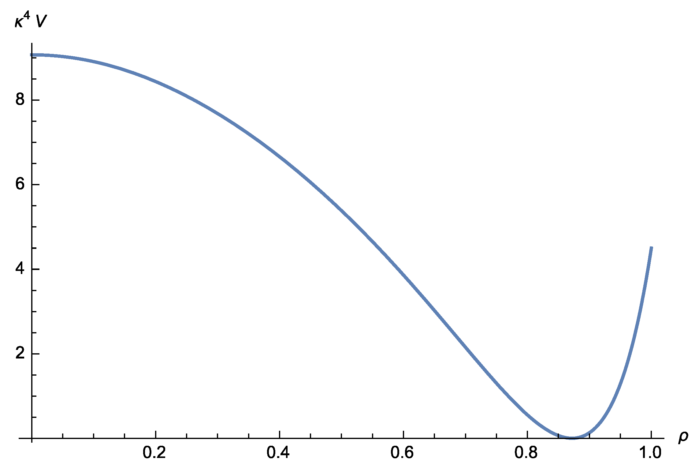
A plot of the potential for $A=1/2$, $q=1$, and f tuned so that the minimum has zero energy is given in Figure 1.

Note that, in this case, the superpotential is linear $W=fX$, describing the sgoldstino [33,34,35,36,37,38]. Indeed, modulo a D-term contribution, the inflaton in this model is the superpartner of the goldstino. In fact, for $q=0$ the inflaton reduces to the partner of the goldstino, as in Minimal Inflation models [39,40,41]. The important difference, however, is that this is a microscopic realisation of the identification of the inflaton with the sgoldstino, and the so-called $\eta$-problem is avoided (see discussion below).

The kinetic terms for the scalars can be written as 5

$$\begin{array}{ccc}\hfill {\mathcal{L}}_{\mathrm{kin}}& =& -g_{X\overline{X}}{\widehat{\partial }}_{\mu }X{\widehat{\partial }}^{\mu }X\hfill \\ & =& -g_{X\overline{X}}\left[{\partial }_{\mu }\rho {\partial }^{\mu }\rho +{\rho }^2\left({\partial }_{\mu }\theta +q{A}_{\mu }\right)\left({\partial }^{\mu }\theta +q{A}^{\mu }\right)\right].\hfill \end{array}$$

(19)

It was already anticipated above that the phase $\theta$ plays the role of the longitudinal component of the gauge field $A_{\mu }$, which acquires a mass by a Brout-Englert-Higgs mechanism.

We now interpret the field $\rho$ as the inflaton. It is important to emphasise that, in contrast with usual supersymmetric theories of inflation where one necessarily has two scalar degrees of freedom resulting in multifield inflation [42], our class of models contains only one scalar field $\rho$ as the inflaton. In order to calculate the slow-roll parameters, one needs to work with the canonically normalised field $\chi$ satisfying

$$\begin{array}{c}\hfill \frac{d\chi }{d\rho }=\sqrt{2g_{X\overline{X}}}.\end{array}$$

(20)

The slow-roll parameters are given in terms of the canonical field $\chi$ by

$$\begin{array}{c}\hfill ϵ=\frac{1}{2{\kappa }^2}{\left(\frac{dV/d\chi }{V}\right)}^2,\eta =\frac{1}{{\kappa }^2}\frac{d^{2}V/d{\chi }^2}{V}.\end{array}$$

(21)

Since we assume inflation to start near $\rho =0$, we expand

$$\begin{array}{cc}\hfill ϵ& =4{\left(\frac{-4A+x^2}{2+x^2}\right)}^2{\rho }^2+\mathcal{O}\left({\rho }^4\right),\\ \hfill \eta & =2\left(\frac{-4A+x^2}{2+x^2}\right)+\mathcal{O}\left({\rho }^2\right),\end{array}$$

(22)

where we defined $q=fx$. Notice that, for $\rho \ll 1$, the $ϵ$ parameter is very small, while the $\eta$ parameter can be made small by carefully tuning the parameter A. Any higher-order corrections to the Kähler potential do not contribute to the leading contributions in the expansion near $\rho =0$ for $\eta$ and $ϵ$. Such corrections can therefore be used to alter the potential near its minimum, at some point $X\ne 0$ without influencing the slow-roll parameters.

Note that there are two ways to evade the $\eta$-problem:

• First, one can obtain small $\eta$ by having a small $q\ll f$, while A should be of order $\mathcal{O}\left({10}^{-1}\right)$. In this case, the role of the gauge symmetry is merely to constrain the form of the Kähler potential and the superpotential, and to provide a Higgs mechanism which eliminates the extra scalar (phase) degree of freedom.
• Alternatively, there could be a cancellation between $q^2$ and $4A{f}^2$.

Since A is the second term in the expansion of the Kähler potential Equation (10), it is natural to be of order $\mathcal{O}\left({10}^{-1}\right)$ and therefore provides a solution to the $\eta$-problem.

4. On the New FI Term

4.1. Review

In [23], the authors proposed a new contribution to the supergravity Lagrangian of the form 6

$$\begin{array}{cc}\hfill {\mathcal{L}}_{\mathrm{FI}}& ={\xi }_2{\left[S_0{\overline{S}}_0\frac{w^2{\overline{w}}^2}{\overline{T}\left(w^2\right)T\left({\overline{w}}^2\right)}{\left(V\right)}_D\right]}_D.\hfill \end{array}$$

(23)

The chiral compensator field $S_0$, with Weyl and chiral weights $(\mathrm{Weyl}, \mathrm{Chiral})=(1,1)$, has components $S_0=\left(s_0,P_L{\Omega }_0,F_0\right)$. The vector multiplet has vanishing Weyl and chiral weights, and its components are given by $V=\left(v,\zeta ,\mathcal{H},v_{\mu },\lambda ,D\right)$. In the Wess-Zumino gauge, the first components are put to zero $v=\zeta =\mathcal{H}=0$. The multiplet $w^2$ is of weights $(1,1)$, and given by

$$\begin{array}{c}\hfill w^2=\frac{\overline{\lambda }{P}_L\lambda }{S_0^2},{\overline{w}}^2=\frac{\lambda P_R\overline{\lambda }}{{\overline{S}}_0^2}.\end{array}$$

(24)

The components of $\overline{\lambda }{P}_L\lambda$ are given by

$$\begin{array}{c}\hfill \overline{\lambda }{P}_L\lambda =\left(\overline{\lambda }{P}_L\lambda ;\sqrt{2}{P}_L\left(-\frac{1}{2}\gamma ·\widehat{F}+iD\right)\lambda ;2\overline{\lambda }{P}_L\mathcal{D}\lambda +{\widehat{F}}^{-}·{\widehat{F}}^{-}-D^2\right).\end{array}$$

(25)

The kinetic terms for the gauge multiplet are given by

$$\begin{array}{c}\hfill {\mathcal{L}}_{\mathrm{kin}}=-\frac{1}{4}{\left[\overline{\lambda }{P}_L\lambda \right]}_F+\mathrm{h}.\mathrm{c}..\end{array}$$

(26)

The operator T ($\overline{T}$) is defined in [44,45], and leads to a chiral (antichiral) multiplet. For example, the chiral multiplet $T\left({\overline{w}}^2\right)$ has weights $(2,2)$. In global supersymmetry the operator T corresponds to the usual chiral projection operator ${\overline{D}}^2$. 7

From now on, we will drop the notation of h.c., and implicitly assume its presence for every ${\left[\right]}_F$ term in the Lagrangian. Finally, the multiplet ${\left(V\right)}_D$ is a linear multiplet with weights $(2,0)$, given by

$$\begin{array}{c}\hfill {\left(V\right)}_D=\left(D,\mathcal{D}\lambda ,0,{\mathcal{D}}^b{\widehat{F}}_{ab},-\mathcal{D}\mathcal{D}\lambda ,-{\square }^{C}D\right).\end{array}$$

(27)

The definitions of $\mathcal{D}\lambda$ and the covariant field strength ${\widehat{F}}_{ab}$ can be found in Equation (17.1) of [28], which reduce, for an abelian gauge field, to

$$\begin{array}{cc}\hfill {\widehat{F}}_{ab}& =e_a^{\mu }{e}_b^{\nu }\left(2{\partial }_{[\mu }{A}_{\nu ]}+{\overline{\psi }}_{[\mu }{\gamma }_{\nu ]}\lambda \right)\hfill \\ \hfill {\mathcal{D}}_{\mu }\lambda & =\left({\partial }_{\mu }-\frac{3}{2}{b}_{\mu }+\frac{1}{4}{w}_{\mu }^{ab}{\gamma }_{ab}-\frac{3}{2}i{\gamma }_{\ast }{\mathcal{A}}_{\mu }\right)\lambda -\left(\frac{1}{4}{\gamma }^{ab}{\widehat{F}}_{ab}+\frac{1}{2}i{\gamma }_{\ast }D\right){\psi }_{\mu }.\hfill \end{array}$$

(28)

Here, $e_a^{\mu }$ is the vierbein, with frame indices $a,b$ and coordinate indices $\mu ,\nu$. The fields $w_{\mu }^{ab}$, $b_{\mu }$, and ${\mathcal{A}}_{\mu }$ are the gauge fields corresponding to Lorentz transformations, dilatations, and $T_R$ symmetry of the conformal algebra respectively, while ${\psi }_{\mu }$ is the gravitino. The conformal d’Alembertian is given by ${\square }^C={\eta }^{ab}{\mathcal{D}}_a{\mathcal{D}}_b$.

It is important to note that the FI term given by Equation (23) does not require the gauging of an R-symmetry, but breaks invariance under Kähler transformations. In fact, a gauged R-symmetry would forbid such a term ${\mathcal{L}}_{FI}$ [23]. 8

The resulting Lagrangian, after integrating out the auxiliary field D, contains a term

$$\begin{array}{c}\hfill {\mathcal{L}}_{\mathrm{FI},\mathrm{new}}=-\frac{{\xi }_2^2}{2}{\left(s_0{\overline{s}}_0\right)}^2.\end{array}$$

(29)

In the absence of additional matter fields, one can use the Poincaré gauge $s_0={\overline{s}}_0=1$, resulting in a constant D-term contribution to the scalar potential. This prefactor, however, is relevant when matter couplings are included in the next section.

4.2. Adding (Charged) Matter Fields

In this section, we couple the term ${\mathcal{L}}_{\mathrm{FI}}$ given by Equation (23) to additional matter fields charged under the $U\left(1\right)$. For simplicity, we focus on a single chiral multiplet X; the extension to more chiral multiplets is trivial. The Lagrangian is given by

$$\begin{array}{c}\hfill \mathcal{L}=-3{\left[S_0{\overline{S}}_0{e}^{-\frac{1}{3}K(X,\overline{X})}\right]}_D+{\left[S_0^{3}W\left(X\right)\right]}_F-\frac{1}{4}{\left[f\left(X\right)\overline{\lambda }{P}_L\lambda \right]}_F+{\mathcal{L}}_{\mathrm{FI}},\end{array}$$

(30)

with a Kähler potential $K(X,\overline{X})$, a superpotential $W\left(X\right)$, and a gauge kinetic function $f\left(X\right)$. The first three terms in Equation (30) give the usual supergravity Lagrangian [28]. We assume that the multiplet X transforms under the $U\left(1\right)$,

$$\begin{array}{cc}\hfill V& \to V+\Lambda +\overline{\Lambda },\hfill \\ \hfill X& \to X{e}^{-q\Lambda },\hfill \end{array}$$

(31)

with gauge multiplet parameter $\Lambda$. We assume that the $U\left(1\right)$ is not an R-symmetry. In other words, we assume that the superpotential does not transform under the gauge symmetry. For a model with a single chiral multiplet, this implies that the superpotential is constant

$$\begin{array}{c}\hfill W\left(X\right)=F.\end{array}$$

(32)

Gauge invariance fixes the Kähler potential to be a function of $X{e}^{qV}\overline{X}$ (for notational simplicity, in the following we omit the $e^{qV}$ factors).

Indeed, in this case, the term ${\mathcal{L}}_{\mathrm{FI}}$ can be consistently added to the theory, similar to [23], and the resulting D-term contribution to the scalar potential acquires an extra term proportional to ${\xi }_2$

$$\begin{array}{cc}\hfill {\mathcal{V}}_D& =\frac{1}{2}\mathrm{Re}{\left(f\left(X\right)\right)}^{-1}{\left(i{k}_X{\partial }_{X}K+{\xi }_2{e}^{\frac{2}{3}K}\right)}^2,\hfill \end{array}$$

(33)

where the Killing vector is $k_X=-iqX$ and $f\left(X\right)$ is the gauge kinetic function. The F-term contribution to the scalar potential remains the usual

$$\begin{array}{cc}\hfill {\mathcal{V}}_F& =e^{K(X,\overline{X})}\left(-3W\overline{W}+g^{X\overline{X}}{\nabla }_{X}W{\overline{\nabla }}_{\overline{X}}\overline{W}\right).\hfill \end{array}$$

(34)

For a constant superpotential (32), this reduces to

$$\begin{array}{cc}\hfill {\mathcal{V}}_F& ={\left|F\right|}^2{e}^{K(X,\overline{X})}\left(-3+g^{X\overline{X}}{\partial }_{X}K{\partial }_{\overline{X}}K\right).\hfill \end{array}$$

(35)

From Equation (33) it can be seen that, if the Kähler potential includes a term proportional to ${\xi }_{1}log\left(X\overline{X}\right)$, the D-term contribution to the scalar potential acquires another constant contribution. For example, if

$$\begin{array}{c}\hfill K(X,\overline{X})=X\overline{X}+{\xi }_{1}ln\left(X\overline{X}\right),\end{array}$$

(36)

the D-term contribution to the scalar potential becomes

$$\begin{array}{cc}\hfill {\mathcal{V}}_D& =\frac{1}{2}\mathrm{Re}{\left(f\left(X\right)\right)}^{-1}{\left(qX\overline{X}+q{\xi }_1+{\xi }_2{e}^{\frac{2}{3}K}\right)}^2.\hfill \end{array}$$

(37)

In fact, the contribution proportional to ${\xi }_1$ is the usual FI term in a non R-symmetric Kähler frame, which can be consistently added to the model including the new FI term proportional to ${\xi }_2$.

In the absence of the extra term, a Kähler transformation

$$\begin{array}{cc}\hfill K(X,\overline{X})& \to K(X,\overline{X})+J\left(X\right)+\overline{J}\left(\overline{X}\right),\hfill \\ \hfill W\left(X\right)& \to W\left(X\right)e^{-J\left(X\right)},\hfill \end{array}$$

(38)

with $J\left(X\right)=-{\xi }_{1}lnX$ allows one to recast the model in the form

$$\begin{array}{cc}\hfill K(X,\overline{X})& =X\overline{X},\hfill \\ \hfill W\left(X\right)& =m_{3/2}X.\hfill \end{array}$$

(39)

The two models result in the same Lagrangian, at least classically 9. However, in the Kähler frame of Equations (39), the superpotential transforms nontrivially under the gauge symmetry. As a consequence, the gauge symmetry becomes an R-symmetry. Note that [24]:

• The extra term (23) violates the Kähler invariance of the theory, and the two models related by a Kähler transformation are no longer equivalent.
• The model written in the Kähler frame where the gauge symmetry becomes an R-symmetry in Equations (39) can not be consistently coupled to ${\mathcal{L}}_{\mathrm{FI}}$.

5. The Scalar Potential in a Non R-Symmetry Frame

In this section, we work in the Kähler frame where the superpotential does not transform, and take into account the two types of FI terms which were discussed in the last section. For convenience, we repeat here the Kähler potential in Equation (36) and restore the inverse reduced Planck mass $\kappa =M_{\mathrm{Pl}}^{-1}={(2.4\times {10}^{18}\mathrm{GeV})}^{-1}$:

$$K={\kappa }^{-2}(X\overline{X}+{\xi }_{1}lnX\overline{X}).$$

(40)

The superpotential and the gauge kinetic function are set to be constant 10:

$$W={\kappa }^{-3}F,f\left(X\right)=1.$$

(41)

After performing a change of the field variable $X=\rho e^{i\theta }$, where $\rho \ge 0$ and setting ${\xi }_1=b$, the full scalar potential $\mathcal{V}={\mathcal{V}}_F+{\mathcal{V}}_D$ is a function of $\rho$. The F-term contribution to the scalar potential is given by

$${\mathcal{V}}_F=\frac{1}{{\kappa }^4}{F}^2{e}^{{\rho }^2}{\rho }^{2b}\left[\frac{{\left(b+{\rho }^2\right)}^2}{{\rho }^2}-3\right],$$

(42)

and the D-term contribution is

$${\mathcal{V}}_D=\frac{q^2}{2{\kappa }^4}{\left(b+{\rho }^2+\xi {\rho }^{\frac{4b}{3}}{e}^{\frac{2}{3}{\rho }^2}\right)}^2.$$

(43)

Note that we rescaled the second FI parameter by $\xi ={\xi }_2/q$. We consider the case with $\xi \ne 0$, as we are interested in the role of the new FI-term in inflationary models driven by supersymmetry breaking. Moreover, the limit $\xi \to 0$ is ill-defined [23].

The first FI parameter b was introduced as a free parameter. We now proceed to narrowing the value of b by the following physical requirements. We first consider the behaviour of the potential around $\rho =0$,

$$\begin{array}{cc}\hfill {\mathcal{V}}_D& =\frac{q^2}{2{\kappa }^4}\left[\left(b^2+2b{\rho }^2+O\left({\rho }^4\right)\right)+2b\xi {\rho }^{\frac{4b}{3}}\left(1+O\left({\rho }^2\right)\right)+{\xi }^2{\rho }^{\frac{8b}{3}}\left(1+O\left({\rho }^2\right)\right)\right],\hfill \end{array}$$

(44)

$$\begin{array}{cc}\hfill {\mathcal{V}}_F& =\frac{F^2}{{\kappa }^4}{\rho }^{2b}\left[b^2{\rho }^{-2}+(2b-3)+O\left({\rho }^2\right)\right].\hfill \end{array}$$

(45)

Here we are interested in small-field inflation models, in which the inflation starts in the neighbourhood of a local maximum at $\rho =0$. In [21], we considered models of this type with $\xi =0$ (which were called Case 1 models), and found that the choice $b=1$ is forced by the requirement that the potential takes a finite value at the local maximum $\rho =0$. Now, we will investigate the effect of the new FI parameter $\xi$ on the choice of b under the same requirement.

First, in order for $\mathcal{V}\left(0\right)$ to be finite, we need $b\ge 0$. We first consider the case $b>0$. We next investigate the condition that the potential at $\rho =0$ has a local maximum. For clarity, we discuss below the cases of $F=0$ and $F\ne 0$ separately. The $b=0$ case will be treated at the end of this section.

5.1. Case $F=0$

In this case, ${\mathcal{V}}_F=0$ and the scalar potential is given by only the D-term contribution $\mathcal{V}={\mathcal{V}}_D$. Let us first discuss the first derivative of the potential:

$$\begin{array}{c}\hfill {\mathcal{V}}_D^{\prime }=\frac{q^2}{2{\kappa }^4}\left[4b\rho \left(1+O\left({\rho }^2\right)\right)+\frac{8b^2}{3}\xi {\rho }^{\frac{4b}{3}-1}\left(1+O\left({\rho }^2\right)\right)+\frac{8b}{3}{\xi }^2{\rho }^{\frac{8b}{3}-1}\left(1+O\left({\rho }^2\right)\right)\right].\end{array}$$

(46)

For ${\mathcal{V}}_D^{\prime }\left(0\right)$ to be convergent, we need $b\ge 3/4$ (note that $\xi \ne 0$). When $b=3/4$, we have ${\mathcal{V}}_D^{\prime }\left(0\right)=8b^2\xi /3$, which does not give an extremum as we chose $\xi \ne 0$. On the other hand, when $b>3/4$, we have ${\mathcal{V}}_D^{\prime }\left(0\right)=0$. To narrow the allowed value of b further, let us turn to the second derivative,

$$\begin{array}{cc}\hfill {\mathcal{V}}_D^{″}& =\frac{q^2}{2{\kappa }^4}[4b\left(1+O\left({\rho }^2\right)\right)+\frac{8b^2}{3}\left(\frac{4b}{3}-1\right)\xi {\rho }^{\frac{4b}{3}-2}\left(1+O\left({\rho }^2\right)\right)\hfill \\ & +\frac{8b}{3}\left(\frac{8b}{3}-1\right){\xi }^2{\rho }^{\frac{8b}{3}-2}\left(1+O\left({\rho }^2\right)\right)].\hfill \end{array}$$

(47)

When $3/4<b<3/2$, the second derivative ${\mathcal{V}}_D^{″}\left(0\right)$ diverges. When $b>3/2$, the second derivative becomes ${\mathcal{V}}_D^{″}\left(0\right)=2{\kappa }^{-4}{q}^{2}b>0$, which gives a minimum.

We therefore conclude that to have a local maximum at $\rho =0$, we need to choose $b=3/2$, for which we have

$$\begin{array}{c}\hfill {\mathcal{V}}_D^{″}\left(0\right)=3{\kappa }^{-4}{q}^2(\xi +1).\end{array}$$

(48)

the condition that $\rho =0$ is a local maximum requires $\xi <-1$.

Let us next discuss the global minimum of the potential with $b=3/2$ and $\xi <-1$. The first derivative of the potential without approximation reads

$$\begin{array}{c}\hfill {\mathcal{V}}_D^{\prime }\propto \rho (3+3\xi e^{\frac{2}{3}{\rho }^2}+2\xi {\rho }^2{e}^{\frac{2}{3}{\rho }^2})(3+2{\rho }^2+2\xi {\rho }^2{e}^{\frac{2}{3}{\rho }^2}).\end{array}$$

(49)

Since $3+3\xi e^{\frac{2}{3}{\rho }^2}+2\xi {\rho }^2{e}^{\frac{2}{3}{\rho }^2}<0$ for $\rho \ge 0$ and $\xi <-1$, the extremum away from $\rho =0$ is located at ${\rho }_v$ satisfying the condition

$$\begin{array}{c}\hfill 3+2{\rho }_v^2+2\xi {\rho }_v^2{e}^{\frac{2}{3}{\rho }_v^2}=0.\end{array}$$

(50)

Substituting this condition into the potential ${\mathcal{V}}_D$ gives ${\mathcal{V}}_D\left({\rho }_v\right)=0$.

We conclude that, for $\xi <-1$ and $b=3/2$, the potential has a maximum at $\rho =0$, and a supersymmetric minimum at ${\rho }_v$. We postpone the analysis of inflation near the maximum of the potential to Section 6, and the discussion of the uplifting of the minimum, in order to obtain a small but positive cosmological constant below. In the next subsection, we investigate the case $F\ne 0$.

We finally comment on supersymmetry breaking in the scalar potential. Since the superpotential is zero, the SUSY breaking is measured by the D-term order parameter, namely the Killing potential associated with the gauged $\mathrm{U}\left(1\right)$, which is defined by

$$\begin{array}{cc}\hfill \mathcal{D}& =i{\kappa }^{-2}\frac{-iqX}{W}\left(\frac{\partial W}{\partial X}+{\kappa }^2\frac{\partial \mathcal{K}}{\partial X}W\right).\hfill \end{array}$$

(51)

This enters the scalar potential as ${\mathcal{V}}_D={\mathcal{D}}^2/2$. So, at the local maximum and during inflation, $\mathcal{D}$ is of order q and supersymmetry is broken. On the other hand, at the global minimum, supersymmetry is preserved and the potential vanishes.

5.2. Case $F\ne 0$

In this section, we take into account the effect of ${\mathcal{V}}_F$; its first derivative reads:

$$\begin{array}{cc}\hfill {\mathcal{V}}_F^{\prime }& ={\kappa }^{-4}{F}^2\left[b^2(2b-2){\rho }^{2b-3}+2b(2b-3){\rho }^{2b-1}\left(1+O\left({\rho }^2\right)\right)\right].\hfill \end{array}$$

(52)

For ${\mathcal{V}}^{\prime }\left(0\right)$ to be convergent, we need $b\ge 3/2$, for which ${\mathcal{V}}_D^{\prime }\left(0\right)=0$ holds. For $b=3/2$, we have ${\mathcal{V}}_F^{\prime }\left(0\right)=(9/4){\kappa }^{-4}{F}^2>0$, which does not give an extremum. For $b>3/2$, we have ${\mathcal{V}}_F^{\prime }\left(0\right)=0$. To narrow the allowed values of b further, let us turn to the second derivative:

$$\begin{array}{cc}\hfill {\mathcal{V}}_F^{″}& ={\kappa }^{-4}{F}^2\left[b^2(2b-2)(2b-3){\rho }^{2b-4}+2b(2b-3)(2b-1){\rho }^{2b-2}\left(1+O\left({\rho }^2\right)\right)\right].\hfill \end{array}$$

(53)

For $3/2<b<2$, the second derivative ${\mathcal{V}}_F^{″}\left(0\right)$ diverges. For $b\ge 2$, the second derivative is positive ${\mathcal{V}}^{″}\left(0\right)>0$, which gives a minimum (note that $V_D^{″}\left(0\right)>0$ as well in this range).

We conclude that the potential cannot have a local maximum at $\rho =0$ for any choice of b. Nevertheless, as we will show below, the potential can have a local maximum in the neighbourhood of $\rho =0$ if we choose $b=3/2$ and $\xi <-1$. For this choice, the derivatives of the potential have the following properties:

$$\begin{array}{c}\hfill {\mathcal{V}}^{\prime }\left(0\right)<0,{\mathcal{V}}^{″}\left(0\right)=3{\kappa }^{-4}{q}^2(\xi +1).\end{array}$$

(54)

The extremisation condition around $\rho =0$ becomes

$$\begin{array}{c}\hfill 3{\kappa }^{-4}{q}^2(\xi +1)\rho +\frac{9}{4}{\kappa }^{-4}{F}^2\simeq 0.\end{array}$$

(55)

So, the extremum is at

$$\begin{array}{c}\hfill \rho \simeq -\frac{3F^2}{4q^2(\xi +1)}.\end{array}$$

(56)

Note that the extremum is in the neighbourhood of $\rho =0$, as long as we keep the F-contribution to the scalar potential small by taking $F^2\ll q^2|\xi +1|$, which guarantees the approximation-ignoring higher order terms in $\rho$. We now choose $\xi <-1$, so that $\rho$ for this extremum is positive. The second derivative at the extremum reads

$$\begin{array}{c}\hfill {\mathcal{V}}^{″}\simeq 3{\kappa }^{-4}{q}^2(\xi +1),\end{array}$$

(57)

as long as we ignore the higher order terms in $F^2/(q^2|\xi +1|)$. By our choice $\xi <-1$, the extremum is a local maximum, as desired.

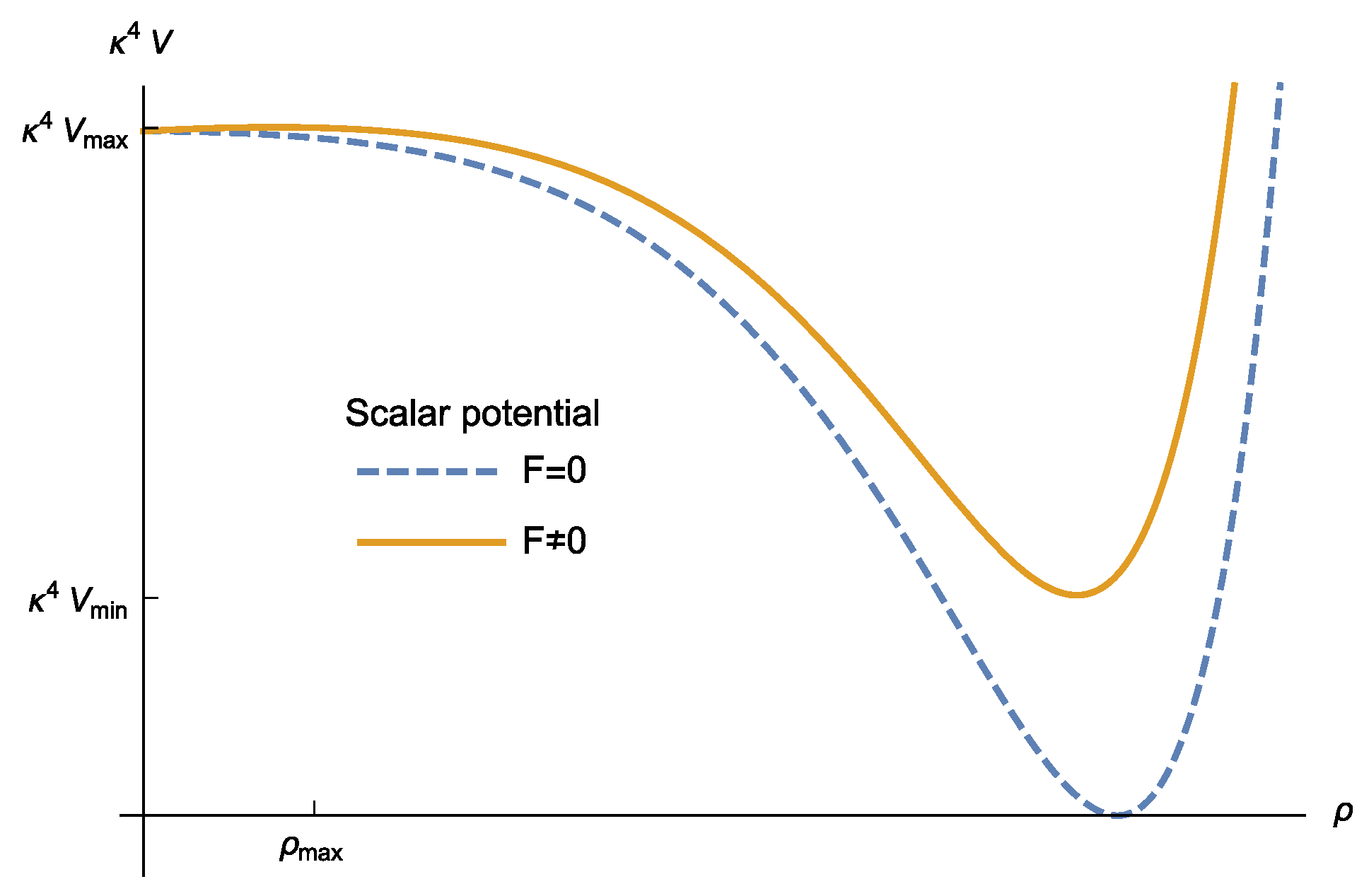
Let us comment on the global minimum after turning on the F-term contribution. As long as we choose the parameters so that $F^2/q^2\ll 1$, the change in the global minimum ${\rho }_v$ is very small (of order $\mathcal{O}(F^2/q^2)$), because the extremisation condition depends only on the ratio $F^2/q^2$. So, the change in the value of the global minimum is of order $\mathcal{O}\left(F^2\right)$. The plot of this change is given in Figure 2.

In the present case $F\ne 0$, the order parameters of SUSY breaking are both the Killing potential $\mathcal{D}$ and the F-term contribution ${\mathcal{F}}_X$, which read

$$\begin{array}{cc}\hfill \mathcal{D}& \propto q(\frac{3}{2}+{\rho }^2),{\mathcal{F}}_X\propto F{\rho }^{1/2}{e}^{{\rho }^2/2},\hfill \end{array}$$

(58)

where the F-term order parameter ${\mathcal{F}}_X$ is defined by

$$\begin{array}{cc}\hfill {\mathcal{F}}_X& =-\frac{1}{\sqrt{2}}{e}^{{\kappa }^2\mathcal{K}/2}{\left(\frac{{\partial }^2\mathcal{K}}{\partial X\partial \overline{X}}\right)}^{-1}\left(\frac{\partial \overline{W}}{\partial \overline{X}}+{\kappa }^2\frac{\partial \mathcal{K}}{\partial \overline{X}}\overline{W}\right).\hfill \end{array}$$

(59)

therefore, at the local maximum, ${\mathcal{F}}_X/\mathcal{D}$ is of order $\mathcal{O}({(\xi +1)}^{-1/2}{F}^2/q^2)$ because $\rho$ at that point is of order $\mathcal{O}({(\xi +1)}^{-1}{F}^2/q^2)$. On the other hand, at the global minimum, both $\mathcal{D}$ and ${\mathcal{F}}_X$ are of order $\mathcal{O}\left(F\right)$, assuming that $\rho$ at the minimum is of order $\mathcal{O}\left(1\right)$, which is true in our models below. This makes tuning of the vacuum energy between the F- and D-contribution, in principle, possible, along the lines of [10,21].

A comment must be made here on the action in the presence of non-vanishing F and $\xi$. As mentioned above, the supersymmetry is broken both by the gauge sector and by the matter sector. The associated goldstino therefore consists of a linear combination of the $U\left(1\right)$ gaugino and the fermion in the matter chiral multiplet X. In the unitary gauge the goldstino is set to zero, so the gaugino is not vanishing and the action does not simplify as in Ref. [23]. This, however, only affects the part of the action with fermions, while the scalar potential does not change. This is why we nevertheless used the scalar potential (42) and (43).

Let us consider the case $b=0$, where only the new FI parameter $\xi$ contributes to the potential. In this case, the condition for the local maximum of the scalar potential at $\rho =0$ can be satisfied for $-\frac{3}{2}<\xi <0$. When F is set to zero, the scalar potential (43) has a minimum at ${\rho }_{\min }^2=\frac{3}{2}ln\left(-\frac{3}{2\xi }\right)$. In order to have ${\mathcal{V}}_{\min }=0$, we can choose $\xi =-\frac{3}{2e}$. However, we find that this choice of parameter $\xi$ does not allow slow-roll inflation near the maximum of the scalar potential. Similar to the previous model of Section 3, it may be possible to achieve both the scalar potential satisfying slow-roll conditions and a small cosmological constant at the minimum, by adding correction terms to the Kähler potential and turning on a parameter F. However, here, we will focus on the $b=3/2$ case where, as we will see shortly, less parameters are required to satisfy the observational constraints.

6. Application in Inflation

We recall that in the models we described in Section 3, the inflaton is identified with the sgoldstino, carrying a $U\left(1\right)$ charge under a gauged R-symmetry and inflation occurs around the maximum of the scalar potential, where the $U\left(1\right)$ symmetry is restored, with the inflaton rolling down towards the electroweak minimum. These models avoid the so-called $\eta$-problem in supergravity by taking a linear superpotential, $W\propto X$. In contrast, here we will consider models with two FI parameters $b,\xi$ in the Kähler frame, where the $U\left(1\right)$ gauge symmetry is not an R-symmetry. If the new FI term $\xi$ is zero, these models are Kähler equivalent to those with a linear superpotential (Case 1 models with $b=1$). The presence of non-vanishing $\xi$, however, breaks the Kähler invariance (as discussed above). Moreover, the FI parameter b cannot be 1, but is forced to be $b=3/2$, according to the argument in Section 5. So, the new models do not seem to avoid the $\eta$-problem. Nevertheless, we will show below that this is not the case, and the new models with $b=3/2$ avoid the $\eta$-problem thanks to the other FI parameter $\xi$—which is chosen near the value at which the effective charge of X vanishes between the two FI-terms. Inflation is again driven from supersymmetry breaking, but from a D-term rather than an F-term as we had before.

6.1. Example for Slow-Roll D-Term Inflation

In this section, we focus on the case where $b=3/2$ and derive the condition that leads to slow-roll inflation scenarios, where the start of inflation (or, horizon crossing) is near the maximum of the potential, at $\rho =0$. We also assume that the scalar potential is D-term dominated by choosing $F=0$, for which the model has only two parameters, namely q and $\xi$. The parameter q controls the overall scale of the potential, and will be fixed by the amplitude $A_s$ of the CMB data. The only free parameter left over is $\xi$, which can be tuned to satisfy the slow-roll condition.

In order to calculate the slow-roll parameters, we need to work with the canonically normalised field $\chi$ defined by Equations (20) and (21). Since we assume inflation to start near $\rho =0$, the slow-roll parameters for small $\rho$ can be expanded as

$$\begin{array}{cc}\hfill ϵ& =\frac{F^4}{q^4}+\frac{4F^2\left(2(\xi +1)q^4-3F^4\right)}{3q^6}\rho \hfill \\ & +\left(\frac{16}{9}{(\xi +1)}^2+\frac{2F^4\left(18F^4-q^4(20\xi +11)\right)}{3q^8}\right){\rho }^2+\mathcal{O}\left({\rho }^3\right),\hfill \\ \hfill \eta & =\frac{4(1+\xi )}{3}+\mathcal{O}\left(\rho \right).\hfill \end{array}$$

(60)

Note that $\eta$ is negative when $\xi <-1$. We can, therefore, tune the parameter $\xi$ to avoid the $\eta$-problem. The observation is that at $\xi =-1$, the effective charge of X vanishes and thus the $\rho$-dependence in the D-term contribution (43) becomes of quartic order.

For our present choice $F=0$, the potential and the slow-roll parameters become functions of ${\rho }^2$ and the slow-roll parameters for small ${\rho }^2$ read

$$\begin{array}{cc}\hfill \eta & =\frac{4(1+\xi )}{3}+\mathcal{O}\left({\rho }^2\right),\hfill \\ \hfill ϵ& =\frac{16}{9}{(\xi +1)}^2{\rho }^2+\mathcal{O}\left({\rho }^4\right)\simeq \eta {\left(0\right)}^2{\rho }^2.\hfill \end{array}$$

(61)

Note that we obtain the same relation between $ϵ$ and $\eta$ as in the model of inflation from supersymmetry breaking, driven by an F-term from a linear superpotential and $b=1$ (see Equation (22)). Thus, there is a possibility to have a flat plateau near the maximum that satisfies the slow-roll condition and at the same time a small cosmological constant at the minimum nearby.

The number of e-folds N during inflation is determined by

$$\begin{array}{c}\hfill N={\kappa }^2{\int }_{{\chi }_{\ast }}^{{\chi }_{\mathrm{end}}}\frac{\mathcal{V}}{{\partial }_{\chi }\mathcal{V}}d\chi ={\kappa }^2{\int }_{{\rho }_{\ast }}^{{\rho }_{\mathrm{end}}}\frac{\mathcal{V}}{{\partial }_{\rho }\mathcal{V}}{\left(\frac{d\chi }{d\rho }\right)}^{2}d\rho ,\end{array}$$

(62)

where we choose $\left|ϵ\right({\chi }_{\mathrm{end}}\left)\right|=1$. Notice that the slow-roll parameters for small ${\rho }^2$ satisfy the simple relation $ϵ=\eta {\left(0\right)}^2{\rho }^2+O\left({\rho }^4\right)$ by Equation (61). Therefore, the number of e-folds between $\rho ={\rho }_1$ and ${\rho }_2$ (${\rho }_1<{\rho }_2$) takes the following simple approximate form, exactly as in the previous model of F-term inflation described in Section 3.

$$\begin{array}{c}\hfill N\simeq \frac{1}{\left|\eta \right(0\left)\right|}ln\left(\frac{{\rho }_2}{{\rho }_1}\right)=\frac{3}{4|\xi +1|}ln\left(\frac{{\rho }_2}{{\rho }_1}\right),\end{array}$$

(63)

as long as the expansions in (61) are valid in the region ${\rho }_1\le \rho \le {\rho }_2$. Here, we also used the approximation $\eta \left(0\right)\simeq {\eta }_{\ast }$, which holds in this approximation.

We can compare the theoretical predictions of our model to the observational data, via the power spectrum of scalar perturbations of the CMB, namely the amplitude $A_s$, tilt $n_s$, and the tensor-to-scalar ratio of primordial fluctuations r. These are written in terms of the slow-roll parameters:

$$\begin{array}{cc}\hfill A_s& =\frac{{\kappa }^4{\mathcal{V}}_{\ast }}{24{\pi }^2{ϵ}_{\ast }},\hfill \\ \hfill n_s& =1+2{\eta }_{\ast }-6{ϵ}_{\ast }\simeq 1+2{\eta }_{\ast },\hfill \\ \hfill r& =16{ϵ}_{\ast },\hfill \end{array}$$

(64)

where all parameters are evaluated by the field value at horizon crossing ${\chi }_{\ast }$. From the relation of the spectral index above, one should have ${\eta }_{\ast }\simeq -0.02$, and thus Equation (63) gives approximately the desired number of e-folds when the logarithm is of order one. Actually, using this formula, we can estimate the upper bound of the tensor-to-scalar ratio r and the Hubble scale $H_{\ast }$, following the same argument given in Section 3; that is, the upper bounds are given by computing the parameters $r,H_{\ast }$ assuming that the expansions (61) hold until the end of inflation. We then get the bound

$$\begin{array}{c}\hfill r\lesssim 16\left(\right|{\eta }_{\ast }{\left|{\rho }_{\mathrm{end}}{e}^{-|{\eta }_{\ast }|N}\right)}^2\simeq {10}^{-4},H_{\ast }\lesssim {10}^{12}\mathrm{GeV},\end{array}$$

(65)

where we used $|{\eta }_{\ast }|=0.02$, $N\simeq 50-60$, and ${\rho }_{\mathrm{end}}\lesssim 0.5$, which are consistent with our models. In the next subsection, we will present a model which gives a tensor-to-scalar ratio bigger than the upper bound above, by adding some perturbative corrections to the Kähler potential.

As an example, let us consider the case where

$$\begin{array}{c}\hfill q=4.544\times {10}^{-7},\xi =-1.005.\end{array}$$

(66)

By choosing the initial condition ${\rho }_{\ast }=0.055$ and ${\rho }_{\mathrm{end}}=0.403$, we obtain the results $N=58$, $n_s=0.9542$, $r=7.06\times {10}^{-6}$, and $A_s=2.2\times {10}^{-9}$, which are within the $2\sigma$-region of the Planck’15 data [24].

As was shown in Section 5.1, this model has a supersymmetric minimum with zero cosmological constant as F was chosen to be zero. One possible way to generate a non-zero cosmological constant at the minimum is to turn on the superpotential $W={\kappa }^{-3}F\ne 0$, as mentioned in Section 5.2. In this case, the scale of the cosmological constant is of order $\mathcal{O}\left(F^2\right)$. It would be interesting to find an inflationary model which has a minimum at a tiny tuneable vacuum energy with a supersymmetry breaking scale consistent with low energy particle physics.

6.2. A Small Field Inflation Model from Supergravity with Observable Tensor-To-Scalar Ratio

While the results in the previous example agree with the current limits on r set by Planck, supergravity models with higher r are of particular interest. In this section we show that our model can attain large r, at the price of introducing some additional terms in the Kähler potential. Let us consider the previous model with additional quadratic and cubic terms in $X\overline{X}$:

$$K={\kappa }^{-2}\left(X\overline{X}+A{\left(X\overline{X}\right)}^2+B{\left(X\overline{X}\right)}^3+blnX\overline{X}\right),$$

(67)

while the superpotential and the gauge kinetic function remain as in Equation (41). We now assume that inflation is driven by the D-term, setting the parameter $F=0$. In terms of the field variable $\rho$, we obtain the scalar potential:

$$\mathcal{V}=q^2{\left(b+{\rho }^2+2A{\rho }^4+3B{\rho }^6+\xi {\rho }^{\frac{4b}{3}}{e}^{\frac{2}{3}\left(A{\rho }^4+B{\rho }^6+{\rho }^2\right)}\right)}^2.$$

(68)

We, thus, have two more parameters A and B. This does not affect the arguments of the choices of b in the previous sections, because these parameters appear in higher orders in $\rho$ in the scalar potential. So, we consider the case $b=3/2$. The simple formula (63) for the number of e-folds for small ${\rho }^2$ also holds, even when $A,B$ are turned on, because the new parameters appear at order ${\rho }^4$ and higher. To obtain $r\approx 0.01$, we can choose, for example,

$$\begin{array}{c}\hfill q=2.121\times {10}^{-5},\xi =-1.140,A=0.545,B=0.230.\end{array}$$

(69)

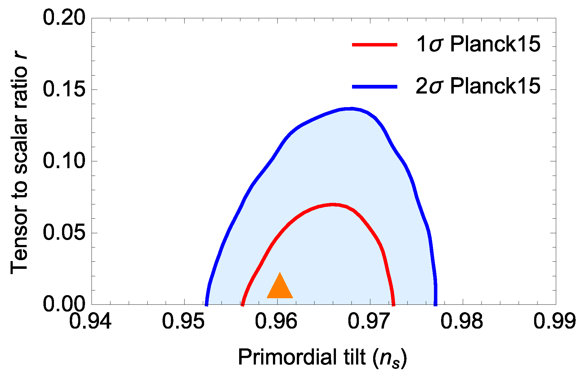
By choosing the initial condition ${\rho }_{\ast }=0.240$ and ${\rho }_{\mathrm{end}}=0.720$, we obtain the results $N=57$, $n_s=0.9603$, $r=0.015$, and $A_s=2.2\times {10}^{-9}$, which agree with the Planck’15 data, as shown in Figure 3.

In summary, in contrast to the model in Section 3, where the F-term contribution is dominant during inflation, here inflation is driven purely by a D-term. Moreover, a canonical Kähler potential (40) together with two FI-parameters (q and $\xi$) is enough to satisfy the Planck’15 constraints, and no higher-order correction to the Kähler potential is needed. However, to obtain a larger tensor-to-scalar ratio, we have to introduce perturbative corrections to the Kähler potential, up to cubic order in $X\overline{X}$ (i.e., up to order ${\rho }^6$). This model provides a supersymmetric extension of the model [47], which realises large r at small field inflation, without referring to supersymmetry.

References

- Antoniadis, I.; Knoops, R. Gauge R-symmetry and de Sitter vacua in supergravity and string theory. Nucl. Phys. B 2014, 86, 43–62. [Google Scholar] [CrossRef]
- Villadoro, G.; Zwirner, F. De Sitter Vacua via Consistent D Terms. Phys. Rev. Lett. 2005, 95, 231602. [Google Scholar] [CrossRef] [PubMed]
- Fayet, P.; Iliopoulos, J. Spontaneously Broken Supergauge Symmetries and Goldstone Spinors. Phys. Lett. B 1974, 51, 461–464. [Google Scholar] [CrossRef]
- Fayet, P. Spontaneously broken supersymmetric theories of weak, electromagnetic and strong interactions. Phys. Lett. B 1977, 69, 489–494. [Google Scholar] [CrossRef]
- Antoniadis, I.; Ghilencea, D.M.; Knoops, R. Gauged R-symmetry and its anomalies in 4D N = 1 supergravity and phenomenological implications. J. High Energy Phys. 2015, 2015, 166. [Google Scholar] [CrossRef]
- Antoniadis, I.; Knoops, R. MSSM soft terms from supergravity with gauged R-symmetry in de Sitter vacuum. Nucl. Phys. B 2016, 902, 69–94. [Google Scholar] [CrossRef] [Green Version]
- Antoniadis, I.; Maillard, T. Moduli stabilization from magnetic fluxes in type I string theory. Nucl. Phys. B 2005, 716, 3–32. [Google Scholar] [CrossRef] [Green Version]
- Antoniadis, I.; Kumar, A.; Maillard, T. Magnetic fluxes and moduli stabilization. Nucl. Phys. B 2007, 767, 139–162. [Google Scholar] [CrossRef] [Green Version]
- Antoniadis, I.; Derendinger, J.-P.; Maillard, T. Nonlinear N = 2 Supersymmetry, Effective Actions and Moduli Stabilization. Nucl. Phys. B 2009, 808, 53–79. [Google Scholar] [CrossRef]
- Antoniadis, I.; Chatrabhuti, A.; Sono, H.; Knoops, R. Inflation from Supergravity with Gauged R-symmetry in de Sitter Vacuum. Eur. Phys. J. C 2016, 76, 680. [Google Scholar] [CrossRef]
- Guth, A.H. The Inflationary Universe: A Possible Solution to the Horizon and Flatness Problems. Phys. Rev. D 1981, 23, 347. [Google Scholar] [CrossRef]
- Linde, A.D. A New Inflationary Universe Scenario: A Possible Solution of the Horizon, Flatness, Homogeneity, Isotropy and Primordial Monopole Problems. Phys. Lett. B 1982, 108, 389–393. [Google Scholar] [CrossRef]
- Albrecht, A.; Steinhardt, P.J. Cosmology for Grand Unified Theories with Radiatively Induced Symmetry Breaking. Phys. Rev. Lett. 1982, 48, 1220–1223. [Google Scholar] [CrossRef]
- Lyth, D.H.; Riotto, A. Particle physics models of inflation and the cosmological density perturbation. Phys. Rep. 1999, 314, 1–146. [Google Scholar] [CrossRef] [Green Version]
- Linde, A.D. Particle physics and inflationary cosmology. Contemp. Concepts Phys. 1990, 5, 1. [Google Scholar]
- Starobinsky, A.A. A New Type of Isotropic Cosmological Models Without Singularity. Phys. Lett. B 1980, 91, 99–102. [Google Scholar] [CrossRef]
- Randall, L.; Thomas, S.D. Solving the cosmological moduli problem with weak scale inflation. Nucl. Phys. B 1995, 449, 229–247. [Google Scholar] [CrossRef] [Green Version]
- Riotto, A. Inflation and the nature of supersymmetry breaking. Nucl. Phys. B 1998, 515, 413–435. [Google Scholar] [CrossRef] [Green Version]
- Izawa, K.I. Supersymmetry—Breaking models of inflation. Prog. Theor. Phys. 1998, 99, 157–159. [Google Scholar] [CrossRef]
- Buchmuller, W.; Covi, L.; Delepine, D. Inflation and supersymmetry breaking. Phys. Lett. B 2000, 491, 183. [Google Scholar] [CrossRef]
- Antoniadis, I.; Chatrabhuti, A.; Isono, H.; Knoops, R. Inflation from Supersymmetry Breaking. Eur. Phys. J. C 2017, 77, 724. [Google Scholar] [CrossRef]
- Catino, F.; Villadoro, G.; Zwirner, F. On Fayet-Iliopoulos terms and de Sitter vacua in supergravity: Some easy pieces. J. High Energy Phys. 2012, 2012, 2. [Google Scholar] [CrossRef]
- Cribiori, N.; Farakos, F.; Tournoy, M.; Van Proeyen, A. Fayet-Iliopoulos terms in supergravity without gauged R-symmetry. arXiv, 2017; arXiv:1712.08601. [Google Scholar] [CrossRef]
- Antoniadis, I.; Chatrabhuti, A.; Isono, H.; Knoops, R. Fayet-Iliopoulos terms in supergravity and D-term inflation. Eur. Phys. J. C 2018, 78, 366. [Google Scholar] [CrossRef]
- Aldabergenov, Y.; Ketov, S.V. Removing instability of inflation in Polonyi-Starobinsky supergravity by adding FI term. Mod. Phys. Lett. A 2018, 91, 1850032. [Google Scholar] [CrossRef]
- Ijjas, A.; Steinhardt, P.J.; Loeb, A. Inflationary paradigm in trouble after Planck2013. Phys. Lett. B 2013, 723, 261–266. [Google Scholar] [CrossRef] [Green Version]
- Antoniadis, I. Inflation from supersymmetry breaking. Int. J. Mod. Phys. A 2018, 33, 1844021. [Google Scholar] [CrossRef]
- Freedman, D.Z.; Van Proeyen, A. Supergravity; Cambridge University Press: Cambridge, UK, 2012. [Google Scholar]
- Schmitz, K.; Yanagida, T.T. Dynamical supersymmetry breaking and late-time R symmetry breaking as the origin of cosmic inflation. Phys. Rev. D 2016, 94, 074021. [Google Scholar] [CrossRef]
- Binetruy, P.; Dvali, G.R. D term inflation. Phys. Lett. B 1996, 388, 241–246. [Google Scholar] [CrossRef]
- Wieck, C.; Winkler, M.W. Inflation with Fayet-Iliopoulos Terms. Phys. Rev. D 2014, 90, 103507. [Google Scholar] [CrossRef]
- Domcke, V.; Schmitz, K. Unified model of D-term inflation. Phys. Rev. D 2017, 95, 075020. [Google Scholar] [CrossRef] [Green Version]
- Volkov, D.V.; Akulov, V.P. Is the neutrino a Goldstone particle? Phys. Lett. B 1973, 46, 109–110. [Google Scholar] [CrossRef]
- Roček, M. Linearizing the Volkov-Akulov model. Phys. Rev. Lett. 1978, 1, 451. [Google Scholar] [CrossRef]
- Lindström, U.; Roček, M. Constrained local superfields. Phys. Rev. D 1979, 19, 2300. [Google Scholar] [CrossRef]
- Casalbuoni, R.; De Curtis, S.; Dominici, D.; Feruglio, F.; Gatto, R. Nonlinear realization of supersymmetry algebra from supersymmetric constraint. Phys. Lett. B 1989, 220, 569–575. [Google Scholar] [CrossRef]
- Komargodski, Z.; Seiberg, N. From linear SUSY to constrained superfields. J. High Energy Phys. 2009, 2009, 66. [Google Scholar] [CrossRef]
- Kuzenko, S.M.; Tyler, S.J. On the Goldstino actions and their symmetries. J. High Energy Phys. 2011, 2011, 55. [Google Scholar] [CrossRef]
- Alvarez-Gaume, L.; Gomez, C.; Jimenez, R. Minimal Inflation. Phys. Lett. B 2010, 690, 68–72. [Google Scholar] [CrossRef]
- Alvarez-Gaume, L.; Gomez, C.; Jimenez, R. A Minimal Inflation Scenario. J. Cosmol. Astropart. Phys. 2011, 2011, 27. [Google Scholar] [CrossRef]
- Ferrara, S.; Roest, D. General sGoldstino Inflation. J. Cosmol. Astropart. Phys. 2016, 2016, 38. [Google Scholar] [CrossRef]
- Baumann, D.; Green, D. Signatures of Supersymmetry from the Early Universe. Phys. Rev. D 2012, 85, 103520. [Google Scholar] [CrossRef]
- Kuzenko, S.M. Taking a vector supermultiplet apart: Alternative Fayet-Iliopoulos-type terms. arXiv, 2018; arXiv:1801.04794. [Google Scholar] [CrossRef]
- Kugo, T.; Uehara, S. N = 1 Superconformal Tensor Calculus: Multiplets with External Lorentz Indices and Spinor Derivative Operators. Prog. Theor. Phys. 1985, 73, 235–264. [Google Scholar] [CrossRef]
- Ferrara, S.; Kallosh, R.; Van Proeyen, A.; Wrase, T. Linear Versus Non-linear Supersymmetry, in General. J. High Energy Phys. 2016, 2016, 65. [Google Scholar] [CrossRef]
- Kaplunovsky, V.; Louis, J. Field dependent gauge couplings in locally supersymmetric effective quantum field theories. Nucl. Phys. B 1994, 422, 57–124. [Google Scholar] [CrossRef] [Green Version]
- Wolfson, I.; Brustein, R. Most probable small field inflationary potentials. arXiv, 2018; arXiv:1801.07057. [Google Scholar]