Topological Entanglement and Knots †

1
Institute for Nuclear Research of the Russian Academy of Sciences, 60th October Anniversary Prospect, 7a, 117312 Moscow, Russia
2
Institute for Theoretical and Experimental Physics, Bolshaya Cheriomyshkinskaya, 25, 117218 Moscow, Russia
3
Moscow Institute of Physics and Technology, Institutskii per, 9, 141700 Dolgoprudny, Russia
†
This paper is based on the talk at the 7th International Conference on New Frontiers in Physics (ICNFP 2018), Crete, Greece, 4–12 July 2018.
Universe 2019, 5(2), 60; https://0-doi-org.brum.beds.ac.uk/10.3390/universe5020060
Submission received: 31 December 2018
/
Revised: 1 February 2019
/
Accepted: 9 February 2019
/
Published: 13 February 2019
(This article belongs to the Special Issue Selected Papers from the 7th International Conference on New Frontiers in Physics (ICNFP 2018))
Abstract
:We study the connection between quantum and topological entanglement. We present several of the simplest examples of topological systems that can simulate quantum entanglement. We also propose to use toric cobordisms as a code space for a quantum computer.
1. Quantum Entanglement of Topological Spaces
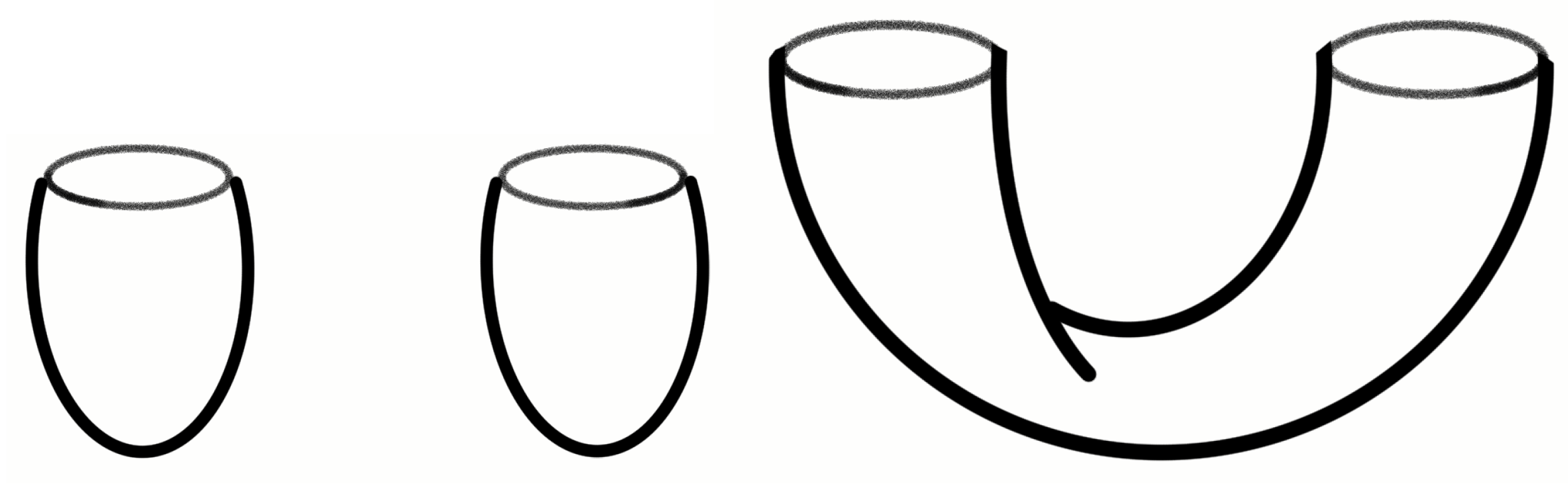
As we know, any type of quantum computer needs quantum entanglement to work [1,2]. In other words, it is a quantum algorithm, which is a unitary matrix always containing an entangling matrix controlled-NOT (C-NOT) for example. We discuss the possibility of modeling quantum entanglement with topological theories [3]; for example, knot theory, because in knot theory, the entanglement is transparent: the knot is entangled. The problem of the equivalence of quantum and topological entanglement is quite old, but still not closed [4,5,6]. Let us show several of the easiest examples of quantum entanglement in topological theory. We start with empty topological spaces with two spherical boundaries.

The notion of the separability of the state is quite clear in this case: the left state is clearly separable, while the right state is not. One can check the entanglement of the two states by computing their von Neumann entropy, for example via the replica trick. Here, each boundary corresponds to a subsystem.
The above states are pictorial representations of the wave function, which can explicitly be written as a functional integral. Hence, those states are pure. The corresponding density matrices are obtained by direct products of the wave function and its conjugate, that is a disjoint union of the manifolds of two copies of manifolds with an opposite orientation of the boundaries. The pictorial representations of the (unnormalized) density matrices:
![Universe 05 00060 i001]()

We denote the left density matrix as and the right one as . The normalized versions are:
![Universe 05 00060 i002]()

The normalized matrices satisfy the condition , where the trace is understood as gluing together the oppositely-oriented parts of the pictorial density matrices. In general, the result of such an operation would be a closed manifold, consequently a topological invariant. For example, the closed-manifold diagrams can be understood as:
![Universe 05 00060 i003]()

Here, Z is a functor between a category of topological spaces and a category of vector spaces. Since we associate vector spaces with boundaries, for the topological space without a boundary, Z gives the dimension of the associated Hilbert space, which, in the empty case, equals one. However, to keep the discussion more general, the diagrams above may stand for partition functions of closed three-manifolds with Wilson loops (links). It is now easy to compute the von Neumann entropy:
We use the replica trick [7] as follows:
We first compute the reduced density matrices. A partial trace in this case means gluing one of the “outgoing” two-boundaries with the corresponding “ingoing:” ones. For example,
![Universe 05 00060 i004]()
![Universe 05 00060 i005]() Consequently, one computes:
Consequently, one computes:
![Universe 05 00060 i006]() and the entanglement entropy reads:
and the entanglement entropy reads:
![Universe 05 00060 i007]() In the first case, the entanglement entropy vanishes identically, while in the second case, the result depends on the details of the Hilbert space (Wilson line insertions). In the simplest case, the invariant in is , so the second entropy also vanishes. Below, we will investigate the cases in which the entropy is non-trivial.
In the first case, the entanglement entropy vanishes identically, while in the second case, the result depends on the details of the Hilbert space (Wilson line insertions). In the simplest case, the invariant in is , so the second entropy also vanishes. Below, we will investigate the cases in which the entropy is non-trivial.


In particular, for a collection of Wilson lines closing around the non-contractible cycle of , the answer will be:
For the purposes of quantum coding, let us show a pictorial representation for an entangling operator:
![Universe 05 00060 i008]() It takes the separable state:
It takes the separable state:
![Universe 05 00060 i009]()


More complicated is the category of cobordisms of spheres with punctures; first of all, one can be restricted to the Temperley–Lieb subcategory. This forbids the chaining of strings (Wilson lines). Let us show that in this still somewhat trivial case, an entanglement operator looks as follows:
![Universe 05 00060 i010]()

It takes the unentangled state:
![Universe 05 00060 i011]()
![Universe 05 00060 i012]()


Another example that one can examine in terms of this schematic is the teleportation algorithm.
The idea of using the Temperley–Lieb (TL) algebra as a presentation of quantum algorithms is not very new. As an example, the work in [8] considered the equivalence of the quantum teleportation algorithm and the element of the TL algebra.
In the simplest realization of the quantum teleportation, A and B share an entangled pair, for example:
If A possesses a state that needs to be passed to B, then a measurement is performed on the first two bits of the product . If we understand measurement as a projection on some state , defined by the matrix elements in the measurement basis, then the state in possession of B after the measurement is ; provided the classical information on after the measurement B can recover the original state applying the unitary transformation M on the available qubit.
![Universe 05 00060 i013]() Teleportation looks somewhat trivial in the case of topological theories, since after all, those theories are independent of the space (and time) distance.
Teleportation looks somewhat trivial in the case of topological theories, since after all, those theories are independent of the space (and time) distance.

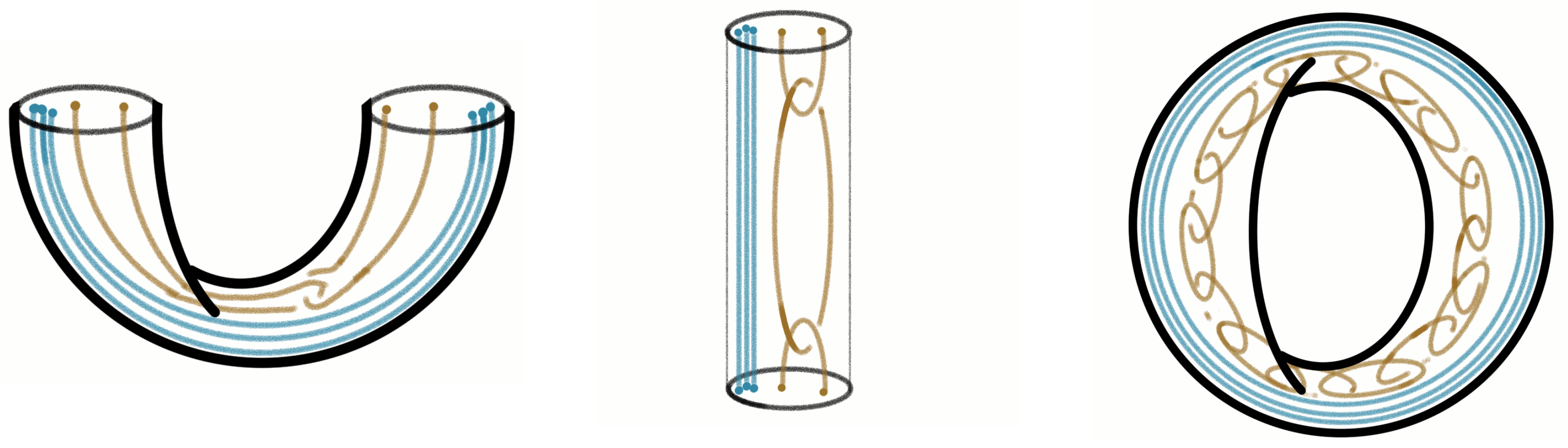
The most complicated generalization here is the possibility of chained (knotted) Wilson lines. In this case, we obtain knots and links in three-dimensional manifolds, see Figure 1.
Considering only leads to the whole theory of knot invariants. The most common and promising way [10,11] is to consider punctures on (the boundary), which correspond to points of a two-dimensional conformal block. The closed strings in in this construction correspond to the Wilson loops in a three-dimensional Chern–Simons theory. This idea provides one with strong machinery for computations of knot invariants. Namely, arbitrary representations of a general SU(N) group provide one with the colored HOMFLY polynomials.
2. Knots and Quantum Computers
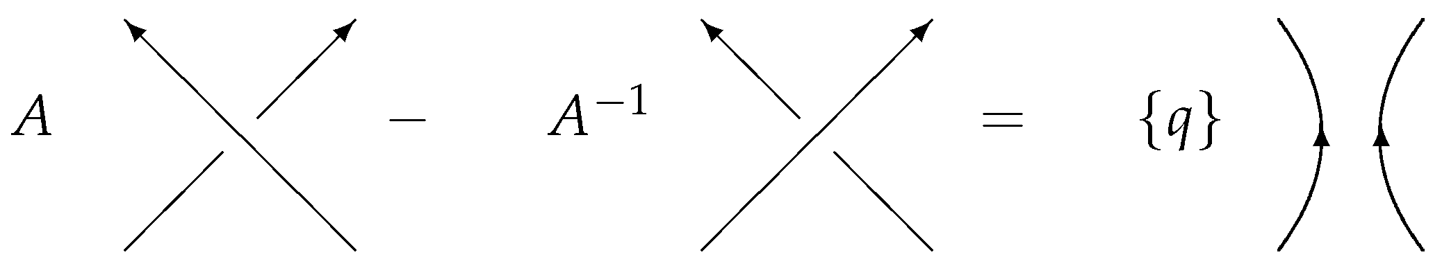
Let us briefly remind about the construction of the HOMFLY-PT (or just HOMFLY) polynomials. We focus on the HOMFLY-PT because it generalizes all the previously-known knot polynomials. It depends on two formal parameters: q and A; within the group theory consideration, , . A non-trivial fact is that the HOMFLY is a polynomial both in q and A. One can obtain other knot polynomials as specializations of HOMFLY: the Alexander polynomial (), the Jones polynomial (, which corresponds to the group), the special polynomial (). Moreover, we are going to consider the “colored” HOMFLY polynomial, where colored means that it also depends on the representation R; another (discrete) parameter. Of course, all these polynomials depend on the knot . We will denote the HOMFLY-PT polynomial as . Historically, the first one was the fundamental HOMFLY (), and the most straightforward way to compute it is to use the skein relations:

Here, we use the following notations: the curly brackets stand for the following difference and the square brackets for the quantum number: . The skein relations allow one to express the polynomial of any knot as a polynomial of the unknot (unknotted circle). The HOMFLY polynomial of the unknot within this framework is a common factor. General colored HOMFLY polynomials are obtained as Wilson lines in Chern–Simons theory. It may be considered as their definition; thus, the skein relations are straightforward to derive. The action for a Chern-Simons theory with the gauge group can be written as follows:
here is a coupling constant (it is quantized when one requires the topological invariance), and is the valued one-form (connection) or, in physical notations, a gauge vector field (do not confuse with the HOMFLY parameter A). The first formal parameter of the HOMFLY polynomial q in this formalism is expressed through a coupling constant and the size of the gauge group N:
The HOMFLY polynomial is exactly the Wilson average over the counter , which is tied in the corresponding knot:
and is eventually proportional to a Laurent polynomial in q and A.
For example, HOMFLY for a trefoil reads:
Technically, to calculate (16), one computes the quantum trace over the Wilson line with the insertion of R-matrices in all the crossings (in a 2d-knot projection). The R-matrix always acts on the product of two representations, and it can be defined either as the universal R-matrix from the quantum group or as a solution for the Yang–Baxter equation:
where indices stand for the representation on which the R-matrix acts. This equation should be considered as an equation for operators acting on the product of three representations.
As a matter of fact, the R-matrix is diagonal on the irreducible representation:
Its eigenvalue is:
where from the point of view of a quantum group, the formal parameter q is a parameter of deformation.
The -matrix in the concept of quantum computations is the very operator that provides entanglement [12].
The HOMFLY polynomials can be treated as matrix elements of unitary operators (up to a normalization factor), and the topological computing actually deals with the evaluation of an absolute value of the HOMFLY polynomials.
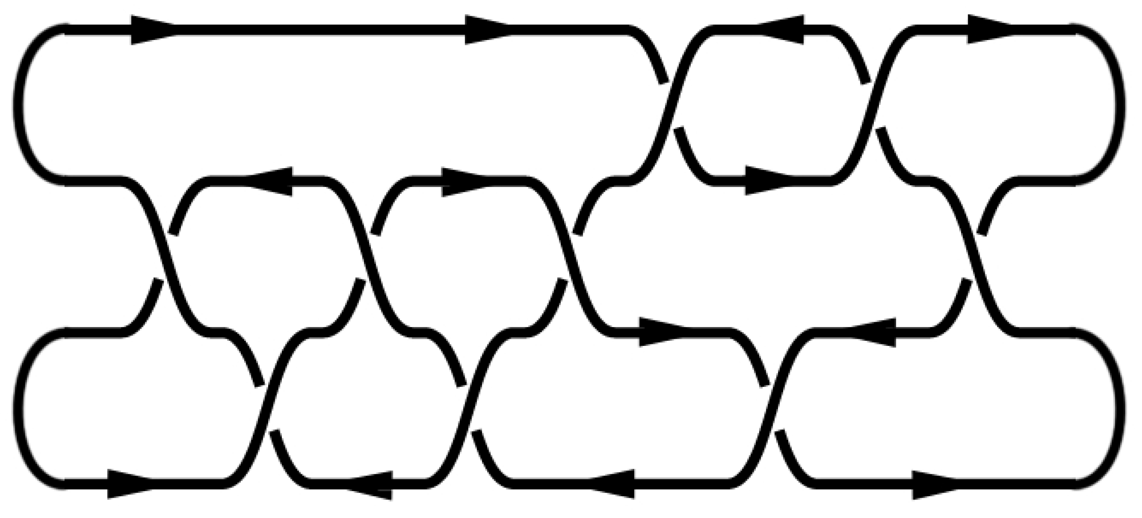
The plat (two-bridge) representation for the knot, see Figure 2, provides us with two R-matrices: associated with the crossing of the first and the second strands () and with the crossing of the second and the third strands ().
The last one in this representation is . We are going to discuss an example in the case of , i.e., . We consider only the non-trivial part of the matrices related to two irreducible representations , i.e.,
These two R-matrices can be considered as a set of universal gates on one q-bit. Note that here is obtained from by rotating the basis with a Racah matrix:
Note that both and are unitary at unimodular q. The reason is that the matrix elements of the Racah matrices are always constructed only from the quantum numbers, and these latter are real at unimodular q. These formulas are immediately generalized to the case so that the R-matrices do not change.
Moreover, one can realize the Hadamard (H) and (T) single q-bit operations by the matrices and by putting and , which corresponds to the group . In practice, one needs the combinations and , which are obviously:
since is related to exactly by the rotation with the Racah matrix . Thus, we finally come to the claim that the two R-matrices and , describing the two-bridge block in the plat representation, provide local gates in the space of single q-bit unitary matrices. In fact, one can choose almost arbitrary unimodular q and A preserving the matrices’ unitarity, while the values discussed above just demonstrate that one reproduces the standard universal set of gates.
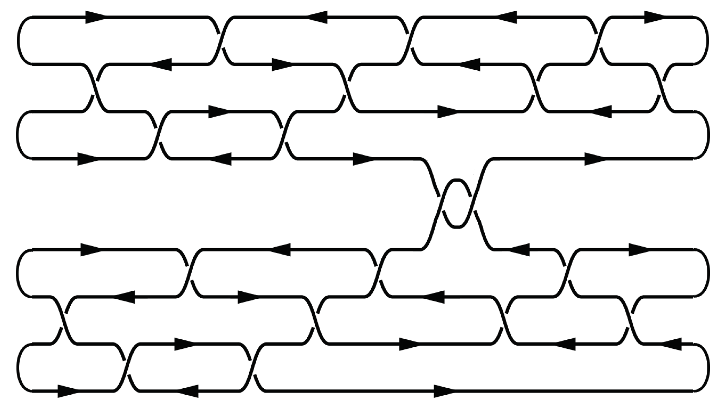
Note that one can generate a large enough set of unitary operations, considering matrices for large enough representations and acting on the product of a sufficient number of spaces. This is the way to generalize the knot/R-matrix construction to q-bits. Generalization to the many q-bit system requires an entangling matrix that acts on the tensor product of states. As a matter of fact, typical (i.e., at ) R-matrices and Racah matrices are entangling. Hence, the two-qubit case can be realized as the intertwined pair of two-bridge knots/links (see Figure 3): they are intertwined by the entangling matrices needed. This construction is not exactly the tensor product of two q-bits and is more complicated, but it is the best available so far.
The resulting quantum computer would be topological, hence, in theory, fault tolerant. However, practically, it is either truly topological by the construction (anyons), which has not been constructed yet, or there is a technical way to detect mistakes. In this example, since the HOMFLY polynomial has integer coefficients and any mistake, most likely, results in a non-integer coefficient, the mistake would be transparent. In an ideal system, the topology of a knot does not have a decoherence source. It could be introduced via the additional strands with “random” intersections.
Note that, within the knot/R-matrix approach, one starts from the R-matrices in the space of intertwining operators. This is because this construction is equivalent to dealing with the monodromies of conformal blocks of the WZNW (Wess-Zumino-Novikov-Witten) model [10], so that all the R-matrices act in the space of conformal blocks. Thus, in this part, the approach is very close to that described in the review [14], where the quantum computer is realized by moving points in the conformal blocks.
A totally different possibility one can consider is to act on the Wilson loop and/or manifold as a whole [15,16]. A distinct basis in such a Hilbert space can be introduced by the unknot (circle) along the non-contractible cycle in the bulk of a solid torus, colored with an integrable representation:
![Universe 05 00060 i014]() The scalar product of two basis vectors in the Hilbert space corresponds to gluing together two solid tori along the common boundary (with opposite orientation). Consequently, the result of this operation is a link invariant on :
i.e., it is indeed the orthonormal basis. The vector spaces associated with tori come with a discrete set of operations, namely the mapping class group. In the case of the Chern–Simons, the S and T generators have a well-known unitary representation:
Matrices S and T are defined here in the basis of integrable representations, labeled by integer . The mapping class group realizes local transformations on the Hilbert space of a single qudit. The S transformation swaps the two fundamental cycles of . Diagrammatically, we can illustrate this as follows:
The scalar product of two basis vectors in the Hilbert space corresponds to gluing together two solid tori along the common boundary (with opposite orientation). Consequently, the result of this operation is a link invariant on :
i.e., it is indeed the orthonormal basis. The vector spaces associated with tori come with a discrete set of operations, namely the mapping class group. In the case of the Chern–Simons, the S and T generators have a well-known unitary representation:
Matrices S and T are defined here in the basis of integrable representations, labeled by integer . The mapping class group realizes local transformations on the Hilbert space of a single qudit. The S transformation swaps the two fundamental cycles of . Diagrammatically, we can illustrate this as follows:
![Universe 05 00060 i015]() In general, the scalar products of states in the Hilbert space are path integrals of the TQFT (topological quantum field theory) on different manifolds. Different ways of gluing tori produce a set of closed three manifolds known as Lens spaces (Seifert spaces). Using this picture of cobordisms of , one can compute the entanglement entropy directly associated with links and, thus, quantify the relation of the topological and quantum entanglements. In particular, the state, which corresponds to a Hopf link, appears to be maximally entangled, while unlinked circles have zero entanglement entropy.
In general, the scalar products of states in the Hilbert space are path integrals of the TQFT (topological quantum field theory) on different manifolds. Different ways of gluing tori produce a set of closed three manifolds known as Lens spaces (Seifert spaces). Using this picture of cobordisms of , one can compute the entanglement entropy directly associated with links and, thus, quantify the relation of the topological and quantum entanglements. In particular, the state, which corresponds to a Hopf link, appears to be maximally entangled, while unlinked circles have zero entanglement entropy.


3. Summary
The main idea of this review is to emphasize the relation between the quantum entanglement and the topological entanglement. While the topological entanglement is intuitive, it can serve as a model for the quantum entanglement. Another purpose is to show that there are two different ways to look at the topological code space and, hence, model a quantum computer with knot theory. The first one is the R-matrix formalism; the second one is the mapping class group formalism. These structures are absolutely different, but both have the desirable feature of a topological stability.
Funding
This research was funded by Russian Science Foundation Grant 18-71-10073.
Acknowledgments
The authors are indebted to D. Melnikov, A. Mironov, A. Morozov, and An. Morozov for fruitful collaboration.
Conflicts of Interest
The author declares no conflict of interest.
References
- Kitaev, A.Y. Fault-Tolerant Quantum Computation by Anyons. Ann. Phys. 2003, 303, 2–30. [Google Scholar] [CrossRef]
- Freedman, M.H.; Kitaev, A.; Wang, Z. Simulation of topological field theories by quantum computers. Commun. Math. Phys. 2002, 227, 587. [Google Scholar] [CrossRef]
- Melnikov, D.; Mironov, A.; Mironov, S.; Morozov, A.; Morozov, A. From Topological to Quantum Entanglement. arXiv, 2018; arXiv:1809.04574. [Google Scholar]
- Aravind, P.K. Borromean entanglement of the GHZ state. In Potentiality, Entanglement and Passion-at-a-Distance; Cohen, R.S., Horne, M., Stachel, J.J., Eds.; Springer: Kluwer, The Netherlands, 1997; pp. 53–59. [Google Scholar]
- Kauffman, L.H. Knot Logic and Topological Quantum Computing with Majorana Fermions. arXiv, 2013; arXiv:1301.6214. [Google Scholar]
- Kauffman, L.H.; Mehrotra, E. Topological Aspects of Quantum Entanglement. arXiv, 2018; arXiv:1611.08047. [Google Scholar]
- Dong, S.; Fradkin, E.; Leigh, R.G.; Nowling, S. Topological Entanglement Entropy in Chern-Simons Theories and Quantum Hall Fluids. J. High Energy Phys. 2008, 2008, 16. [Google Scholar] [CrossRef]
- Kauffman, L. Teleportation topology. Opt. Spectrosc. 2005, 99, 227. [Google Scholar] [CrossRef]
- Mironov, A.; Morozov, A.; Morozov, A. Tangle blocks in the theory of link invariants. J. High Energy Phys. 2018, 2018, 128. [Google Scholar] [CrossRef]
- Witten, E. Quantum Field Theory and the Jones Polynomial. Commun. Math. Phys. 1989, 121, 351–399. [Google Scholar] [CrossRef]
- Atiyah, M.F. The Geometry and Physics of Knots; Cambridge University Press: Cambridge, UK, 1990. [Google Scholar]
- Melnikov, D.; Mironov, A.; Mironov, S.; Morozov, A.; Morozov, A. Towards topological quantum computer. Nucl. Phys. B 2018, 926, 491. [Google Scholar] [CrossRef]
- Bar-Natan, D. The Knot Atlas. Available online: http://www.katlas.org (accessed on 13 February 2019).
- Nayak, C.; Simon, S.H.; Stern, A.; Freedman, M.; Sarma, S.D. Non-Abelian anyons and topological quantum computation. Rev. Mod. Phys. 2008, 80, 1083. [Google Scholar] [CrossRef]
- Balasubramanian, V.; Fliss, J.R.; Leigh, R.G.; Parrikar, O. Multi-Boundary Entanglement in Chern-Simons Theory and Link Invariants. J. High Energy Phys. 2017, 2017, 61. [Google Scholar] [CrossRef]
- Balasubramanian, V.; DeCross, M.; Fliss, J.; Kar, A.; Leigh, R.G.; Parrikar, O. Entanglement Entropy and the Colored Jones Polynomial. J. High Energy Phys. 2018, 2018, 38. [Google Scholar] [CrossRef]
Figure 1.
A state with two “chained” Wilson lines for an arbitrary number of punctures (left). The reduced density matrix of the corresponding state (center). of a chain link that computes (right). See [9] for a particular example.
Figure 1.
A state with two “chained” Wilson lines for an arbitrary number of punctures (left). The reduced density matrix of the corresponding state (center). of a chain link that computes (right). See [9] for a particular example.

Figure 2.
Plat representation of the knot [13].
Figure 2.
Plat representation of the knot [13].

Figure 3.
The plat representation corresponding to two-qubits: four-bridge case.

© 2019 by the author. Licensee MDPI, Basel, Switzerland. This article is an open access article distributed under the terms and conditions of the Creative Commons Attribution (CC BY) license (http://creativecommons.org/licenses/by/4.0/).
Share and Cite
MDPI and ACS Style
Mironov, S. Topological Entanglement and Knots. Universe 2019, 5, 60. https://0-doi-org.brum.beds.ac.uk/10.3390/universe5020060
AMA Style
Mironov S. Topological Entanglement and Knots. Universe. 2019; 5(2):60. https://0-doi-org.brum.beds.ac.uk/10.3390/universe5020060
Chicago/Turabian StyleMironov, Sergey. 2019. "Topological Entanglement and Knots" Universe 5, no. 2: 60. https://0-doi-org.brum.beds.ac.uk/10.3390/universe5020060
Note that from the first issue of 2016, this journal uses article numbers instead of page numbers. See further details here.