Qualitative Analysis of the Dynamics of a Two-Component Chiral Cosmological Model


1
Inter-University Department of Space Research, Samara National Research University, 443086 Samara, Russia
2
Department of Theoretical Physics, Ulyanovsk State University, 432970 Ulyanovsk, Russia
3
Department of Physics and Technical Discipline, Ulyanovsk State Pedagogical University, 432071 Ulyanovsk, Russia
4
Department of Physics, Bauman Moscow State Technical University, 105005 Moscow, Russia
5
Institute of Physics, Kazan Federal University, 420008 Kazan, Russia
*
Author to whom correspondence should be addressed.
†
These authors contributed equally to this work.
Universe 2020, 6(11), 195; https://0-doi-org.brum.beds.ac.uk/10.3390/universe6110195
Submission received: 14 September 2020
/
Revised: 9 October 2020
/
Accepted: 15 October 2020
/
Published: 24 October 2020
(This article belongs to the Special Issue Selected Papers from the 17th Russian Gravitational Conference —International Conference on Gravitation, Cosmology and Astrophysics (RUSGRAV-17))
Abstract
:We present a qualitative analysis of chiral cosmological model (CCM) dynamics with two scalar fields in the spatially flat Friedman–Robertson–Walker Universe. The asymptotic behavior of chiral models is investigated based on the characteristics of the critical points of the selfinteraction potential and zeros of the metric components of the chiral space. The classification of critical points of CCMs is proposed. The role of zeros of the metric components of the chiral space in the asymptotic dynamics is analysed. It is shown that such zeros lead to new critical points of the corresponding dynamical systems. Examples of models with different types of zeros of metric components are represented.

1. Introduction
A Chiral Cosmological Model (CCM) is a self-gravitating nonlinear sigma model (NSM) containing the interaction potential and employed in cosmological spacetimes. A detailed description of a historical development and terminology of the CCM, and its application in cosmology can be found in the review [1]. We just mention here that the term “chiral” is considered in the sense of short equivalent to the general chiral NSM with a Riemannian metric as a target space in accordance with terminology in the review [2]. Paradoxically, this term has been applied to pure bosonic NSM which has no relation to chiral symmetry because pure bosonic NSM does not contain the spinor fields. Thus the term "chiral" means that the scalar fields are not free and take values on some nonlinear manifold. Further progress of CCM and connection to multifield models reflected in the article [3]. N-field CCM analyzed in the work [4].
The search for exact solutions in the CCM is based as a rule on the study of a model with known character of evolution, i.e., when a scale factor or the Hubble parameter is given [5,6]. Such approach means that we are working within the framework of a chiral space deformation method [1], i.e., we define the geometric parameters (the components of the chiral metric) and the potential both corresponding to this evolution.
Chiral cosmological models as well as multifield models are a natural generalization of the models with one scalar field. The single scalar field models were actively exploit in inflationary cosmology (for a survey of exact solutions construction, see, for example, [7,8] and the monograph [9]). The peculiarity of CCMs is that they take into account the potential and kinetic interactions between fields. Until recently, as far as we know, these characteristics were reconstructed from observational data only in the work [10].
It is well-known that models with a single scalar field non-minimally coupled to gravity as well as gravity models can be always transformed to models with minimally coupled scalar field with the canonical kinetic term by the metric and scalar field transformations [11]. In contrast to this, models with a few fields non-minimally coupled with gravity, in general, do not admit such a transformation [12]. After the metric transformation, one obtains the CCMs in the Einstein frame [13,14]. The multifield inflationary models do not contradict the Planck data [15,16] and are being actively studied [13,14,17,18]. It was recently argued that compared to single field models, a system with several scalar fields, including CCM, can better reconcile with observation. For instance, it was shown in Ref. [13] that additional degrees of freedom can produce enough power in the isocurvature perturbations which could account for the anomaly in the Planck observation data.
It is worth to mention about application of CCMs for description of Dark Matter (DM) and Dark Energy (DE) [1,10]. In [19] it was given analysis of DE contribution to critical density, the ratio of the kinetic and potential energies, deceleration parameter, effective equation of state (EoS) on the basis. A comparison of (proposed in the article [20]) CDM with the CDM model was performed also.
In addition to the a priori specified symmetry and reconstruction of the chiral metric and potential from observational data we can mention about another constraint on the CCM characteristic. Such constraint can arose when the transition from the gravity theory with higher derivatives in the Jordan frame is made to the Einstein frame with several scalar fields [21]. The last model can be presented in the form of the CCM [22]. Indeed, for example, the kinetic scalar curvature extended f(R) gravity was investigated by “direct” method (direct analysis of equations of the 6th order with respect to a scale factor and searching of their solution) in the works [23,24]. On the other hand Naruko et al. [21] shows the possibility to make transition from gravity to Einstein gravity with several scalar fields, using the Lagrangian multiplier method and the Weyl conformal transformation. In the work [25], the dynamic equations of the gravitational and scalar fields were derived by direct variation of the gravitational field metric and by variation of the scalar fields. Equations of cosmological dynamics in the Friedman–Robertson–Walker (FRW) metric in the presence of an perfect fluid are also derived. In the work [22], similar equations for gravity were investigated on the basis of a transition to the CCM with additional inclusion of matter fields.
The good correspondence with observation data for CCM derived from modified gravity theory with a kinetic scalar curvature was shown in [26]. There also new method of cosmological parameters calculation based on reduction of two-fields model to standard one with a single scalar field is proposed. Parametric correspondence to observational data is shown for massive scalar field, power-law and intermediate inflation.
The study of cosmological models by the methods of qualitative analysis of dynamical systems has been used for a long time, which is reflected in the monograph of Bogoyavlensky [27]. The active use of qualitative analysis of dynamical systems techniques in models of cosmological inflation began in fact with the pioneering work of Starobinsky [28,29] and the works of Belinsky with co-authors [30]. Many works with single scalar field devoted to searching of exact solutions [7,8,9] as well as in the context of qualitative analyses (see, for example, [31,32,33,34] and literature quoted therein) have been performed.
Investigation the cosmological models with qualitative analysis executed in a series of works [35,36,37,38] Qualitative and numerical analysis were performed for cosmological models with a phantom scalar field [35,36] with asymmetric scalar doublet (see, [37] and literature quoted therein) with canonical and phantom fields [39,40]. We note that kinetic interaction between scalar fields were not considered in all these works.
Another example is the approach outlined in [41], where the features of the evolution of cosmological models were considered from the point of view of their dynamics on the energy plane. An important aspect of these works is the ability to establish all the basic asymptotes of the models without having exact solutions. Accompanying this qualitative information with phase diagrams constructed by numerically solving the equations of cosmological models, it is possible to obtain a very visual way to analyze the processes of the evolution of the Universe within the framework of the assumptions made.
In this paper, a qualitative analysis similar to that carried out in the works [36,38,42] is applied to a qualitative study of the properties of cosmological models with field matter in the form of a two-component chiral cosmological model. The main task of this work will be to establish the asymptotic properties of the models under fairly general assumptions about the nature of the models themselves, including the potential of field interaction and the parameters of the internal geometry of the chiral space.
The dependence of the asymptotic properties of the models on the functional form of the interaction potential in the models with one scalar field has been well studied in the works listed above. However, the role of the components of the chiral metric has not been studied in [36,38,42]. Therefore, the main goal of this work is to elucidate those features of the chiral metric components that can significantly change the asymptotic dynamics of cosmological models.
The article is organised as follows. Section 2 gives introduction to CCM with N-fields. Section 3 contains the derivation of the standard form of a dynamical six-dimensional system of the 2-CCM. The main and special critical points we introduce and find in Section 4. In Section 5 we perform asymptotical analysis of the 2-CCM dynamic. We find and give classification for the main critical points. The special critical points are investigated for the case of flat chiral space as well. In Section 7 we investigate the 2-CCM with flat chiral space by numerical methods and analyse the graphs of model’s parameters. Section 8 is devoted to investigation of influence of the special critical points on possible breaking the symmetry of the potential with respect to the "rolling" of the model fields into symmetric critical points. In Section 9 we make conclusion of the investigation results.
2. Chiral Cosmological Model
The action of CCM as the action of the self-gravitating nonlinear sigma model (NSM) with the potential of (self)interactions [43,44] reads:
where R being a scalar curvature of a Riemannian manifold with the metric , —Einstein gravitational constant, being a multiplett of the chiral fields (we use a notation ), being the metric of the target space (the chiral space) with the line element
The energy-momentum tensor for the model (1) reads
The Einstein equation can be presented in the form
which simplify the derivation of gravitational dynamics equations.
3. Derivation of a Dynamical System of the 2-CCM
The two-component CCM with a diagonal metric of the chiral space [45] is represented by the action:
Here we set Moreover, (gaussian coordinates) and are the metric components of the target (chiral or internal) space with the linear element
In the Friedmann–Robertson–Walker (FRW) spatially flat metric
the dynamic equations of the 2-CCM have the following form [1]:
In this system the first two Equations (9) and (10) are the chiral fields equations and the last two Equations (11) and (12) are Einstein-Friedmann ones.
To analyse these equations we must write it in the dimensionless form. To this end let us introduce dimensionless variables as follow
The argument t and functions in numerators of the system (9)–(12) are dimensional functions. To make this system dimensionless one we must impose the following relations on the scale values:
Moreover, we choose in further numerical investigations. Therefore the dimensional gravitational constant is connected with the fields scale by the relation .
Using Equations (9) and (10) we can obtain an important expression for the interaction potential as a function of a scale factor and, consequently, as a function of time . To this end let us introduce auxiliary variables
which allow to write the system of equations in the form of the dynamical system.
Multiplying Equation (16) by and Equation (17) by , then adding up the results, we obtain at the following equation:
Equation (11) can be written in new variables as follows:
From here we find:
Substituting this Equation into (18), we finally receive the following relation:
where .
This equation is a standard element of cosmological models with scalar fields [9]. It is not difficult to check that substituting (20) into (21) we get an identity.
Taking into account that one of the field equations is a consequence of the other three equations, we can exclude Equation (12) from the system (9)–(12). After that we can reduce the system (9)–(11) to the standard form of a dynamical system. To this end we choose the following as dynamic variables of the system: . The system of Equations (9)–(11) can now be reduced to the following form:
This system is a 6-dimensional (6D) dynamic system for which the Equation (19) is the integral of motion. This integral gives 5D hypersurface in 6D embedding space. Phase trajectories belong to this 5D hypersurface.
The system of Equation (22) is adopted for numerical calculations. Some of the equations contain chiral metric component in the denominators. Formally, when one set in CCM dynamic Equations (9)–(12) we get the single field model. However, in numerical analysis, due to the singularity at points , when the trajectories approach them, the calculation is cut off because of the limited accuracy of the calculation. Therefore in our analysis we can set .
4. Critical Points of the 2-CCM
The constructed dynamical system (22)–(25) of FRW cosmology equations allows us to carry out the general analysis of the evolution of the two-component CCM, as well as a qualitative analysis of its asymptotic behavior.
Let us pay attention to Equation (22). This equation is derived from the combination of Einstein-Friedmann Equations (11) and (12). We suggest that the metric components of the target space and are non-negative functions of and :
Then from Equation (12) one can see that for all t:
Moreover, our suggestion (26) in the present work means that the phantom fields are not considered.
4.1. Critical Points for
Let us study the case when the chiral metric component does not vanish anywhere: . Equating the derivatives in (22)–(25) to zero one can derive the equations corresponding to stationary points
From here we find:
where are the values of the fields at the extremes of the interaction potential. The extremes are defined from Equations (28) and (29). We will call such critical points the main ones.
Thus, for all the main critical points, the value of the Hubble parameter is determined by the value of the interaction potential at the corresponding extremum.
4.2. Critical Points for
If the function vanishes under some values of and then additional critical points, connected with zeros of , can appeared. Such critical points we will call the special critical points.
Let us denote as and the values of the fields for which:
We represent in the vicinity of the point the Equations (23) and (24) of the system (22)–(25) in the following form:
It is not difficult to see that in this case at the point , where vanishes, the last equations take the following form:
These equations no longer contain derivatives of the potential and automatically vanish under the condition , which is the consequence of the rest equations of the system. Thus, in the general case, the new special critical point will not coincide with any of the main critical points, which are associated by definition with the minima of the interaction potential. For these singular points, its defining equations are:
In this case, the limiting value of is determined by the value of the potential at the special critical point, but does not at the extremum of the potential.
Special critical points can form continuous curves in the function space. The variety of possible situations in this case requires a separate analysis, which is beyond of the scope of this article.
However, we will pay attention here to one simple situation which can play an important role in cosmological dynamics. For this, let us choose in the form corresponding to the surface of rotation:
Let us assume that for the field value : . Then, in the vicinity of in the target space, the Equations (23) and (24) of the system (22)–(25) take the following form:
Equation (36) of this system does not contain the factor , which vanishes at the point . Therefore, the equations for the special critical point will be as follows:
Note that request is absent here and the potential has not to be an extremum.
5. Asymptotical Analysis of the 2-CCM Dynamic
The presence of two types of critical points of the model, main and special, leads to more complex analysis of the dynamics in their vicinity using the first order perturbation theory. In this section, based on perturbation theory, complete classification of the main critical points of 2-CCM is carried out. The perturbation theory near special singular points turns out to be much more diverse than the main ones, which requires separate work. Therefore, in this section, perturbation theory is applied only for one type of special points associated with the point zeros of the metric components of the chiral space.
5.1. Main Critical Points
To obtain the equations for perturbations in the first order we introduce the following new (small) variables:
It is assumed here that .
Substituting these relations into the original system (22)–(25) and discarding the terms of the second order of smallness, we find:
Here:
We see from the relations above that the asymptotic parameters of the fields in the first order of the perturbation theory do not depend on the choice of the target space components and , if does not have singularities.
The equation for is integrated independently of the other equations. The solution is
Equations for variables and take the following form:
Note that this system in a certain sense is an analogue of the mechanical system of motion of the ball in a potential field of forces. Its difference from such system is the presence of the specific resistance force proportional to the ball speed with a damping decrement . Looking for particular solutions of this system in the following form:
we obtain the following algebraic system of equations:
As a result, the characteristic equation for can be written as follows:
where we introduce the notation:
From the Equation (40) we find:
From here we obtain the characteristic numbers:
where and . Hence it follows that, depending on the kind of the quadratic form of the interaction potential near the extreme, there are several different options of solutions behavior. These options are determined by the magnitude of the eigenvalues which are defined by the relationship between and the value of .
We can divide all possible situations into two general classes. The first class includes all critical points for which the value of the interaction potential is strictly positive: . For this case, the asymptotic value of is nonzero, which means that the universe goes asymptotically to the stage of exponential expansion (inflation).
The second class corresponds to zero value of the interaction potential at the critical points and zero asymptotic value of the Hubble parameter: . This option means , i.e. the scale factor a asymptotically goes to some constant value (stationary universe).
5.2. Class of the Main Critical Points
Let us study class of the main critical points. We have the following subdivision of the main critical points for this class.
A1.
This condition means:
From here we get:
All eigenvalues have negative real part. Therefore these fixed points are stable focuses on the phase plane. Since the imaginary part of the eigenvalues does not simultaneously vanish, these points cannot be nodes.
A2.
Under this condition, we have:
The eigenvalues of the equations for perturbations will be as follows:
The first two roots are real, but among them there can be both negative and positive ones, what means, in the general case, the instability in neighborhood of these points. For stability in these points, it is enough to impose the additional condition:
With this condition the points will be the focus. Besides, the singular point can coincide with the saddle point of the potential. Such coincidence distinguishes the dynamic system from the mechanical model of rolling the ball into the minimum of the potential hole.
A3.
When this condition is true we have
From here we obtain:
This option splits into two additional ones.
A3a. ,
The eigenvalues in this variant are:
All eigenvalues are real. For stability, all four numbers must be negative. However, it is not possible due to the condition . This means that all such points are unstable.
A3b. ,
The eigenvalues in this case are:
The stability condition is reduced to additional one:
Then the point is the focus.
The general conclusion for the class is like follow. All variants of the non-degenerate quadratic form of the potential near the critical stable point lead to conclusion that this point is the focus. An exception is the case for which the critical point is a node, not a focus. This requires that:
The latter means that the point is the minimum of the potential, the potential itself near the critical point has a symmetric quadratic form (), and its value is determined by the second derivative U at this point.
5.3. Class of the Main Critical Points
In the class of the main critical points the eigenvalues are:
Here and .
The class almost completely reproduces the subdivisions of the class . The difference is the option.
B1.
Under this condition we have:
This means that all eigenvalues are purely imaginary, the critical point coincides with the minimum of the potential and it is the center. In class , this option corresponds to focus.
B2.
In this case, the critical point coincides with the saddle point of the potential and it is not stable under all other conditions. In the class , the saddle point of a potential can be a focus.
B3.
Since we have
The critical point coincides either with the saddle point or with the maximum of the potential. The eigenvalues are as follows:
It is clear that at least one of these numbers turns out to be real with positive real part. This means that such critical points are unstable.
The considered variants of the asymptotic behavior of the system describe only the main possibilities. There are several specific options for the system behavior in some special situations. The first such situation is the case when the interaction potential is everywhere equal to zero . In this circumstance, we have:
In addition, in the limit , the Hubble parameter tends to zero, which leads to power-law inflation or the Friedman expansion regime, which requires separate analysis.
Another important feature of this system is the possibility of occurrence of critical points associated with such field values, at which the metric component vanishes. Analyzing the behavior of the system near this point turns out to be difficult. However, it will be shown below that at such point an additional attracting point can appear on the phase plane.
5.4. Special Critical Points
The analysis of the behavior of the system (22) near special critical points even in the first order of perturbation theory is a difficult problem. To investigate it one needs analyzing equations in orders of perturbation theory greater than the first. Therefore, in this work, we are not consider all possible variants of special critical points. Instead, we analyze only few important choices of the function in the form (34). Let us start with the choice:
This choice corresponds to flat internal chiral space, in which the field plays the role of the radial coordinate, and - the angular one for the polar coordinate system. The metric of the chiral space with our choice is
To study special critical points, we assume that the minimum of the potential is shifted from the point . Otherwise, the analysis of the problem also becomes more complicated and it will not show the special behavior of the system which we want to illustrate further by numerical calculation. Since depends only on , the system of equations for perturbations will take the following form:
The introduced definitions here are:
All derivatives are calculated at special critical point with coordinates , where the Equation (37) are fulfilled. In the case under consideration, , and is determined from the condition:
The Equation (42) retains the terms of the largest second order. This equation does not contain first-order terms.
If we choose we have: . At this point:
Therefore, the Equation (42) vanishes identically. In such circumstance it is necessary to consider this equation in the third order. In this case this equation is reduced to the condition:
Only one solution is not trivial: . In this case, near the special critical point, with respect to the first-order perturbations of the field , it takes the following form:
Therefore, when approaching special critical point, only the field will oscillate.
6. The 2-CCM with Massive Chiral Fields and
Let us study 2-CCM with a potential corresponding to the massive scalar field theory. Such potential is actively used in inflationary cosmology [9]. As standard type of massive two-fields potential we consider the potential of the following form:
Here P and Q are the real numbers determining the position of the minimum of the potential on the plane. The number determines the value of the potential at the minimum, and the parameters and characterize the values of the masses of scalar fields.
At this stage we choose the chiral metric components in the following form:
We easily find that this model has a unique fixed point , which is steady focus. According to the earlier analysis, the function does not vanish anywhere (possibly only at infinity), therefore there are no special critical points in this version of the model.
An example of the behavior of such a model is shown in Figure 1, Figure 2 and Figure 3. The model matches the choice of metric component and a potential:
Figure 1, Figure 2 and Figure 3 show the graphs of the behavior of the model parameters near the critical point for the values of the parameters .
7. The 2-CCM with
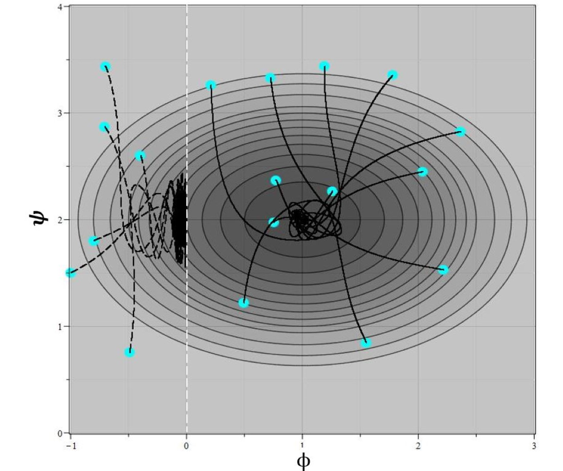
As the example of 2-CCM, in which, in addition to the main critical point, there is also one special point. Let us consider a model with a potential (46) where the minimum is shifted to the point :
In this case, we choose the functional form of the metric component in the following form:
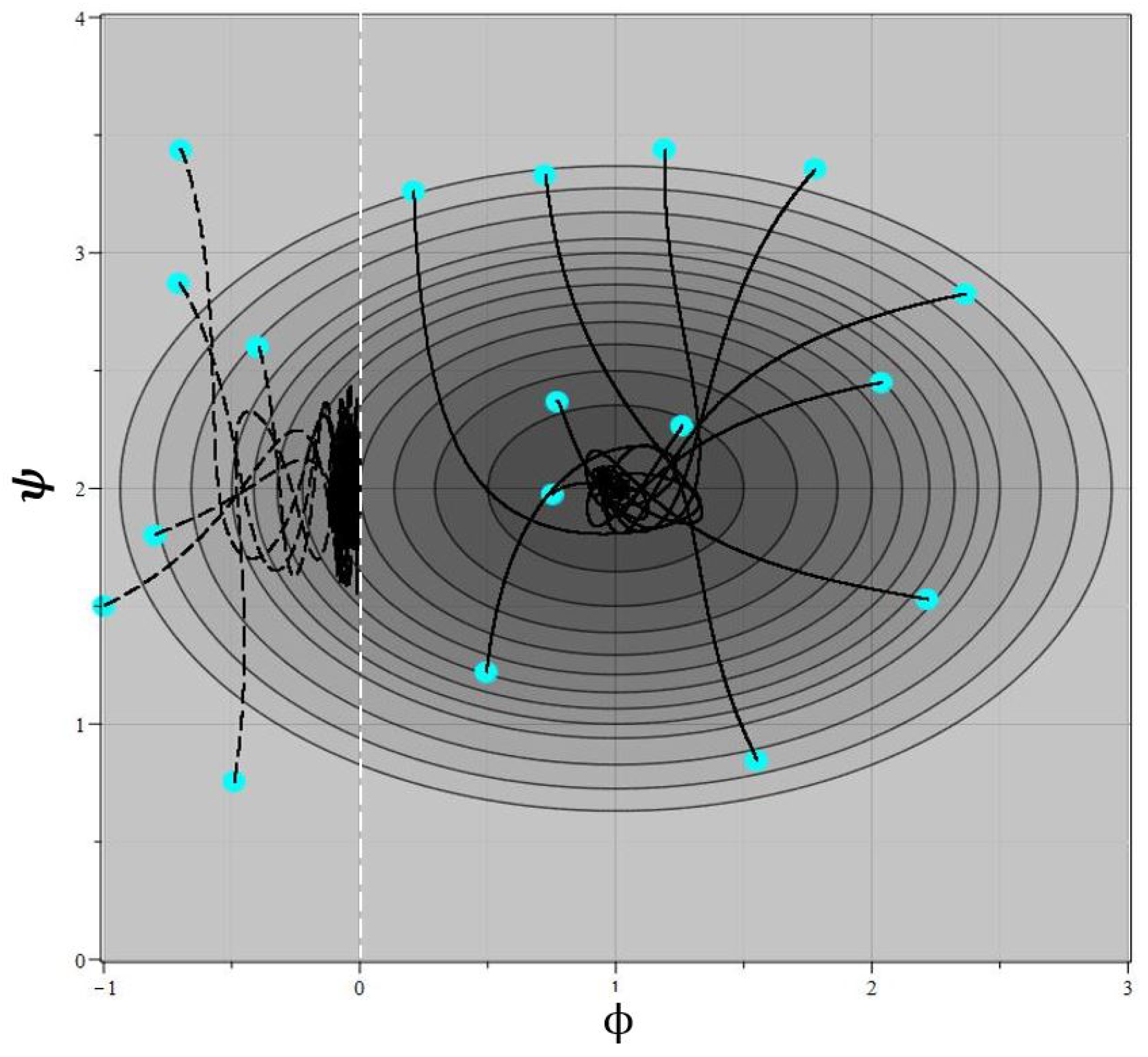
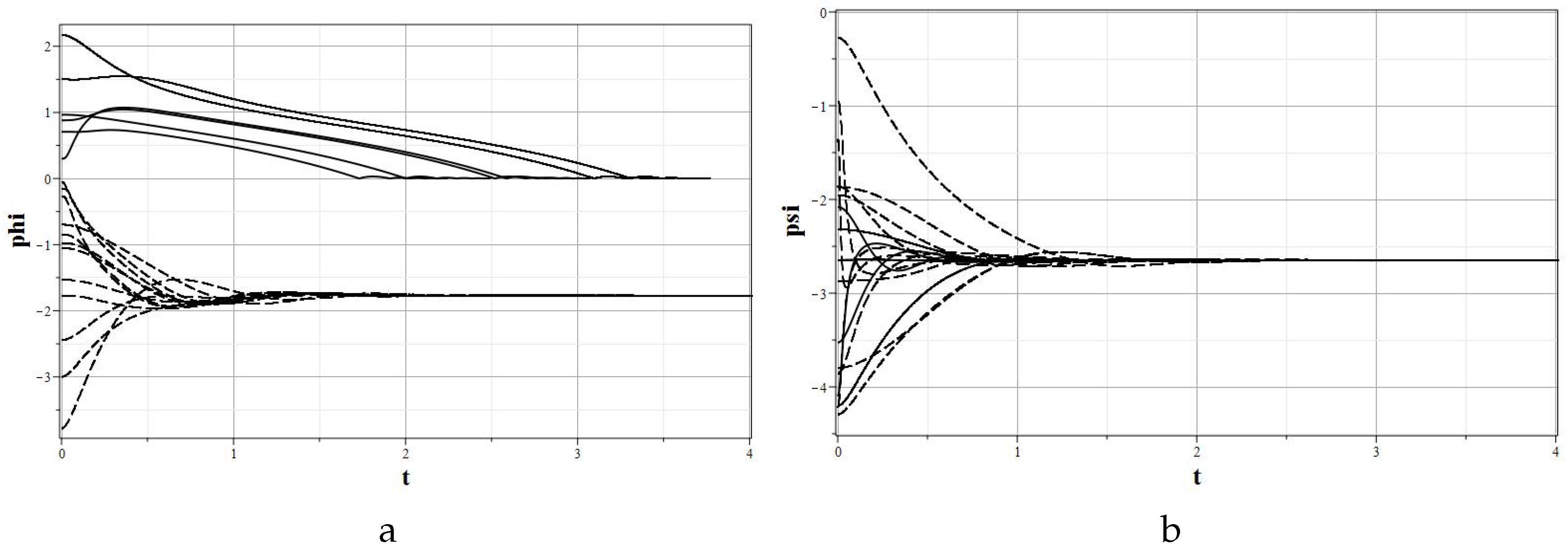
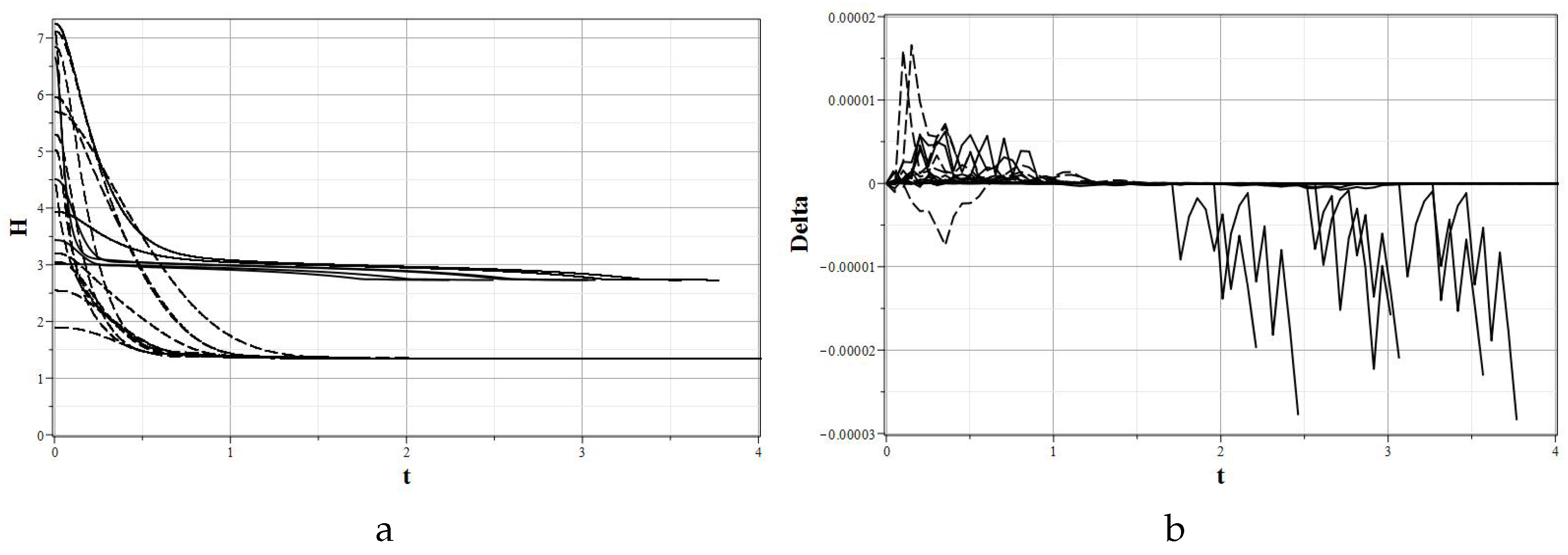
In this case, a special critical point appears at the point with coordinates . The behavior of the model parameters for various initial conditions is shown in Figure 4, Figure 5 and Figure 6.
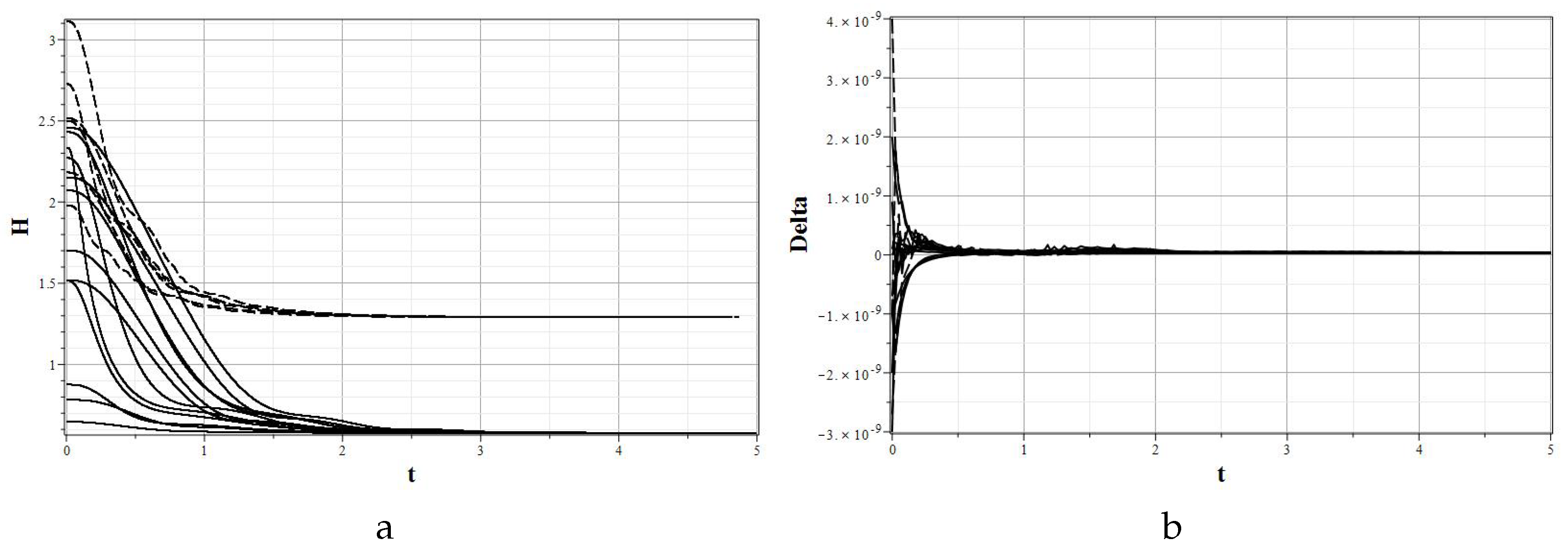
In Figure 6 the graphs of the dependence of the Hubble parameter on time and values of the integral of motion are shown.
It is not difficult to see that the phase curves in the plane, depending on the position of the initial point, tend to both singular points as . If at the initial point , the phase trajectories converge to a special critical point, and in the case —to the main one. The specificity of a special critical point is that its type cannot be characterized using standard definitions: node, center, focus, saddle. As was shown, when approaching the considered special singular point, only one field oscillates in the first order, which distinguishes the situation from both an attracting node and an attracting focus. Moreover, this point is attracting only in the half-plane , and in the half-plane this point looks like a saddle. Therefore, this point is difficult to describe even in terms of “half focus”, “half center” or “half saddle”. For this behavior of the model on the plane , we can offer simple mechanical analog, which was mentioned in the analysis of the main singular points. The observed dynamics is analogous to the rolling of a ball into a hole under the action of gravity in the presence of friction forces. In the absence of zeros for the function for finite values of and , rolling at all initial positions of the ball leads to the main minimum. The presence of zeros in the function is similar to the appearance of insurmountable barriers to the motion of the ball. As a result, by analogy with a ball, the fields “roll” to the conditional minimum of potential energy located on the barrier, which is shown in Figure 4 by a vertical dotted line. This analogy illustrates the tendency of all trajectories in the model with at to the conditional minimum of the potential at the point . This behavior, most likely, is reproduced with more complex structures of the zeros of the function . However, this requires a separate analysis beyond the scope of this article.
Note also that the analysis of the phase curves in the plane (see Figure 4) demonstrates oscillations of the field near a special critical point in the absence of field oscillations, which is in complete agreement with the formula (44) obtained earlier for a special critical point of the type considered here.
As the plots of the dependence and demonstrate, the asymptotic behavior of the Hubble parameter essentially depends on the critical point to which the system moves, depending on the initial condition. The graphs in Figure 6a show that the asymptotic values of the Hubble parameter calculated in advance completely coincide with their numerical value. The graph in Figure 6b shows that the constructed solutions were found with high accuracy, since the calculations were carried out using the dverk 78 procedure of the Maple mathematical package using the Runge–Kutta method of 7–8 orders.
Let us consider another example showing similar behavior of the model but with more complicated potential of the following form:
This potential has one minimum in the point . As in the previous case, . The corresponding graphs of the model parameters change over time are shown in Figure 8.
As in Figure 4, in Figure 7 the vertical dashed line depicts a “barrier” on which a special critical point lies. In accordance with the equations of the system (44), only the field oscillates near the special critical point. This is clearly seen from the graphs in Figure 8, which illustrate the evolution of fields near a special critical point. On the Figure 7, the oscillations of the field are small and therefore hardly noticeable. In Figure 9 it shown the graphs of the dependence of the Hubble parameter on time and values of the integral of motion. The calculations for the model with the (49) potential were carried out using the ck45 procedure of the Maple mathematical package using the Runge–Kutta method of 4–5 orders (using the dverk78 procedure for this model leads to an earlier termination of calculations near singular points).
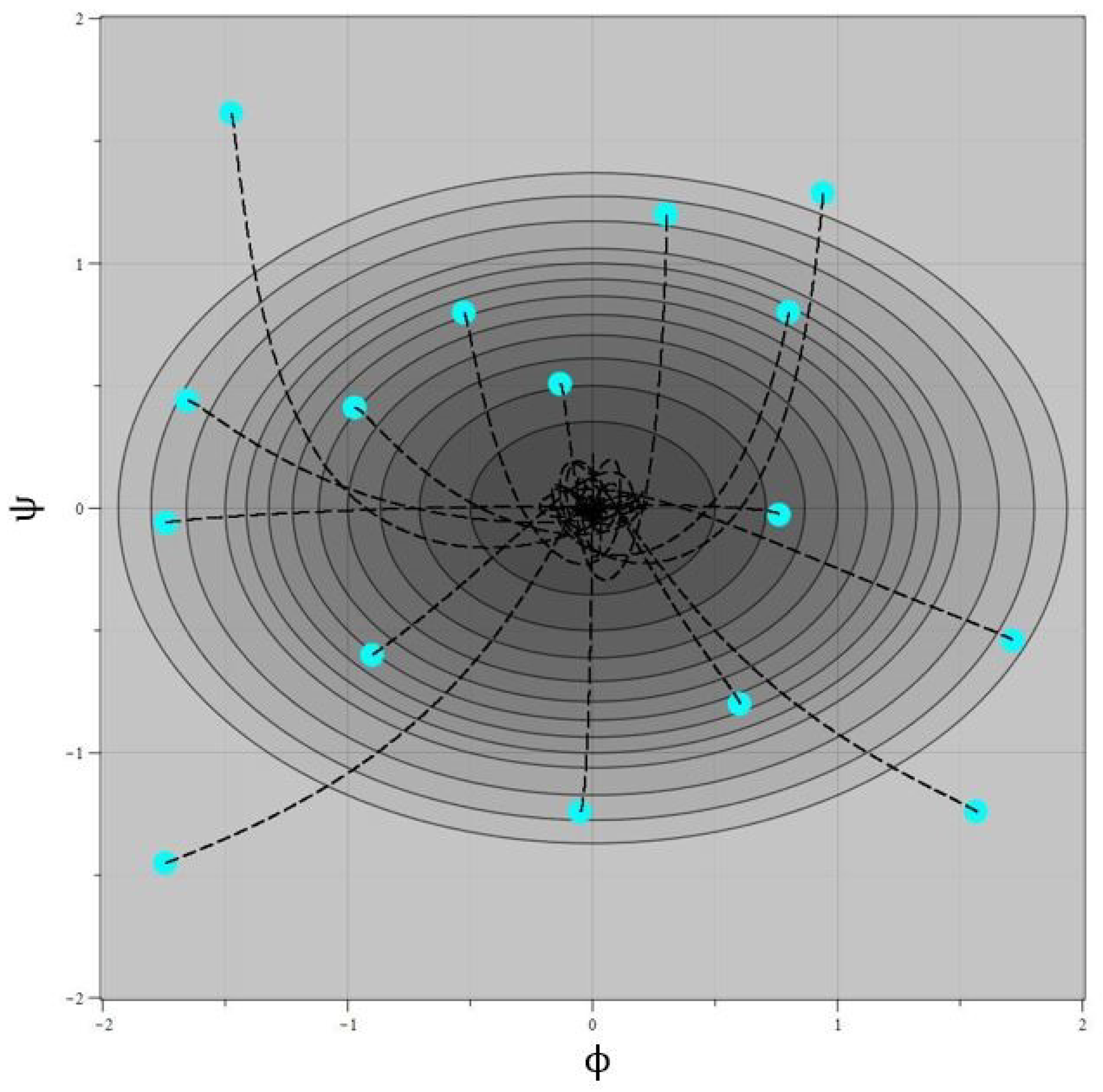
8. Example of Symmetry Braking
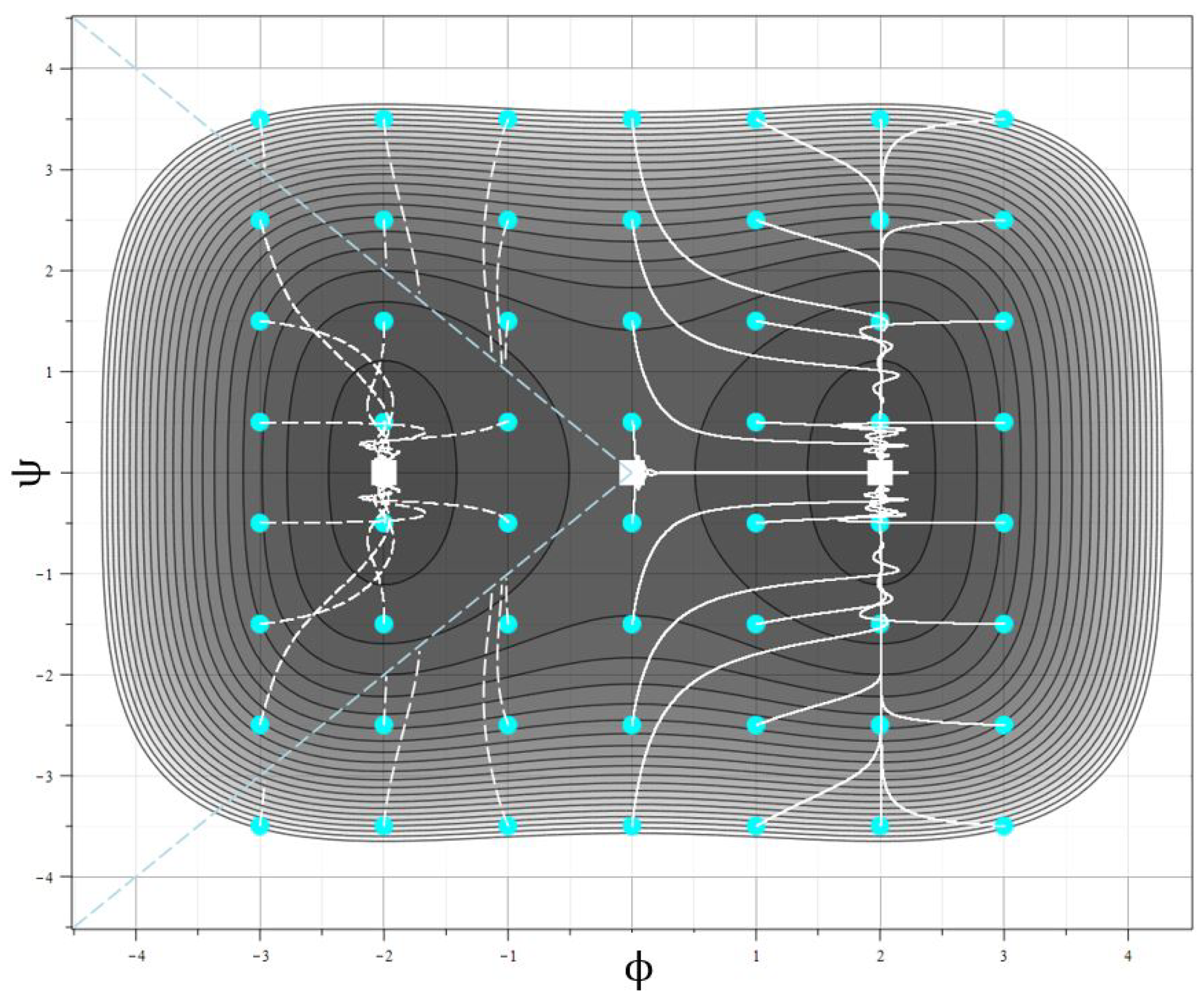
One of the most significant consequences of the appearance of special critical points in cosmological models with chiral fields is the possibility of breaking the symmetry of the potential with respect to the “rolling” of the model fields into symmetric main critical points. A simple example of such model is a model with a symmetric potential of the theory of the following form:
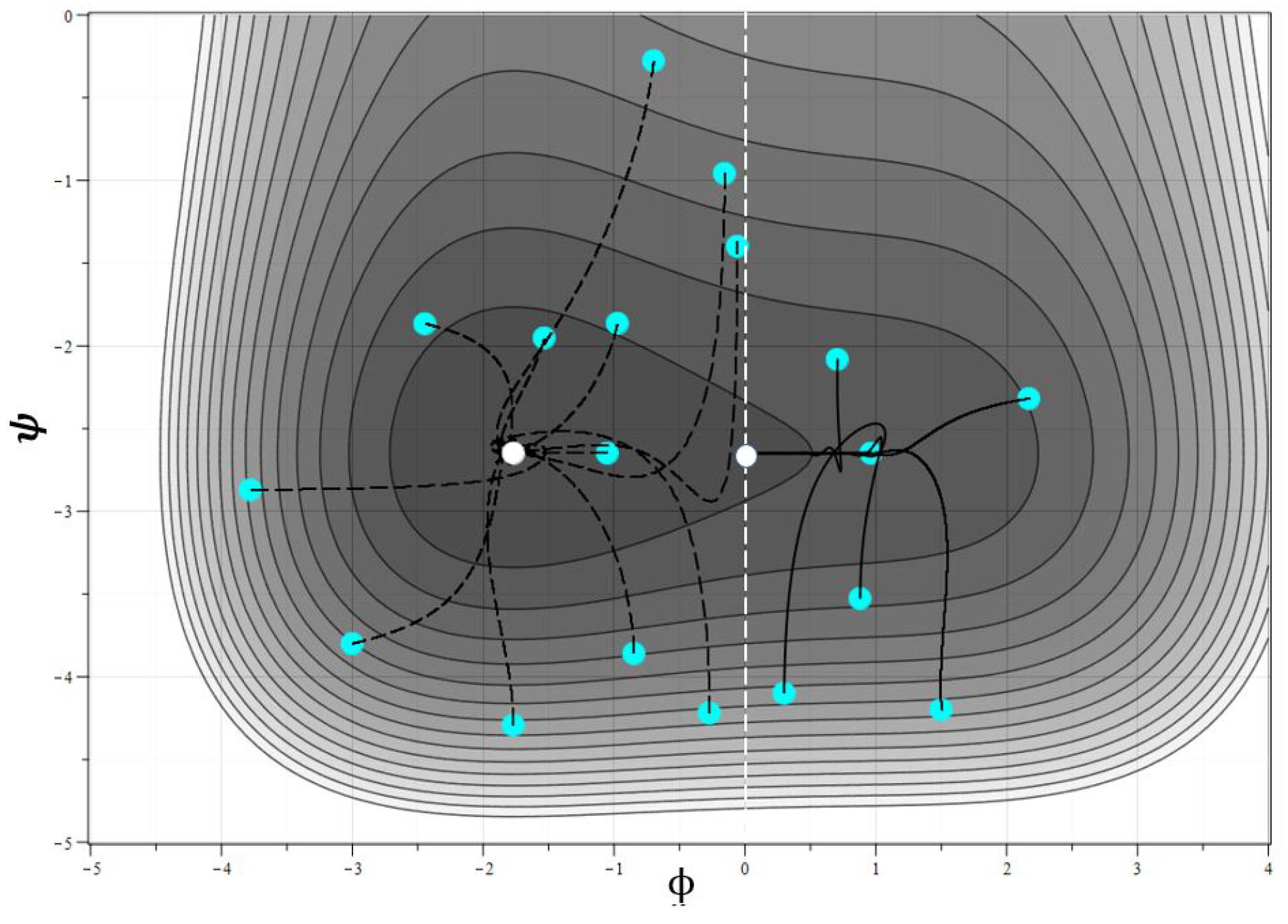
This potential has two symmetric minima at the points and one maximum at the point . These three extremes represent three major critical points for the model. The points are attracting, and is repulsive. The points are located symmetrically with respect to , which leads to the same probability of rolling the fields of the system to one of the points under random perturbations of the fields near zero, provided that has no zeros.
Let us now study the model with in the following functional form:
For such a model, the zeros of form two half-lines going out from the point . These half-lines form a barrier to which the fields roll as they tend to the main singular point . In the region where the point is located, the phase trajectories converge to this point without any obstacles.
Concerning Figure 10, (12) presents the results of a numerical analysis of the model with potential (50) and metric component (51). The phase trajectories in the projection on the isolines of the interaction potential are shown in Figure 10 for a set of 56 starting points, indicated by circles in the figure. The main feature points are indicated by squares.
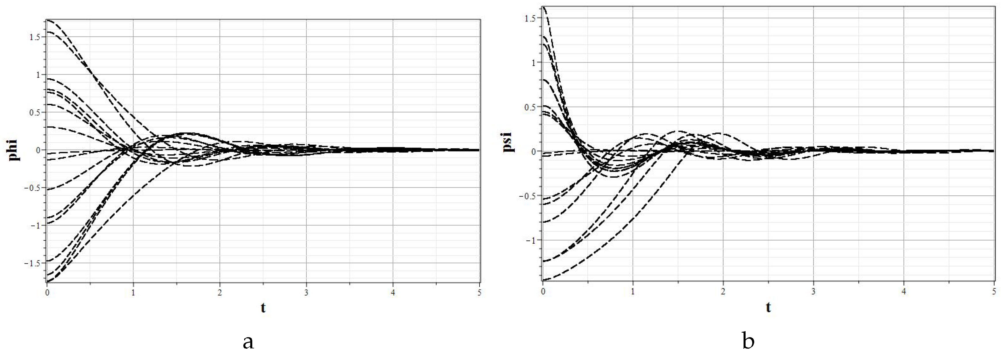
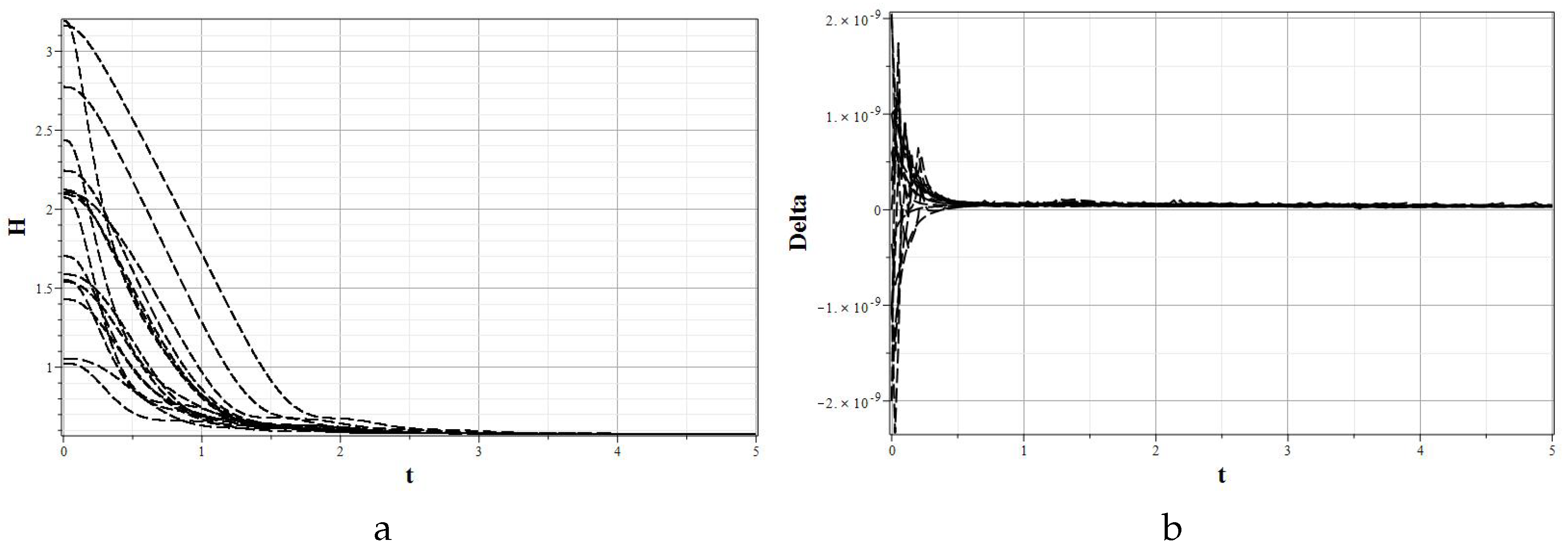
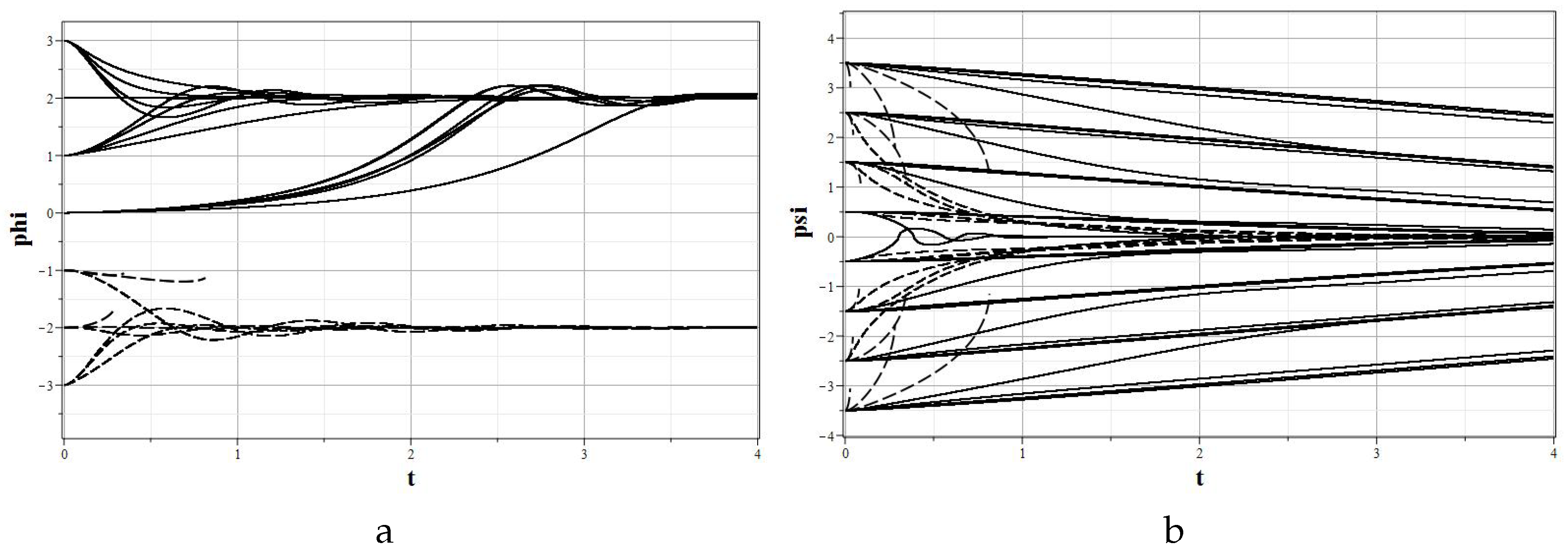
In Figure 11 graphs of field evolution with time are presented. In Figure 12 graphs of the evolution of the Hubble parameter and deviations of the integral of motion from zero are presented as well.
According to the general ideology developed above, in the region where the point is located, the phase trajectories must converge either to the main point , or to the conditional minimum of the potential on the half-straight zeros . However, the numerical model demonstrates only that the phase trajectories reach zero half-lines . Near the zeros, the numerical calculation is cut off due to peculiarities of the coefficients of the equations in these zeros. Therefore it is required additional analytical analysis of models of this type near distributed special points. Such analysis is beyond the scope of this work.
The general conclusion that can be drawn from the given example is that zeros of the metric components can break the symmetry of the models, which is only due to the symmetry of the self-action potential. This means that if only the energy of the fields is taken into account in the analysis of cosmological evolution, then the violation of symmetry such as baryon asymmetry may look like an inexplicable phenomenon. The presence of completely different mechanism associated with the zeros of the metric coefficients of the model can provide a real explanation for the violation of symmetry in one form or another.
9. Conclusions
The most important conclusion that can be drawn from the performed numerical analysis of the model are that the asymptotic behavior of chiral cosmological models is determined not only by the minima of the interaction potential.
From the analysis of the dynamics of models in which the metric component of the chiral space vanishes at some points, it follows that the presence of these zeros can significantly change the nature of cosmological evolution both with respect to the evolution of fields and with respect to the Hubble parameter. An important circumstance in this case is that the appearance of special critical points is determined by completely different physical mechanism than energy properties of the fields participating in the formation of cosmological dynamics. The properties of the chiral space are not directly related to the interaction potential of the fields. However, zeros of the metric components of these fields form completely new asymptotic behavior of the fields and the Hubble parameter. As already noted, the general behavior of the dynamics can be formally correlated with the rolling of a ball into a well in the presence of impenetrable barriers in the wall. The type of special critical point considered in this work does not fit, as noted, in the standard definitions of center, focus, saddle. The example with distributed zeros shows a rather complex change in the dynamics of the model, not related to the interaction potential. The presence of special critical points in chiral cosmological models may turn out to be an important element of cosmological dynamics with matter in the form of interacting scalar fields and requires more detailed study.
The presence of two types of critical points of the model, main and special, leads to more complex analysis of the dynamics in their vicinity using the first order perturbation theory. In this section, based on perturbation theory, complete classification of the main critical points of 2-CCM is carried out. The perturbation theory near special singular points turned out to be much more diverse than the main ones, which require separate work. Therefore, here, perturbation theory is applied only for one type of special point associated with the point zeros of the metric components of the chiral space.
Author Contributions
All of the authors contributed equally to this work. All authors have read and agreed to the published version of the manuscript.
Funding
This research was partly funded by RUSSIAN FOUNDATION OF BASIC RESEARCH grant number 20-02-00280.
Acknowledgments
S.V. C was supported by the Program of Competitive Growth of Kazan Federal University. V.M. Zh. was supported within the project 0777-2020-0018 financed from the state assignment means given to winners of the competition of scientific laboratories of educational organizations of higher education under the authority of the Ministry of Education and Science of Russia.
Conflicts of Interest
The authors declare no conflict of interest.
References
- Chervon, S.V. Chiral Cosmological Models: Dark Sector Fields Description. Quantum Matter 2013, 2, 71–82. [Google Scholar]
- Perelomov, A.M. Chiral models: Geometrical aspects. Phys. Rep. 1987, 146, 136. [Google Scholar] [CrossRef]
- Chervon, S.V.; Fomin, I.V.; Pozdeeva, E.O.; Sami, M.; Vernov, S.Y. Superpotential method for chiral cosmological models connected with modified gravity. Phys. Rev. D 2019, 100, 063522. [Google Scholar] [CrossRef] [Green Version]
- Paliathanasis, A.; Leon, G. Asymptotic behavior of N-fields Chiral Cosmology. Eur. Phys. J. C 2020, 80, 847. [Google Scholar] [CrossRef]
- Chervon, S.V.; Maharaj, S.D.; Beesham, A.; Kubasov, A.S. Emergent Universe Supported by Chiral Cosmological Fields in 5D Einstein-Gauss-Bonnet Gravity. Gravit. Cosmol. 2014, 20, 176–181. [Google Scholar] [CrossRef] [Green Version]
- Beesham, A.; Chervon, S.V.; Maharaj, S.D.; Kubasov, A.S. Exact Inflationary Solutions Inspired by the Emergent Universe Scenario. Int. J. Theor. Phys. 2015, 54, 884–895. [Google Scholar] [CrossRef]
- Chervon, S.V.; Fomin, I.V.; Beesham, A. The method of generating functions in exact scalar field inflationary cosmology. Eur. Phys. J. C 2018, 78, 301. [Google Scholar] [CrossRef] [Green Version]
- Fomin, I.V.; Chervon, S.V. Exact and Approximate Solutions in the Friedmann Cosmology. Russ. Phys. J. 2017, 60, 427–440. [Google Scholar] [CrossRef]
- Chervon, S.; Fomin, I.; Yurov, V.; Yurov, A. Series on the Foundations of Natural Science and Technology: Scalar Field Cosmology; World Scientific Publishing: Singapore, 2019; Volume 13. [Google Scholar]
- Abbyazov, R.R.; Chervon, S.V. Unified Dark Matter and Dark Energy Description in a Chiral Cosmological Model. Mod. Phys. Lett. A 2013, 28, 1350024. [Google Scholar] [CrossRef] [Green Version]
- Fijii, Y.; Maeda, K.-I. The Scalar–Tensor Theory of Gravitation; Cambridge University Press: Cambridge, UK, 2003. [Google Scholar]
- Kaiser, D.I. Conformal Transformations with Multiple Scalar Fields. Phys. Rev. D 2010, 81, 084044. [Google Scholar] [CrossRef] [Green Version]
- Kaiser, D.I.; Sfakianakis, E.I. Multifield Inflation after Planck: The Case for Nonminimal Couplings. Phys. Rev. Lett. 2014, 112, 011302. [Google Scholar] [CrossRef]
- Schutz, K.; Sfakianakis, E.I.; Kaiser, D.I. Multifield Inflation after Planck: Isocurvature Modes from Nonminimal Couplings. Phys. Rev. D 2014, 89, 064044. [Google Scholar] [CrossRef] [Green Version]
- Aghanim, N.; Akrami, Y.; Ashdown, M.; Aumont, J.; Baccigalupi, C.; Ballardini, M.; Banday, A.J.; Barreiro, R.B.; Bartolo, N.; Basak, S.; et al. [Planck Collaboration], Planck 2018 results. VI. Cosmological parameters. arXiv 2018, arXiv:1807.06209. [Google Scholar]
- Akrami, Y.; Arroja, F.; Ashdown, M.; Aumont, J.; Baccigalupi, C.; Ballardini, M.; Banday, A.J.; Barreiro, R.B.; Bartolo, N.; Basak, S.; et al. [Planck Collaboration], Planck 2018 results. X. Constraints on inflation. arXiv 2018, arXiv:1807.06211. [Google Scholar]
- Gong, J.O. Multi-field inflation and cosmological perturbations. Int. J. Mod. Phys. D 2016, 26, 1740003. [Google Scholar] [CrossRef]
- Kallosh, R.; Linde, A. Multi-field Conformal Cosmological Attractors. J. Cosmol. Astropart. Phys. 2013, 2013, 006. [Google Scholar] [CrossRef] [Green Version]
- Abbyazov, R.R.; Chervon, S.V.; Müller, V. σCDM coupled to radiation: Dark energy and Universe acceleration. Mod. Phys. Lett. A 2015, 30, 1550114. [Google Scholar] [CrossRef] [Green Version]
- Abbyazov, R.R.; Chervon, S.V. Interaction of chiral fields of the dark sector with cold dark matter. Gravit. Cosmol. 2012, 18, 262–269. [Google Scholar] [CrossRef]
- Naruko, A.; Yoshida, D.; Mukohyama, S. Gravitational scalar-tensor theory. Class. Quant. Grav. 2016, 33, 09LT01. [Google Scholar] [CrossRef] [Green Version]
- Chervon, S.V.; Fomin, I.V.; Mayorova, T.I. Chiral cosmological model of f(R) gravity with a kinetic curvature scalar. Gravit. Cosmol. 2019, 25, 205–212. [Google Scholar] [CrossRef]
- Chervon, S.V.; Nikolaev, A.V.; Mayorova, T.I. On the derivation of field equation of f(R) gravity with kinetic scalar curvature. Spacetime Fundam. Interact. 2017, 1, 30–37. [Google Scholar] [CrossRef]
- Chervon, S.V.; Nikolaev, A.V.; Mayorova, T.I.; Odintsov, S.D.; Oikonomou, V.K. Kinetic scalar curvature extended f(R) gravity. Nucl. Phys. 2018, B936, 597–614. [Google Scholar] [CrossRef]
- Saridakis, E.N.; Tsoukalas, M. Cosmology in new gravitational scalar-tensor theories. Phys. Rev. D 2016, 93, 124032. [Google Scholar] [CrossRef] [Green Version]
- Chervon, S.V.; Fomin, I.V.; Mayorova, T.I.; Khapaeva, A.V. Cosmological parameters of f(R) gravity with kinetic scalar curvature. J. Phys. Conf. Ser. 2020, 1557, 012016. [Google Scholar] [CrossRef]
- Bogoyavlensky, O.I. Methods of the Qualitative Theory of Dynamical Systems in Astrophysics and Gas Dynamics; Publishing Nauka: Moscow, Russia, 1980. [Google Scholar]
- Starobinsky, A.A. A New Type of Isotropic Cosmological Models Without Singularity. Phys. Lett. B 1980, 91, 99–102. [Google Scholar] [CrossRef]
- Starobinsky, A.A. Dynamics of phase transition in the new inflationary universe scenario and generation of perturbations. Phys. Lett. B 1982, 117, 175–178. [Google Scholar] [CrossRef]
- Belinsky, V.A.; Grishchuk, L.P.; Khalatnikov, I.M.; Zeldovich, Y.B. Inflationary stages in cosmological models with a scalar field. Phys. Lett. B 1985, 155, 232–236. [Google Scholar] [CrossRef]
- Coley, A.A. Dynamical Systems and Cosmology; Springer-Science+Business Media: Dordrecht, The Netherlands, 2003. [Google Scholar]
- Coley, A.A. Proceedings of the Sixth Canadian Conference on General Relativity and Relativistic Astrophysics; Braham, S., Gegenberg, J., McKellar, R., Eds.; Fields Institute Communications Series (AMS): Providence, RI, USA, 1997; p. 19. [Google Scholar]
- Wainwright, J.; Ellis, G.F.R. Dynamical Systems in Cosmology; Cambridge University Press: Cambridge, UK, 1997. [Google Scholar]
- Copeland, E.J.; Sami, M.; Tsujikawa, S.J. Dynamics of dark energy. Int. J. Mod. Phys. D 2006, 15, 1753–1936. [Google Scholar] [CrossRef] [Green Version]
- Ignat’ev, Y.G.; Agathonov, A.A. Qualitative and numerical analysis of a cosmological model based on a phantom scalar field with self-interaction. Grav.Cosmol. 2017, 23, 230–235. [Google Scholar] [CrossRef]
- Ignat’ev, Y.G.; Agathonov, A.A. Qualitative and Numerical Analysis of the Cosmological Model Based on a Phantom Scalar field with Self-Action. II. Comparative Analysis of Models of Classical and Phantom Fields. arXiv 2017, arXiv:1706.05619. [Google Scholar]
- Ignat’ev, Y.G.; Kokh, I.A. Qualitative and Numerical Analysis of a Cosmological Model Based on an Asymmetric Scalar Doublet with Minimal connections. IV. Numerical Modeling and Types of Behavior of the Model. Russ. Phys. J. 2019, 3, 453–470. [Google Scholar] [CrossRef] [Green Version]
- Zhuravlev, V.M. Qualitative analisys of cosmological models with scalar fields. Spacetime Fundam. Interact. 2016, 4, 39–51. [Google Scholar] [CrossRef]
- Ignat’ev, Y.G.; Agathonov, A.A. The Peculiarities of the Cosmological Models Based on Non-Linear Classical and Phantom Fields with Minimal Interaction. I. The Cosmological Model Based on Scalar Singlet. arXiv 2018, arXiv:1808.04570. [Google Scholar]
- Ignat’ev, Y.G.; Agathonov, A.A. The Peculiarities of the Cosmological Models Based on Nonlinear Classical and Phantom Fields with Minimal Interaction. II. The Cosmological Model Based on the Asymmetrical Scalar Doublet. arXiv 2018, arXiv:1810.09873. [Google Scholar]
- Zhuravlev, V.M.; Podymova, T.V.; Pereskokov, E.A. Cosmological Models with a Specified Trajectory on the Energy Phase Plane. Gravit. Cosmol. 2011, 17, 101–109. [Google Scholar] [CrossRef]
- Ignat’ev, Y.G. Standard cosmological model: Mathematical, qualitatively and numerical analysis. Spacetime Fundam. Interact. 2016, 3, 17–36. [Google Scholar] [CrossRef]
- Chervon, S.V. On the chiral model of cosmological inflation. Russ. Phys. J. 1995, 38, 539. [Google Scholar] [CrossRef]
- Chervon, S.V. Chiral non-linear sigma models and cosmological inflation. Gravit. Cosmol. 1995, 1, 91. [Google Scholar]
- Chervon, S.V.; Fomin, I.V.; Kubasov, A.S. Scalar and Chiral Fields in Cosmology; Ulyanovsk State Pedagogical University: Ulyanovsk, Russia, 2015. (In Russian) [Google Scholar]
Figure 1.
Isolines of the interaction potential (45) with phase trajectories for a set of 16 starting points.
Figure 1.
Isolines of the interaction potential (45) with phase trajectories for a set of 16 starting points.

Figure 2.
Dependence of the fields (a) and (b) on t for the potential (45).
Figure 2.
Dependence of the fields (a) and (b) on t for the potential (45).

Figure 3.
Dependence of H on t (a); deviation of the integral of motion from zero (b).

Figure 4.
Isolines of the interaction potential (47) together with the phase trajectories of the model.
Figure 4.
Isolines of the interaction potential (47) together with the phase trajectories of the model.

Figure 5.
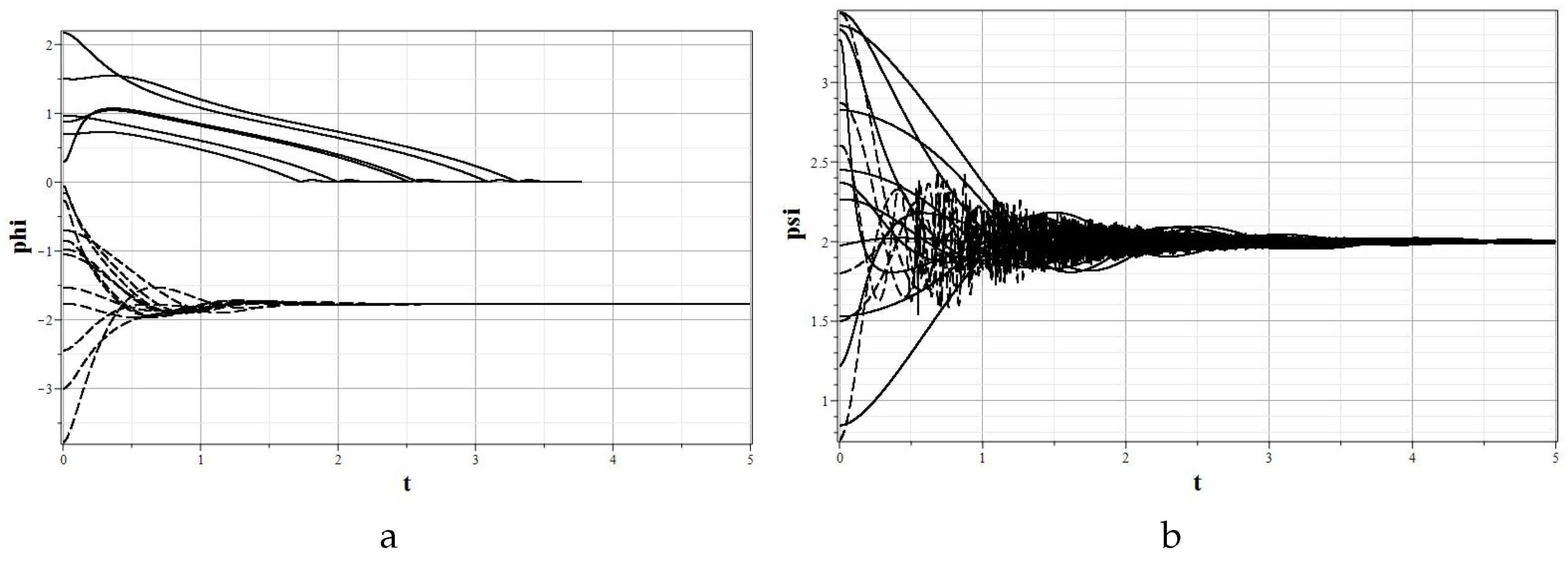
Dependence of the fields (a) and (b) on t for the potential (47).
Figure 5.
Dependence of the fields (a) and (b) on t for the potential (47).

Figure 6.
Dependence of H on t (a); deviation of the integral of motion from zero (b).

Figure 7.
Isolines of the interaction potential (47) together with the phase trajectories of the model.
Figure 7.
Isolines of the interaction potential (47) together with the phase trajectories of the model.

Figure 8.
Dependence on t of the fields (a) and (b).

Figure 9.
Dependence of H on t (a); deviation of the integral of motion from zero (b).


Figure 11.
Changing fields over time: (a) , (b) .

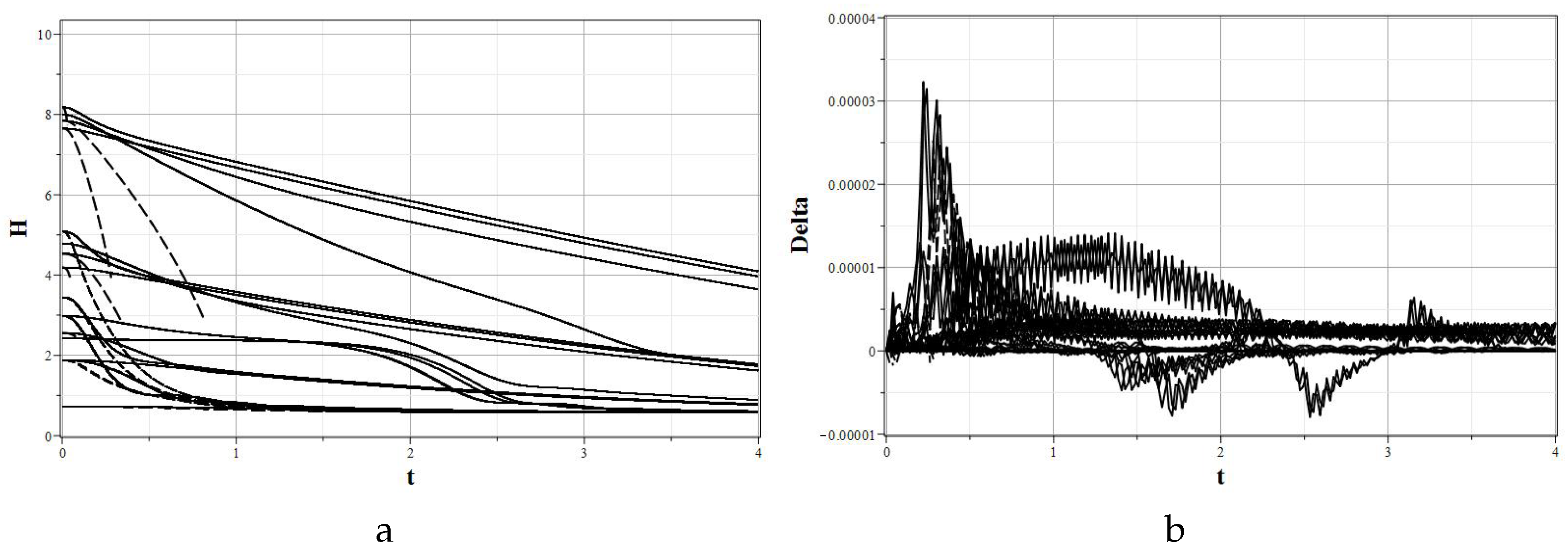
Figure 12.
Dependence of H on t (a); deviation of the integral of motion from zero (b).

Publisher’s Note: MDPI stays neutral with regard to jurisdictional claims in published maps and institutional affiliations. |
© 2020 by the authors. Licensee MDPI, Basel, Switzerland. This article is an open access article distributed under the terms and conditions of the Creative Commons Attribution (CC BY) license (http://creativecommons.org/licenses/by/4.0/).
Share and Cite
MDPI and ACS Style
Zhuravlev, V.; Chervon, S. Qualitative Analysis of the Dynamics of a Two-Component Chiral Cosmological Model. Universe 2020, 6, 195. https://0-doi-org.brum.beds.ac.uk/10.3390/universe6110195
AMA Style
Zhuravlev V, Chervon S. Qualitative Analysis of the Dynamics of a Two-Component Chiral Cosmological Model. Universe. 2020; 6(11):195. https://0-doi-org.brum.beds.ac.uk/10.3390/universe6110195
Chicago/Turabian StyleZhuravlev, Viktor, and Sergey Chervon. 2020. "Qualitative Analysis of the Dynamics of a Two-Component Chiral Cosmological Model" Universe 6, no. 11: 195. https://0-doi-org.brum.beds.ac.uk/10.3390/universe6110195
Note that from the first issue of 2016, this journal uses article numbers instead of page numbers. See further details here.